The Odds Exponential-Pareto IV Distribution: Regression Model and Application


1
Department of Statistics, Faculty of Science, King Abdulaziz University, Jeddah 21589, Saudi Arabia
2
Department of Statistics, Faculty Science, University of Jeddah, Jeddah 21959, Saudi Arabia
*
Author to whom correspondence should be addressed.
Entropy 2020, 22(5), 497; https://doi.org/10.3390/e22050497
Submission received: 19 March 2020
/
Revised: 15 April 2020
/
Accepted: 23 April 2020
/
Published: 25 April 2020
(This article belongs to the Section Information Theory, Probability and Statistics)
Abstract
:This article introduces the odds exponential-Pareto IV distribution, which belongs to the odds family of distributions. We studied the statistical properties of this new distribution. The odds exponential-Pareto IV distribution provided decreasing, increasing, and upside-down hazard functions. We employed the maximum likelihood method to estimate the distribution parameters. The estimators performance was assessed by conducting simulation studies. A new log location-scale regression model based on the odds exponential-Pareto IV distribution was also introduced. Parameter estimates of the proposed model were obtained using both maximum likelihood and jackknife methods for right-censored data. Real data sets were analyzed under the odds exponential-Pareto IV distribution and log odds exponential-Pareto IV regression model to show their flexibility and potentiality.
1. Introduction
Pareto distribution was named after the Italian economist Vilfredo Pareto (1848–1923). The Pareto distribution has gained considerable attention in modeling many applications with heavy-tailed distributions, such as income distribution, earthquakes, forest fire areas, and disk drive sector errors [1,2]. The Pareto IV family is a general family of distributions. Pareto I, Pareto II, and Pareto III distributions are special cases of the Pareto IV family. Also, the Burr family can be regarded as a special case of Pareto IV (see, [3,4]). There are several studies in the literature generalizing the Pareto distribution to make it richer and more flexible for modeling data. These include the generalized Pareto [5], beta-Pareto [6], beta-generalized Pareto [7], Weibull–Pareto [8], gamma-Pareto [9,10], Kumaraswamy exponentiated Pareto [11], and exponentiated Weibull–Pareto distribution [12].
In recent works, adding new parameters to existing distributions or using different methods makes the resulting new distribution more appropriate and efficient for modeling the lifetime data. Many distributions have been generalized in the literature. These include the logit of the Kumaraswamy distribution [13], the generalized beta-generated distribution [14], the Weibull-G family of distribution [15], the gamma-exponentiated exponential distribution [16], and the transmuted Weibull-Pareto distribution [17]. Very recently, some new odd distributions were proposed in the literature, such as the odd Birnbaum–Saunders distribution [18], the odd Burr-III family of distributions [19], the odds exponential-log logistic distribution [20], the odd log-logistic-Fréchet distribution [21], the odd log-logistic-Burr XII distribution [22], the odd exponentiated half-logistic Burr XII distribution [23], the odd Lomax-G family of distributions [24], the odd Dagum-G family of distributions [25], and the odd log-logistic Lindley-exponential distribution [26].
This article used the transformed-transformer (T-X) family by Alzaatreh et al. [27] to introduce an odds exponential-Pareto IV distribution, in which the cumulative distribution function (CDF) is defined by
where r(t) is the probability density function (PDF) of a random variable , such that and W(F(x)) is a function of any CDF, that takes different forms, see Alzaatreh et al. [27]. In this study, we consider the odds function form, . That is, the CDF will be
and we considered the exponential distribution for and is the Pareto IV distribution with parameters in Equation (2). The resulting generated distribution will provide more flexibility in accommodating different types of the hazard function for the generated distribution. Also, this proposed distribution will be more suitable for modeling and fitting different real-life data
Therefore, we now define the odds exponential-Pareto IV (OEPIV) distribution with CDF given by
The PDF of OEPIV is
where , are the shape parameters, is the scale parameter, and is the inequality parameter.
Recently, there has been a great deal of interest in the literature investigating the relationship between survival time and some other covariates, such as sex, weight, blood pressure, and many others. In a number of applications, different parametric regression models were used to estimate the effect of covariate variables on the survival time, including the log-location-scale regression model. The log-location-scale regression model is distinguished since it is commonly used in clinical trials and in many other fields of application. It is also widely used in engineering models where failure is accelerated by voltage, temperature, or other stress factors [28]. Several studies in the literature applied the log-location-scale regression model based on different distributions, such as the log-modified Weibull [29], the log-Weibull extended [30], the log-exponentiated Weibull [31], the log-Burr XII [32], the log-beta Weibull [33], the log-beta log-logistic [34], the log-Fréchet [35], the log-Exponentiated Fréchet [36], and the log-gamma-logistic [37]. Recent studies used the log-location-scale regression model built from the logarithm odd of the distribution. For instance, the odd log-logistic-Weibull [38], odd log-logistic generalized half normal [39], and odd Weibull [40].
This article is organized as follows: In Section 2, we define the survival and hazard functions of the OEPIV distribution with some graphical representations. We derived some of the OEPIV properties in Section 3. In Section 4, we explain the maximum likelihood estimation for parameters of the odds exponential-Pareto IV distribution. Simulation studies are provided to illustrate the performance of the OEPIV distribution in Section 5. In Section 6, we address the log odds exponential-Pareto IV (LOEPIV) distribution along with some of its statistical properties, in addition to introducing a log-location regression model based on LOEPIV and discussed its parameter estimates via maximum likelihood and Jackknife methods. In Section 7, three applications are analyzed to demonstrate the performance of the introduced new distribution and its regression model. Finally, we report our conclusions in Section 8.
2. The Odds Exponential-Pareto IV Distribution
The survival (SF) and hazard functions (HF) are, respectively, as follows:
The Exponential-Pareto (EP) distribution [41] can be treated as a special case of OEPIV distribution by setting and . For , and , we obtain the odds exponential-log logistic (OELL) distribution [20].
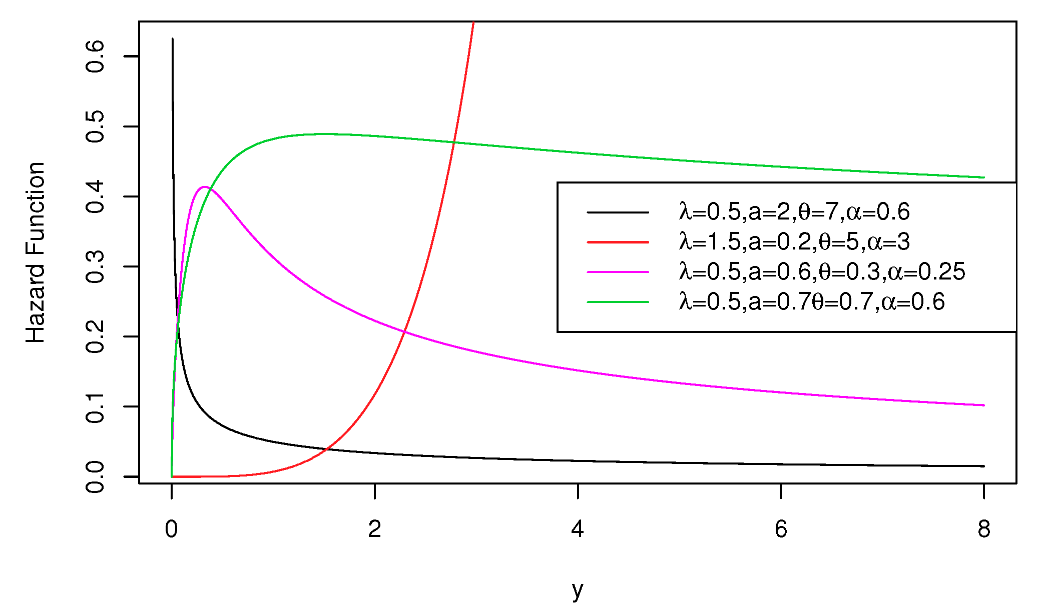
Graphical representations of the PDF in Equation (4) and HF in Equation (6) are, respectively, shown in Figure 1 and Figure 2. From Figure 1, we note that the OEPIV distribution has different shapes at different parameter values, which indicate its great flexibility. Based on Figure 2, the OEPIV takes the following HF shapes: increasing, decreasing, and upside-down.
3. Statistical Properties
We discuss in this section some statistical properties of the OEPIV distribution.
3.1. The Quantile and Median
The quantile of the OEPIV distribution is computed as
Then, the median of the OEPIV distribution can be obtained by setting in Equation (7),
3.2. The Mode
The mode of the OEPIV distribution can be obtained by computing the derivative of the log PDF in Equation (4) with respect to x and equating to zero
Thus, the mode can be obtained numerically by solving Equation (9).
3.3. The r-th Order Moment and Moment Generating Function
The r-th order raw moment is defined as
Thus,
Let
Also,
Thus, we put the above formulas in the integration to have
Using the binomial expansion of , we obtain
Using the gamma function definition,
Thus, the r-th moment can be written as
Therefore, the moment generating function (mgf) can be obtained based on r-th moment of OEPIV distribution as
Then, the mean of the OEPIV distribution is
The mean, variance, skewness, and kurtosis of the OEPIV distribution for different values of , a, , and are calculated in Table 1, to illustrate the effects on these measures.
3.4. Order Statistics
Suppose is a random sample from the PDF in Equation (4). Let , denote the corresponding order statistic. The probability density function and the cumulative distribution function of the order statistic, say , given by
where and are the PDF and CDF of OEPIV distribution given by Equations (4) and (3), respectively. Using the binomial expansion of , given as follows
Using binomial expansion of , we get
3.5. Rényi Entropy
The Rényi entropy of a random variable X represents a measure of variation of the uncertainty. It is given by
Let , so
Using binomial expansion of , given as follows
Thus, we put the above formula in the integration to have
The Rényi entropy of the OEPIV distribution is
4. Estimation of the OEPIV Parameters
We assume that is a random sample from the OEPIV distribution. Then, the log-likelihood (ℓ) for is
where . The likelihood equations are given by
and
We can obtain maximum likelihood (ML) estimates of the parameters by directly maximizing Equation (17) using the nlm or optim functions in R package or by solving Equations (18)–(21). Under standard regularity conditions, we can obtain approximate intervals estimation of the parameters using multivariate normal distribution by numerically evaluating the elements of the observed information matrix at , . In addition, the likelihood ratio (LR) test can be applied to discriminate between nested models.
5. Simulation Studies
We conducted a Monte Carlo simulation to illustrate the performance of the ML parameter estimates of the OEPIV distribution. That is, we randomly generated 10,000 samples with size 30, 50, 100, 200, and 500 from the OEPIV distribution for two different sets of parameter values as follows:
The estimates for the parameters were obtained along with their calculated bias and mean square error (MSE), given by
where . The results of the simulation are displayed in Table 2. We concluded from these results that the empirical means tend to the true value of the parameters as the sample size increases. In addition, the MSEs and biases decreased as we increased the sample size.
6. The Log Odds Exponential-Pareto IV Regression Model
If X is a random variable from the OEPIV distribution, as given in Equation (4), then is a random variable that has a LOEPIV distribution with the transformation parameter and . Therefore, the PDF and CDF of the LOEPIV distribution are as follows:
where is the scale parameter, , are the shape parameters, and is the location parameter. The LOEPIV model becomes the log exponential-Pareto (LEP) distribution for . The PDF (for ) of the LEP distribution with parameters , and , is
The SF and HF are given by
The following are the properties for the LOEPIV distribution:
The quantile of the LOEPIV distribution
The mode of the LOEPIV distribution
Then, the mode can be obtained by solving Equation (27) numerically.
The median of the LOEPIV distribution
The mgf of LOEPIV distribution
Thus,
Substituting will reduce the above integration to
Then, using the binomial expansion
can be rewritten as
Using the gamma function. Thus, the mgf of LOEPIV distribution is as follows
The standardized random variable for y in Equation (22) is defined as , then z has the following PDF
with SF given as
Hence, a linear location-scale regression model with response variable and explanatory vector can be defined as
where is the random error with PDF in Equation (24), , and , , and are the unknown parameters. is the location of and the location vector can be represented as a linear model , in which is the known model matrix. Therefore, the SF of is expressed as:
6.1. Estimation of the LOEPIV Regression Model
6.1.1. ML Method
For the right-censored lifetime data, we have , where is the lifetime and is the censoring time, then, we have for the individual . If we have a random sample with n observations ,...,, where , and assuming the censoring and lifetimes are independent and random. Then, the likelihood function for the regression model in (31) with assuming right censoring is as follows:
where and are given by Equations (17) and (19) of , respectively. The ℓ for reduces to
where represents the uncensored data, and . The ML estimate for the parameter vector could be obtained using an optimization algorithm that maximizes Equation (32).
6.1.2. Jackknife Method
The jackknife technique was developed by Quenouille (1949) to estimate the bias of an estimator. It is an alternative method to estimate the LOEPIV parameters based on “leaving one out”.
Suppose that is the parameter estimation of the whole sample and is the parameter estimation when we dropped the observation from the data. That is, the pseudo-value of the observation is obtained as
Then, the jackknife estimate of is the mean of pseudo-values, denoted is
6.2. Sensitivity Analysis: Global Influence
Global influence, introduced by [45], is used to conduct a sensitivity analysis that represents the diagnostic effect depending on the case deletion. Case deletion measures the impact of dropping the observation from the data set on the estimate of the parameters. That is, this method is based on comparing the difference of and where is the estimated parameters when the observation is dropped from data. If is distant from , then this case is considered as influential. The case deletion model for the LOEPIV regression Model (31) is
We denote the ML estimate of when the observation is dropped by . Then, we describe two methods of global influence below.
6.2.1. Generalized Cook Distance
Generalized Cook distance (GD) is the first measure of global influence and is defined as
where denotes the observed information matrix.
6.2.2. Likelihood Distance
Likelihood distance (LD) measures the differences between and , and is given by
where is the log likelihood function of when the observation is dropped from the data.
6.3. Residual Analysis
In the regression model, checking the assumptions and appropriateness of the fitted model is an essential step. Therefore, we used residual analysis to check the assumptions and detect outlier observations. In this study, we consider the following types.
6.3.1. Martingale Residual
Barlow and Prentice [46] proposed the martingale residual as
where denotes the censor indicator, where , if the observation is censored, and , if the observation is not censored, and denotes the SF for the regression model. Therefore, the martingale residual of the LOEPIV regression model is
where has a range between and 1 and has skewness. Thus, the transformation of will be used to reduce the skewness.
6.3.2. Deviance Residual
This is a further improvement of the martingale residual, which reduces the skewness and make it more symmetrical, around zero. It can be expressed as
where is defined in Equation (36), and the deviance for the LOEPIV regression model is
7. Simulation Study for the Log Odds Exponential-Pareto IV Regression Model
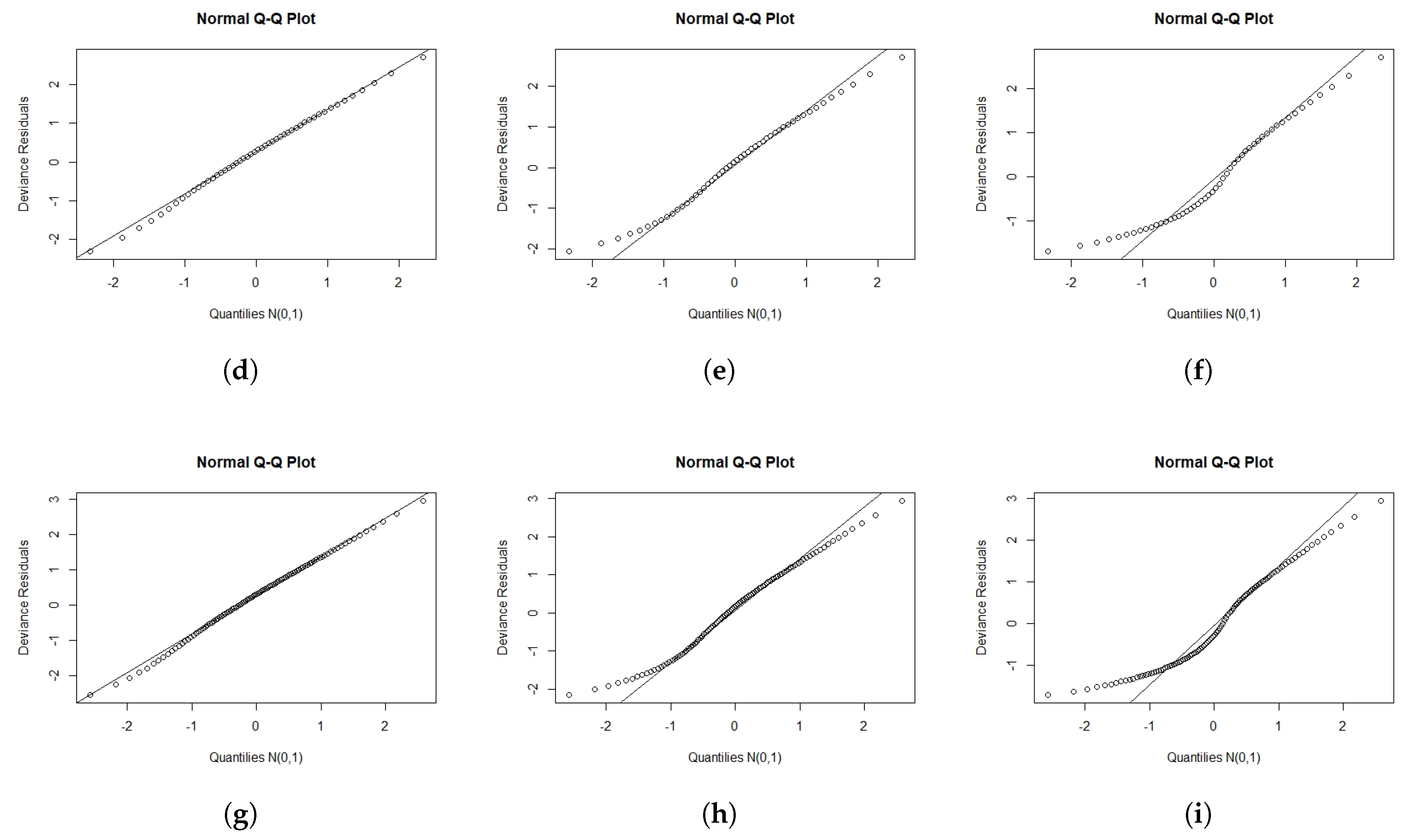
We performed a Monte Carlo simulation to explore the empirical distribution of the and for different values of n and different censoring levels. The lifetimes were from the OEPIV distribution in Equation (4), and was generated from uniform . We sampled the censoring times from uniform , where was adjusted until we obtained the required censoring level. For each fit, the log lifetimes were obtained as . We generated 1000 samples. For each selection of , and , and the censoring levels. The simulation was conducted for , 50, and 100 with , , , , and , and the censoring levels 0.1, 0.3, and 0.5. Figure 3 and Figure 4 present normal probability plots (NPP) for the residuals. These figures show that the empirical distribution provided more agreement with the standard normal distribution (SND) compared to . also approached the SND as we increased the sample size or decreased the censoring level.
8. Applications
We analyzed three real data sets to investigate the flexibility of the OEPIV distribution and the LOEPIV regression model.
8.1. The Strength of Glass Fibers Data
This data was analyzed by [47], and it represents the strength of glass fibers with the length 1.5 cm. This data consists of 63 observations.
We will compare the fits of the OEPIV with the Pareto IV, Weibull BurrXII (WBXII) in [48], Weibull Frechet (WFr) in [49], Weibull Lomax (WL) in [50], Odd exponential-weibull (OE-W), Odd exponential-normal (OE-N) in [51], and Gamma distributions.
We considered the following criteria to compare these distributions: the values of the negative log-likelihood function (), Akaike information criterion (AIC), and corrected Akaike Information Criterion (CAIC). The smaller the values for these statistics, the better the fit to the data.
The ML estimates, standard errors (SE), , AIC and CAIC statistics for the OEPIV, WBXII, WL, WFr, Pareto IV,OE-W, OE-N, and Gamma distributions are reported in Table 3. From the results in Table 3, it is clear that the OEPIV distribution provides better fit for the data having lowest AIC and CAIC values and could be selected as a more appropriate model than other models. Figure 5 displays the QQ-plot of the OEPIV distribution and the estimated PDFs of the fitted distributions. It is clear from these plots that the OEPIV captures the skewness of the glass fibers data than other competitive fitted distributions.
8.2. Sum of Skin Folds Data
The authors of [52] discussed this data set, and it represents 102 male and 100 female athletes collected at the Australian Institute of Sports, provided by Richard Telford and Ross Cunningham.
We compare the ML estimates and their corresponding SE, and the values of the (), and the AIC and CAIC statistic for fitted OEPIV distribution with the results of the Kumaraswamy Pareto-IV (KwPIV) in [53], gamma-Pareto IV (GPIV) [10], Pareto IV (PIV) in [53], and exponentiated Pareto (EP) distributions provided in [54], and the Weibull distribution. These results are reported in Table 4. From the results in Table 4, it is clear that the OEPIV distribution provides the lowest AIC and CAIC values among those of the fitted distributions. Therefore, OEPIV could be selected as the best modal for this data. Figure 6 displays the QQ-plot of the OEPIV distribution and the estimated PDFs of the fitted distributions. It is clear from these plots that the OEPIV provides a good fit to this data.
8.3. Stanford Heart Transplant Data
This data was obtained from Kalbfleisch and Prentice [55] and has information on n = 103 patients. The patient’s survival time was specified as the number of days from the acceptance into a heart transplant program to death. The following are associated with each patient: : log survival time (days); : censoring indicator (1 = dead, 0 = censoring); : is the age (in years); : is the prior surgery coded as (0 = No, 1 = Yes); and : is the transplant coded as (0 = No, 1 = Yes). This data set was used by [38], [35], and [36] for illustrating the log-odd log-logistic Weibull (LOLLW), log-Fréchet (LF), and log-exponentiated Fréchet (LEF) regression models. The LOEPIV regression model will be compared with the log-Weibull (LW), LEP, LOLLW, LF, and LEF regression models.
That is, we present the results from fitting the following model
where follows the LOEPIV distribution in Equation (22).
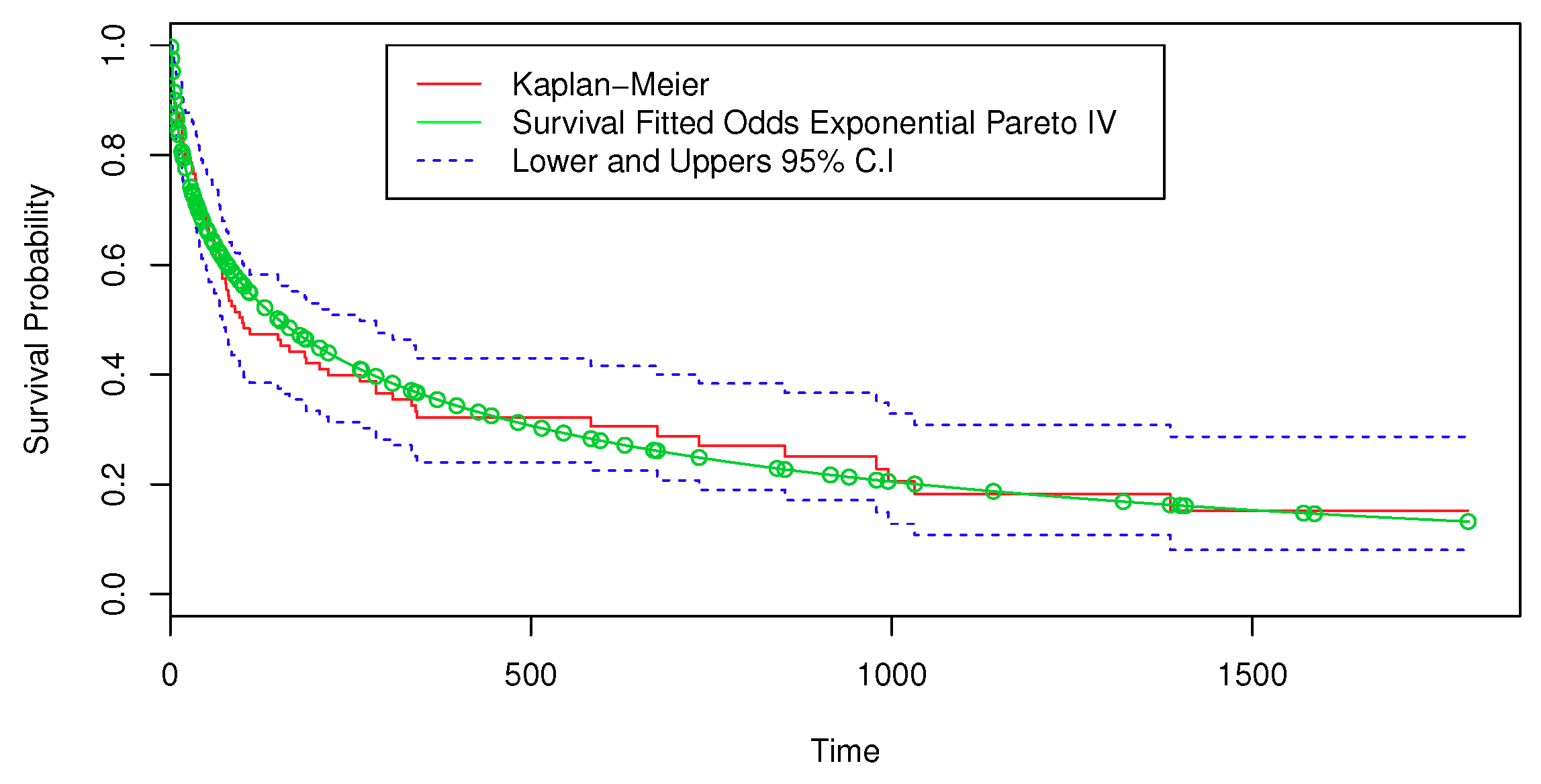
To examine the suitability of the proposed model, a plot of the empirical SF estimates from the Kaplan–Meier (KM) model and the SF from the fitted OEPIV model are displayed in Figure 7. Therefore, we concluded that the logarithm of times to event follow the LOEPIV distribution.
8.3.1. ML and Jackknife Estimation
The estimates, their corresponding SE, p-values, AIC, CAIC, and Bayesian Information Criterion (BIC) statistics for the LOEPIV, LEF, LOLLW, LF, LW and LEP regression models are shown in Table 5. The results demonstrated that the LOEPIV regression model had the lowest AIC, CAIC, and BIC. This shows the superiority of the LOEPIV model over other models. The LR test can be used to discriminate between LOEPIV and LEP regression models since they are nested.That is, the LR statistic for testing the hypotheses versus is not true given in Table 6 and rejects the LEP model in favor of the LOEPIV model.
Table 7 lists the jackknife parameter estimates of the LOEPIV model, their corresponding SE and 95% confidence intervals. Based on the results in Table 5 and Table 7, we observed that the explanatory variables , , and are significant for the fitted model and both methods displayed similar estimates.
The plots of the SF that corresponded to the explanatory variables for the fitted LOEPIV regression model are presented in Figure 8. From Figure 8a, we observed that , which means that ≈ 97% of the patients who are 8 years old will be thriving when y = 1 (≈3 days). However, for patients between 44 and 64 years old, and , which indicated that the percentages of living patients at y = 1 decreased to 34% and 0.06%, respectively. These results indicate decreases in survival of the patients as their age increased. Similarly, Figure 8b,c indicated that approximately 58% of patients who did not have surgery or receive a transplant were thriving at y = 3 (≈21 days). Furthermore, for the patients who undertook surgery, we observed that approximately 98% of them were thriving at y = 3, while patients that received a transplant, , increased to 99% at y = 3 in the survival percentage. Therefore, it can be stated that receiving a heart transplant increased the survival time when undergoing surgery.
8.3.2. Global Influence Analysis
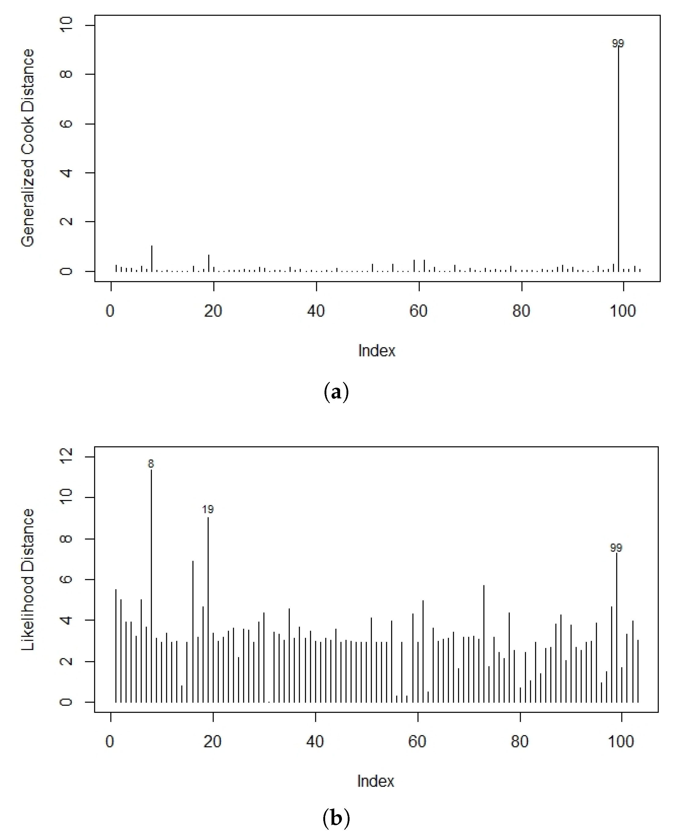
The case deletion measures and were numerically computed and Figure 9 represents the influence measure index plots. It is clear that case 99 could be an influential observation in the LOEPIV regression model.
8.3.3. Residual Analysis
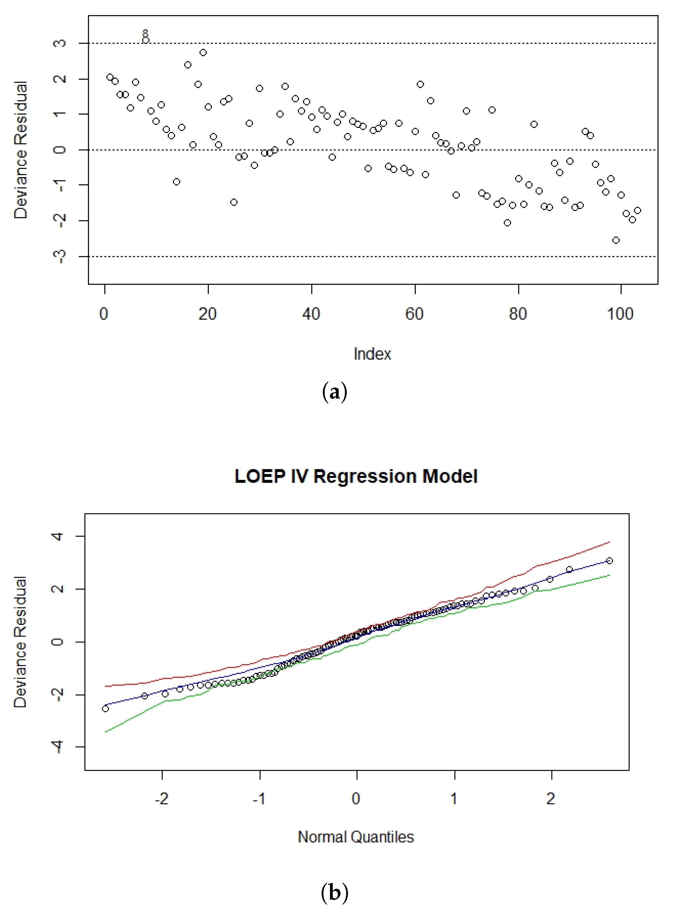
In order to detect possible outlaying observations, a plot for the versus the observations index is shown in Figure 10a. This demonstrated that almost all of the observations fall within (−3, 3), except for observation 8. Therefore, observation 8 was a possible outlier. Figure 10b shows the NPP for the deviance residuals with a generated envelope. Approximately all of the observations fell inside the envelope, which indicated that the proposed model was appropriate to fit the heart transplant data.
9. Concluding Remarks
In this article, we introduced the odd exponential-Pareto IV distribution. We derived some of its statistical and mathematical properties. The model parameters were estimated using the ML method, and simulation studies were carried out to examine the performance of the ML estimators based on biases and mean squared errors. Moreover, a new log-location regression model for censored data based on the OEPIV distribution was introduced. The ML and jackknife estimation methods for right censored data were used to estimate the unknown parameters of the new regression model. The model assumptions were checked using martingale and deviance residuals. Furthermore, generalized Cook and likelihood distance measures were defined to detect the influence observations for the regression model. Finally, we analyzed three real data sets to examine the usefulness of the OEPIV distribution and LOEPIV regression model. The results demonstrated that the OEPIV distribution outperformed other competitive distributions in terms of goodness of fit. In addition, the LOEPIV regression model provides a good fit for the Stanford heart transplant data.
Author Contributions
Conceptualization, L.A.B. and H.S.K.; methodology, L.A.B. and H.S.K.; software, L.A.B. and K.M.A.-B.; validation, L.A.B., H.S.K. and K.M.A.-B.; formal analysis, K.M.A.-B.; investigation of inference, H.S.K. and K.M.A.-B.; writing–original draft preparation, K.M.A.-B.; writing–review and editing, L.A.B. and H.S.K.; visualization, L.A.B., H.S.K. and K.M.A.-B.; supervision, L.A.B. and H.S.K. All authors have read and agreed to the published version of the manuscript.
Funding
This research received no external funding.
Acknowledgments
The authors would like to thank the referees and the editor for carefully reading the paper and for their great help in improving the paper.
Conflicts of Interest
The authors declare no conflict of interest.
References
- Burroughs, S.M.; Tebbens, S.F. Upper-truncated power laws in natural systems. Pure Appl. Geophys. 2001, 158, 741–757. [Google Scholar] [CrossRef]
- Schroeder, B.; Damouras, S.; Gill, P. Understanding latent sector errors and how to protect against them. ACM Trans. Storage (TOS) 2010, 6, 9. [Google Scholar] [CrossRef]
- Brazauskas, V. Information matrix for Pareto (IV), Burr, and related distributions. Commun. Stat. Theory Methods 2003, 32, 315–325. [Google Scholar] [CrossRef]
- Arnold, B. Pareto Distributions; International Co-operative Publishing House: Fairland, MD, USA, 1983. [Google Scholar]
- Pickands, J., III. Statistical inference using extreme order statistics. Ann. Stat. 1975, 3, 119–131. [Google Scholar]
- Akinsete, A.; Famoye, F.; Lee, C. The beta-Pareto distribution. Statistics 2008, 42, 547–563. [Google Scholar] [CrossRef]
- Mahmoudi, E. The beta generalized Pareto distribution with application to lifetime data. Math. Comput. Simul. 2011, 81, 2414–2430. [Google Scholar] [CrossRef]
- Alzaatreh, A.; Famoye, F.; Lee, C. Weibull-Pareto distribution and its applications. Commun. Stat. Theory Methods 2013, 42, 1673–1691. [Google Scholar] [CrossRef]
- Alzaatreh, A.; Famoye, F.; Lee, C. Gamma-Pareto distribution and its applications. J. Mod. Appl. Stat. Methods 2012, 11, 7. [Google Scholar] [CrossRef]
- Alzaatreh, A.; Ghosh, I. A study of the Gamma-Pareto (IV) distribution and its applications. Commun. Stat. Theory Methods 2016, 45, 636–654. [Google Scholar] [CrossRef]
- Elbatal, I. The Kumaraswamy exponentiated Pareto distribution. Econ. Qual. Control 2013, 28, 1–8. [Google Scholar] [CrossRef]
- Afify, A.Z.; Yousof, H.M.; Hamedani, G.; Aryal, G. The exponentiated Weibull-Pareto distribution with application. J. Stat. Theory Appl. 2016, 15, 328–346. [Google Scholar] [CrossRef] [Green Version]
- Cordeiro, G.M.; de Castro, M. A new family of generalized distributions. J. Stat. Comput. Simul. 2011, 81, 883–898. [Google Scholar] [CrossRef]
- Alexander, C.; Cordeiro, G.M.; Ortega, E.M.; Sarabia, J.M. Generalized beta-generated distributions. Comput. Stat. Data Anal. 2012, 56, 1880–1897. [Google Scholar] [CrossRef]
- Bourguignon, M.; Silva, R.B.; Cordeiro, G.M. The Weibull-G family of probability distributions. J. Data Sci. 2014, 12, 53–68. [Google Scholar]
- Ristić, M.M.; Balakrishnan, N. The gamma-exponentiated exponential distribution. J. Stat. Comput. Simul. 2012, 82, 1191–1206. [Google Scholar] [CrossRef]
- Afify, A.Z.; Yousof, H.M.; Butt, N.S.; Hamedani, G.G. The transmuted Weibull-Pareto distribution. Pakistan J. Stat. 2016, 32, 183–206. [Google Scholar]
- Ortega, E.M.; Lemonte, A.J.; Cordeiro, G.M.; Nilton da Cruz, J. The odd Birnbaum–Saunders regression model with applications to lifetime data. J. Stat. Theory Pract. 2016, 10, 780–804. [Google Scholar] [CrossRef]
- Jamal, F.; Nasir, M.A.; Tahir, M.; Montazeri, N.H. The odd Burr-III family of distributions. J. Stat. Appl. Probab. 2017, 6, 105–122. [Google Scholar] [CrossRef]
- Rosaiah, K.; Gadde, S.R.; Kalyani, K.; Charana Udaya Sivakumar, D. Odds Exponential Log Logistic Distribution: Properties and Estimation. J. Math. Stat. 2017, 13, 14–23. [Google Scholar] [CrossRef]
- Yousof, H.M.; Altun, E.; Hamedani, G. A New Extension Of FrÉChet Distribution With Regression Models, Residual Analysis And Characterizations. J. Data Sci. 2018, 16, 743–769. [Google Scholar]
- Altun, E.; Yousof, H.M.; Hamedani, G. A New Log-location Regression Model with Influence Diagnostics and Residual Analysis. Facta Univ. Ser. Math. Informat. 2018, 33, 417–449. [Google Scholar]
- Aldahlan, M.; Afify, A.Z. The odd exponentiated half-logistic Burr XII distribution. Pak. J. Stat. Oper. Res. 2018, 14, 305–317. [Google Scholar] [CrossRef] [Green Version]
- Cordeiro, G.M.; Afify, A.Z.; Ortega, E.M.; Suzuki, A.K.; Mead, M.E. The odd Lomax generator of distributions: Properties, estimation and applications. J. Comput. Appl. Math. 2019, 347, 222–237. [Google Scholar] [CrossRef]
- Afify, A.; Alizadeh, M. The Odd Dagum Family of Distributions: Properties and Applications. J. Appl. Probab. Stat. 2020, 15, 45–72. [Google Scholar]
- Alizadeh, M.; Afify, A.Z.; Eliwa, M.; Ali, S. The odd log-logistic Lindley-G family of distributions: Properties, Bayesian and non-Bayesian estimation with applications. Comput. Stat. 2020, 35, 281–308. [Google Scholar] [CrossRef]
- Alzaatreh, A.; Lee, C.; Famoye, F. A new method for generating families of continuous distributions. Metron 2013, 71, 63–79. [Google Scholar] [CrossRef] [Green Version]
- Lawless, J.F. Statistical Models and Methods for Lifetime Data; John Wiley & Sons: Hoboken, NJ, USA, 2011; Volume 362. [Google Scholar]
- Carrasco, J.M.; Ortega, E.M.; Paula, G.A. Log-modified Weibull regression models with censored data: Sensitivity and residual analysis. Comput. Stat. Data Anal. 2008, 52, 4021–4039. [Google Scholar] [CrossRef]
- Silva, G.O.; Ortega, E.M.; Cancho, V.G. Log-Weibull extended regression model: Estimation, sensitivity and residual analysis. Stat. Methodol. 2010, 7, 614–631. [Google Scholar] [CrossRef]
- Hashimoto, E.M.; Ortega, E.M.; Cancho, V.G.; Cordeiro, G.M. The log-exponentiated Weibull regression model for interval-censored data. Comput. Stat. Data Anal. 2010, 54, 1017–1035. [Google Scholar] [CrossRef]
- Hashimoto, E.M.; Ortega, E.M.; Cordeiro, G.M.; Barreto, M.L. The Log-Burr XII regression model for grouped survival data. J. Biopharm. Stat. 2012, 22, 141–159. [Google Scholar] [CrossRef]
- Ortega, E.M.; Cordeiro, G.M.; Kattan, M.W. The log-beta Weibull regression model with application to predict recurrence of prostate cancer. Stat. Pap. 2013, 54, 113–132. [Google Scholar] [CrossRef]
- Mahmoud, M.R.; EL-Sheikh, A.; Morad, N.A.; Ahmad, M.A. Log-beta log-logistic regression model. Int. J. Sci. Basic Appl. Res. (IJSBAR) 2015, 22, 389–405. [Google Scholar]
- Alamoudi, H.H.; Mousa, S.A.; Baharith, L.A. Estimation and application in log-Fréchet regression model using censored data. Int. J. Adv. Stat. Probab. 2017, 5, 23–31. [Google Scholar] [CrossRef] [Green Version]
- Al-Amoudi, H.H.; Mousa, S.A.; Baharith, L.A. Log-Exponentiated Frechet regression model with censored data. Int. J. Adv. Appl. Sci. 2016, 3, 1–9. [Google Scholar]
- Hashimoto, E.M.; Ortega, E.M.; Cordeiro, G.M.; Hamedani, G. The Log-gamma-logistic Regression Model: Estimation, Sensibility and Residual Analysis. J. Stat. Theory Appl. 2017, 16, 547–564. [Google Scholar] [CrossRef] [Green Version]
- Cruz, J.N.d.; Ortega, E.M.; Cordeiro, G.M. The log-odd log-logistic Weibull regression model: Modelling, estimation, influence diagnostics and residual analysis. J. Stat. Comput. Simul. 2016, 86, 1516–1538. [Google Scholar] [CrossRef]
- Pescim, R.R.; Ortega, E.M.; Cordeiro, G.M.; Alizadeh, M. A new log-location regression model: Estimation, influence diagnostics and residual analysis. J. Appl. Stat. 2017, 44, 233–252. [Google Scholar] [CrossRef]
- Ortega, E.M.; Cordeiro, G.M.; Hashimoto, E.M.; Cooray, K. A log-linear regression model for the odd Weibull distribution with censored data. J. Appl. Stat. 2014, 41, 1859–1880. [Google Scholar] [CrossRef]
- Al-Kadim, K.A.; Boshi, M.A. Exponential Pareto Distribution. Math. Theory Model. 2013, 3, 135–146. [Google Scholar]
- Sahinler, S.; Topuz, D. Bootstrap and jackknife resampling algorithms for estimation of regression parameters. J. Appl. Quant. Methods 2007, 2, 188–199. [Google Scholar]
- Algamal, Z.Y.; Rasheed, K.B. Re-sampling in Linear Regression Model Using Jackknife and Bootstrap. Iraqi J. Stat. Sci. 2010, 18, 59–73. [Google Scholar]
- Abdi, H.; WIlliams, L.J. Jackknife. Encyclopedia of Research Design 2; Salkind, N.J., Ed.; Sage: Thousand Oaks, CA, USA, 2010. [Google Scholar]
- Cook, R.D. Detection of influential observation in linear regression. Technometrics 1977, 19, 15–18. [Google Scholar]
- Barlow, W.E.; Prentice, R.L. Residuals for relative risk regression. Biometrika 1988, 75, 65–74. [Google Scholar] [CrossRef]
- Smith, R.L.; Naylor, J. A comparison of maximum likelihood and Bayesian estimators for the three-parameter Weibull distribution. J. R. Stat. Soc. Ser. C 1987, 36, 358–369. [Google Scholar] [CrossRef]
- Afify, A.Z.; Cordeiro, G.M.; Ortega, E.M.; Yousof, H.M.; Butt, N.S. The four-parameter Burr XII distribution: Properties, regression model, and applications. Commun. Stat. Theory Methods 2018, 47, 2605–2624. [Google Scholar] [CrossRef]
- Afify, A.Z.; Yousof, H.M.; Cordeiro, G.M.; Ortega, E.M.; Nofal, Z.M. The Weibull Fréchet distribution and its applications. J. Appl. Stat. 2016, 43, 2608–2626. [Google Scholar] [CrossRef]
- Tahir, M.H.; Cordeiro, G.M.; Mansoor, M.; Zubair, M. The Weibull-Lomax distribution: Properties and applications. Hacet. J. Math. Stat. 2015, 44, 461–480. [Google Scholar] [CrossRef]
- Tahir, M.H.; Cordeiro, G.M.; Alizadeh, M.; Mansoor, M.; Zubair, M.; Hamedani, G.G. The odd generalized exponential family of distributions with applications. J. Stat. Distrib. Appl. 2015, 2, 1. [Google Scholar] [CrossRef] [Green Version]
- Weisberg, S. Applied Linear Regression; John Wiley & Sons: Hoboken, NJ, USA, 2005; Volume 528. [Google Scholar]
- Tahir, M.; Cordeiro, G.M.; Mansoor, M. The Kumaraswamy Pareto IV Distribution. Austrian J. Stat. 2015. Available online: https://www.academia.edu/12965162/The_Kumaraswamy_Pareto_IV_distribution (accessed on 25 April 2020).
- Gupta, R.C.; Gupta, P.L.; Gupta, R.D. Modeling failure time data by Lehman alternatives. Commun. Stat. Theory Methods 1998, 27, 887–904. [Google Scholar] [CrossRef]
- Kalbfleisch, J.D.; Prentice, R.L. The Statistical Analysis of Failure Time Data; John Wiley & Sons: Hoboken, NJ, USA, 2011; Volume 360. [Google Scholar]
Figure 1.
Density function plots of the OEPIV distribution.

Figure 2.
Hazard function plots of the OEPIV distribution.

Figure 3.
Normal probability plots (NPP) for for different sample sizes (n) and censoring levels (c). (a) n = 30; c = 0.1 (b) n = 30; c = 0.3 (c) n = 30; c = 0.5 (d) n = 50; c = 0.1 (e) n = 50; c = 0.3 (f) n = 50; c = 0.5 (g) n = 100; c = 0.1 (h) n = 100; c = 0.3 (i) n = 100; c = 0.5.
Figure 3.
Normal probability plots (NPP) for for different sample sizes (n) and censoring levels (c). (a) n = 30; c = 0.1 (b) n = 30; c = 0.3 (c) n = 30; c = 0.5 (d) n = 50; c = 0.1 (e) n = 50; c = 0.3 (f) n = 50; c = 0.5 (g) n = 100; c = 0.1 (h) n = 100; c = 0.3 (i) n = 100; c = 0.5.

Figure 4.
NPP for for different sample sizes (n) and censoring levels (c). (a) n = 30; c = 0.1 (b) n = 30; c = 0.3 (c) n = 30; c = 0.5 (d) n = 50; c = 0.1 (e) n = 50; c = 0.3 (f) n = 50; c = 0.5 (g) n = 100; c = 0.1 (h) n = 100; c = 0.3 (i) n = 100; c = 0.5.
Figure 4.
NPP for for different sample sizes (n) and censoring levels (c). (a) n = 30; c = 0.1 (b) n = 30; c = 0.3 (c) n = 30; c = 0.5 (d) n = 50; c = 0.1 (e) n = 50; c = 0.3 (f) n = 50; c = 0.5 (g) n = 100; c = 0.1 (h) n = 100; c = 0.3 (i) n = 100; c = 0.5.


Figure 5.
QQ-plot of the OEPIV model and the estimated PDFs of the OEPIV and other competitive distributions for the glass fibers data.
Figure 5.
QQ-plot of the OEPIV model and the estimated PDFs of the OEPIV and other competitive distributions for the glass fibers data.

Figure 6.
QQ-plot of the OEPIV distribution and the estimated PDFs of the OEPIV and other competitive distributions for the skin folds data.
Figure 6.
QQ-plot of the OEPIV distribution and the estimated PDFs of the OEPIV and other competitive distributions for the skin folds data.

Figure 7.
Estimated SF based on the OEPIV distribution and the Kaplan–Meier (KM) model for the heart transplant data.
Figure 7.
Estimated SF based on the OEPIV distribution and the Kaplan–Meier (KM) model for the heart transplant data.

Figure 8.
Fitted SF from the LOEPIV regression model (a) for = age, (b) for = surgery, (c) for = transplant.
Figure 8.
Fitted SF from the LOEPIV regression model (a) for = age, (b) for = surgery, (c) for = transplant.


Figure 9.
The index plot of (a) and (b) for the LOEPIV regression model.

Figure 10.
The index plot of (a) the deviance residual and (b) the NPP for the deviance residual with envelopes.
Figure 10.
The index plot of (a) the deviance residual and (b) the NPP for the deviance residual with envelopes.


Table 1.
Mean, variance, skewness, and kurtosis of OEPIV model selected parameter values.
| a | Mean | Variance | Skewness | Kurtosis | |||
|---|---|---|---|---|---|---|---|
| 2 | 2.5 | 0.5 | 1.5 | 1.1281 | 23.5677 | 0.5281 | 0.0424 |
| 2 | 3.5 | 0.5 | 1.5 | 4.3493 | 192.0261 | 0.1223 | 0.0665 |
| 2 | 4.5 | 0.5 | 1.5 | 24.8511 | 488.3011 | 13.3934 | 7.6745 |
| 2 | 2.5 | 2.5 | 1.5 | 5.6405 | 589.1917 | 0.5281 | 0.0424 |
| 2 | 2.5 | 3.5 | 1.5 | 7.8967 | 1154.8158 | 0.5281 | 0.0424 |
| 2 | 2.5 | 0.5 | 1.5 | 1.1281 | 23.5677 | 0.5281 | 0.0424 |
| 0.5 | 2.5 | 1.5 | 1.5 | 1.1153 | 5.3631 | 0.7241 | 0.4752 |
| 0.5 | 2.5 | 1.5 | 2.5 | 0.9486 | 9.6007 | 0.0298 | 0.0131 |
| 0.5 | 2.5 | 1.5 | 4.5 | 0.8567 | 13.2012 | 0.0302 | 0.0084 |
| 1.5 | 3.5 | 0.5 | 1.5 | 3.0317 | 47.0037 | 0.5800 | 0.3771 |
| 2.5 | 3.5 | 0.5 | 1.5 | 7.7388 | 568.5549 | 0.1148 | 0.0424 |
| 3.5 | 3.5 | 0.5 | 1.5 | 42.8019 | 1795.2542 | 4.7337 | 2.5407 |
Table 2.
Parameter estimates, along with their MSE, and bias for two different cases with different sample sizes.
Table 2.
Parameter estimates, along with their MSE, and bias for two different cases with different sample sizes.
| Set I | Set II | ||||||
|---|---|---|---|---|---|---|---|
| Estimate | MSE | Bias | Estimate | MSE | Bias | ||
| 0.7646 | 34.3149 | 0.4646 | 0.4444 | 1.1410 | 0.2444 | ||
| a | 0.1806 | 0.1159 | −0.2194 | 0.0347 | 0.0086 | −0.0653 | |
| 1.0773 | 1009.5916 | 0.5773 | 0.6595 | 0.0570 | 0.0595 | ||
| 0.0778 | 0.0364 | −0.1222 | 0.0440 | 0.0374 | −0.1060 | ||
| 0.5774 | 1.1837 | 0.2774 | 0.3526 | 0.4563 | 0.1526 | ||
| a | 0.2333 | 0.0893 | −0.1667 | 0.0495 | 0.0074 | −0.0505 | |
| 0.6825 | 0.7605 | 0.1825 | 0.6366 | 0.0235 | 0.0366 | ||
| 0.1008 | 0.0228 | −0.0992 | 0.0631 | 0.0161 | −0.0869 | ||
| 0.4324 | 0.3672 | 0.1324 | 0.2628 | 0.0909 | 0.0628 | ||
| a | 0.3072 | 0.0540 | −0.0928 | 0.0683 | 0.0051 | −0.0317 | |
| 0.6042 | 0.2970 | 0.1042 | 0.6147 | 0.0132 | 0.0147 | ||
| 0.1430 | 0.0128 | −0.0570 | 0.0953 | 0.0105 | −0.0547 | ||
| 0.3535 | 0.0982 | 0.0535 | 0.2243 | 0.0221 | 0.0243 | ||
| a | 0.3532 | 0.0256 | −0.0468 | 0.0830 | 0.0028 | −0.0170 | |
| 0.5463 | 0.1018 | 0.0463 | 0.6054 | 0.0064 | 0.0054 | ||
| 0.1718 | 0.0057 | −0.0282 | 0.1211 | 0.0058 | −0.0289 | ||
| 0.3156 | 0.0140 | 0.0156 | 0.2069 | 0.0038 | 0.0069 | ||
| a | 0.3847 | 0.0082 | −0.0153 | 0.0942 | 0.0010 | −0.0058 | |
| 0.5149 | 0.0211 | 0.0149 | 0.6015 | 0.0020 | 0.0015 | ||
| 0.1911 | 0.0017 | −0.0089 | 0.1403 | 0.0020 | −0.0097 | ||
Table 3.
Maximum likelihood (ML) estimates, SE in (), , and Akaike information criterion (AIC) and corrected Akaike Information Criterion (CAIC) statistics for the glass fibers data.
Table 3.
Maximum likelihood (ML) estimates, SE in (), , and Akaike information criterion (AIC) and corrected Akaike Information Criterion (CAIC) statistics for the glass fibers data.
| Distribution | ML Estimate and SE in () | AIC | CAIC | ||||
|---|---|---|---|---|---|---|---|
| OEPIV | = 0.0401 | a = 0.2862 | = 1.1455 | = 2.1549 | 13.9507 | 35.902 | 36.591 |
| (0.0810) | (0.1368) | (0.4016) | ((1.4014) | ||||
| WBXII | a = 0.0026 | b = 1.8888 | = 1.6077 | = 2.7409 | 14.3035 | 36.607 | 37.297 |
| (0.0032) | (0.7680) | (0.3760) | (1.0100) | ||||
| WL | a = 581.4052 | b = 5.1752 | = 17.5336 | = 110.7104 | 14.934 | 37.868 | 38.558 |
| (28.2900) | (0.2010) | (102.1130) | (659.3920) | ||||
| WFr | a = 1.4762 | b = 16.8561 | = 0.3865 | = 0.2436 | 15.5005 | 39.001 | 39.691 |
| (4.7820) | (20.4850) | (0.7990) | (0.2850) | ||||
| Pareto IV | a = 0.1626 | = 2.3513 | = 10.2153 | - | 15.4781 | 36.956 | 37.363 |
| (0.0187) | (0.4477) | (9.9080) | |||||
| OE-W | = 0.0721 | = 1.9603 | - | - | 16.4613 | 36.922 | 37.123 |
| (0.0162) | (0.0940) | ||||||
| OE-N | = 0.0121 | = 0.7385 | - | - | 17.5979 | 39.195 | 39.396 |
| (0.0043) | (0.0364) | ||||||
| Gamma | = 17.4411 | = 11.5748 | - | - | 23.9515 | 51.9031 | 52.1031 |
| (3.0783) | (2.0725) | ||||||
Table 4.
ML estimates, SE in (), , and AIC and CAIC statistics for skin folds data.
| Distribution | ML Estimate and SE in () | AIC | CAIC | |||||
|---|---|---|---|---|---|---|---|---|
| OEPIV | = 0.348 | a = 0.024 | = 29.579 | = 0.036 | - | 944.2687 | 1896.537 | 1896.740 |
| (0.090) | (0.006) | (0.678) | (0.010) | |||||
| KwPIV | a = 2.928 | b = 21.746 | = 0.023 | = 0.060 | = 23.430 | 945.200 | 1900.401 | 1900.707 |
| (1.188) | (33.283) | (0.019) | (0.033) | (4.633) | ||||
| GPIV | c = 0.520 | = 81.355 | = 0.098 | - | - | 950.007 | 1906.014 | 1906.135 |
| (0.198) | (8.071) | (0.035) | ||||||
| PIV | = 0.463 | = 0.182 | = 46.812 | - | - | 956.333 | 1918.666 | 1918.787 |
| (0.183) | (0.041) | (5.595) | ||||||
| EP | c = 28 | = 2.155 | = 2.737 | - | - | 951.878 | 1907.757 | 1907.878 |
| (0.154) | (0.298) | |||||||
| Weibull | = 2.2635 | = 78.2664 | - | - | - | 975.2427 | 1954.485 | 1954.545 |
| (0.1159) | (2.5832) | |||||||
Table 5.
The ML estimates, SE in (), p-values in [], AIC, CAIC, and ayesian Information Criterion (BIC) statistics of the log odds exponential-Pareto IV (LOEPIV), log-exponentiated Fréchet (LEF), log-odd log-logistic Weibull (LOLLW), log-Fréchet (LF), log-Weibull (LW), and log exponential-Pareto (LEP) regression models for the heart transplant data.
| Models | AIC | CAIC | BIC | |||||||
|---|---|---|---|---|---|---|---|---|---|---|
| 1.3754 | 0.1257 | 0.5569 | 3.5186 | −0.0539 | 1.7494 | 2.5405 | 343.42 | 344.61 | 361.87 | |
| LOEPIV | (1.9087) | (0.0974) | (0.1689) | (1.0747) | (0.0192) | (0.5524) | (0.3621) | |||
| [0.00106] | [0.00507] | [0.00154] | [<0.001] | |||||||
| - | 6.2746 | 3.5882 | 8.6744 | −0.0624 | 0.8910 | 2.7241 | 346.72 | 347.59 | 362.53 | |
| LEF | - | (7.5737) | (1.4492) | (3.5491) | (0.0206) | (0.5059) | (0.3780) | |||
| - | - | - | [0.016] | [0.002] | [0.078] | [<0.001] | ||||
| - | 4.62831 | 6.20325 | 8.74485 | −0.07692 | 1.40550 | 2.59196 | 347.59 | 348.47 | 363.40 | |
| LOLLW | - | (3.5307) | (4.6851) | (1.7603) | (0.0199) | (0.5745) | (0.3884) | |||
| - | - | - | [<0.001] | [<-0.001] | [0.016] | [<0.001] | ||||
| - | - | 1.7457 | 4.2129 | −0.0431 | 0.6902 | 2.6572 | 349.15 | 349.77 | 362.33 | |
| LF | - | - | (0.1484) | (0.9153) | (0.0189) | (0.5034) | (0.3782) | |||
| - | - | - | [<0.001] | [0.023] | [0.170] | [<0.001] | ||||
| - | - | 1.4658 | 7.9742 | −0.0924 | 1.2143 | 2.5375 | 353.42 | 354.03 | 366.59 | |
| LW | - | - | (0.13148) | (0.93397) | (0.02061) | (0.64700) | (0.37336) | |||
| - | - | - | [<0.001] | [<0.001] | [0.063] | [<0.001] | ||||
| 0.1439 | - | 1.4655 | 5.1321 | −0.0923 | 1.214127 | 2.537713 | 355.42 | 356.29 | 371.22 | |
| LEP | (1.1088) | - | (0.1314) | (11.3276) | (0.0206) | (0.6469) | (0.3733) | |||
| - | - | - | [0.6505] | [<0.001] | [0.061] | [<0.001] |
Table 6.
LR statistic for heart transplant.
| Heart Transplant | Hypotheses | Statistic w | p-Values | |
|---|---|---|---|---|
| LOEPIV vs. LEP | versus is not true | 13.9922 | 0.00018 | |
Table 7.
The Jackknife parameter estimates of the LOEPIV regression model.
| Parameter | Estimate | SE | 95% Confidence Intervals |
|---|---|---|---|
| 1.4043 | 1.5262 | (0.0000, 4.3957) | |
| 0.0838 | 0.0988 | (0.0000, 0.2775) | |
| 0.6586 | 0.1885 | (0.2891, 1.0281) | |
| 3.8616 | 1.1072 | (1.6915, 6.031) | |
| -0.0536 | 0.0196 | (−0.0921, −0.0152) | |
| 1.7304 | 0.5262 | (0.6989, 2.7619) | |
| 2.5563 | 0.3881 | (1.7955, 3.3172) |
© 2020 by the authors. Licensee MDPI, Basel, Switzerland. This article is an open access article distributed under the terms and conditions of the Creative Commons Attribution (CC BY) license (http://creativecommons.org/licenses/by/4.0/).
Share and Cite
MDPI and ACS Style
Baharith, L.A.; AL-Beladi, K.M.; Klakattawi, H.S. The Odds Exponential-Pareto IV Distribution: Regression Model and Application. Entropy 2020, 22, 497. https://doi.org/10.3390/e22050497
AMA Style
Baharith LA, AL-Beladi KM, Klakattawi HS. The Odds Exponential-Pareto IV Distribution: Regression Model and Application. Entropy. 2020; 22(5):497. https://doi.org/10.3390/e22050497
Chicago/Turabian StyleBaharith, Lamya A., Kholod M. AL-Beladi, and Hadeel S. Klakattawi. 2020. "The Odds Exponential-Pareto IV Distribution: Regression Model and Application" Entropy 22, no. 5: 497. https://doi.org/10.3390/e22050497
Note that from the first issue of 2016, this journal uses article numbers instead of page numbers. See further details here.