
Tsallis Entropy for Loss Models and Survival Models Involving Truncated and Censored Random Variables
by
 , , and
Vasile Preda
1,2,3,
Silvia Dedu
2,4,* ,
,
Iuliana Iatan
5,
Ioana Dănilă Cernat
3 and
and
Muhammad Sheraz
6,7 1
“Gheorghe Mihoc-Caius Iacob” Institute of Mathematical Statistics and Applied Mathematics, 050711 Bucharest, Romania
2
“Costin C. Kiriţescu” National Institute of Economic Research, 050711 Bucharest, Romania
3
Faculty of Mathematics and Computer Science, University of Bucharest, Academiei 14, 010014 Bucharest, Romania
4
Department of Applied Mathematics, Bucharest University of Economic Studies, 010734 Bucharest, Romania
5
Department of Mathematics and Computer Science, Technical University of Civil Engineering, 020396 Bucharest, Romania
6
Institute of Business Administration Karachi, Department of Mathematical Sciences, School of Mathematics and Computer Science, Karachi 75270, Pakistan
7
Department Financial Mathematics, Fraunhofer ITWM, Fraunhofer-Platz, 67663 Kaiserslautern, Germany
*
Author to whom correspondence should be addressed.
Entropy 2022, 24(11), 1654; https://doi.org/10.3390/e24111654
Submission received: 25 August 2022
/
Revised: 11 November 2022
/
Accepted: 11 November 2022
/
Published: 14 November 2022
(This article belongs to the Special Issue Measures of Information II)
Abstract
:The aim of this paper consists in developing an entropy-based approach to risk assessment for actuarial models involving truncated and censored random variables by using the Tsallis entropy measure. The effect of some partial insurance models, such as inflation, truncation and censoring from above and truncation and censoring from below upon the entropy of losses is investigated in this framework. Analytic expressions for the per-payment and per-loss entropies are obtained, and the relationship between these entropies are studied. The Tsallis entropy of losses of the right-truncated loss random variable corresponding to the per-loss risk model with a deductible d and a policy limit u is computed for the exponential, Weibull, or Gamma distribution. In this context, the properties of the resulting entropies, such as the residual loss entropy and the past loss entropy, are studied as a result of using a deductible and a policy limit, respectively. Relationships between these entropy measures are derived, and the combined effect of a deductible and a policy limit is also analyzed. By investigating residual and past entropies for survival models, the entropies of losses corresponding to the proportional hazard and proportional reversed hazard models are derived. The Tsallis entropy approach for actuarial models involving truncated and censored random variables is new and more realistic, since it allows a greater degree of flexibility and improves the modeling accuracy.
1. Introduction
Risk assessment represents an important topic in various fields, since it allows designing the optimal strategy in many real-world problems. The fundamental concept of entropy can be used to evaluate the uncertainty degree corresponding to the result of an experiment, phenomenon or random variable. Recent research results in statistics prove the increased interest for using different entropy measures. Many authors have dealt with this matter, among them are Koukoumis and Karagrigoriou [1], Iatan et al. [2], Li et al. [3], Miśkiewicz [4], Toma et. al. [5], Moretto et al. [6], Remuzgo et al. [7], Sheraz et al. [8] and Toma and Leoni-Aubin [9]. One of the most important information measures, the Tsallis entropy, has attracted considerable interest in statistical physics and many other fields as well. We can mention here the contributions of Nayak et al. [10], Pavlos et al. [11] and Singh and Cui [12]. Recently, Balakrishnan et al. [13] proposed a general formulation of a class of entropy measures depending on two parameters, which includes Shannon, Tsallis and fractional entropy as special cases.
As entropy can be regarded as a measure of variability for absolutely continuous random variables or measure of variation or diversity of the possible values of a discrete random variable, it can be used for risk assessment in various domains. In actuarial science, one of the main objectives which defines the optimal strategy of an insurance company is directed towards minimizing the risk of the claims. Ebrahimi [14] and Ebrahimi and Pellerey [15] studied the problem of measuring uncertainty in life distributions. The uncertainty corresponding to loss random variables in actuarial models can be evaluated also by the entropy of the loss distribution. Frequently in actuarial practice, as a consequence of using deductibles and policy limits, the practitioners have to deal with transformed data, generated by truncation and censoring. Baxter [16] and Zografos [17] developed information measure methods for mixed and censored random variables, respectively. The entropic approach enables the assessment of the uncertainty degree for loss models involving truncated and censored random variables. Sachlas and Papaioannou [18] investigated the effect of inflation, truncation or censoring from below or above on the Shannon entropy of losses of insurance policies. In this context of per-payment and per-loss models, they derived analytic formulas for the Shannon entropy of actuarial models involving several types of partial insurance coverage and studied the properties of the resulting entropies. Recent results in this field have also been obtained by Gupta and Gupta [19] and Di Crescenzo and Longobardi [20], Meselidis and Karagrigoriou [21].
This paper aims to develop several entropy-based risk models involving truncated and censored loss random variables. In this framework, the effect of some partial insurance schemes, such truncation and censoring from above, truncation and censoring from below and inflation is investigated using the Tsallis entropy. The paper is organized as follows. In Section 2 some preliminary results are presented. In Section 3 representation formulas for the Tsallis entropy corresponding to the truncated and censored loss random variables in the per-payment and per-loss approach are derived, and the relationships between these entropies are obtained. Moreover, the combined effect of a deductible and a policy limit is investigated. In Section 4, closed formulas for the Tsallis entropy corresponding to some survival models are derived, including the proportional hazard and the proportional reversed hazard models. Some concluding remarks are provided in the last section.
2. Preliminaries
2.1. The Exponential Distribution
An exponential distributed random variable is defined by the probability density function:
with and the cumulative distribution function:
2.2. The Weibull Distribution
A Weibull distributed random variable is closely related to an exponential distributed random variable and has the probability density function:
with > 0.
If , then the Weibull distribution can be generated using the formula:
2.3. The Distribution
Let be independent random variables, Gaussian distributed and . A random variable with degrees of freedom can be represented as:
A distributed random variable with degrees of freedom is represented by the probability density function:
where denotes the Euler Gamma function.
2.4. The Gamma Distribution
An exponential distributed random variable is defined by the probability density function [22]:
where are, respectively, the location parameter, the scale parameter and the form parameter of the variable X.
We can notice that an exponential distributed random variable is a gamma random variable ) and a distributed random variable is a gamma distributed random variable .
If and , then we have:
2.5. The Tsallis Entropy
Entropy represents a fundamental concept which can be used to evaluate the uncertainty associated with a random variable or with the result of an experiment. It provides information regarding the predictability of the results of a random variable X. The Shannon entropy, along with other measures of information, such as the Renyi entropy, may be interpreted as a descriptive quantity of the corresponding probability density function.
Entropy can be regarded as a measure of variability for absolutely continuous random variables or as a measure of variation or diversity of the possible values of discrete random variables. Due to the widespread applicability and use of information measures, the derivation of explicit expressions for various entropy and divergence measures corresponding to univariate and multivariate distributions has been a subject of interest; see, for example, Pardo [23], Toma [24], Belzunce et al. [25], Vonta and Karagrigoriou [26]. Various measures of entropy and generalizations thereof have been proposed in the literature.
The Tsallis entropy was introduced by Constantino Tsallis in 1988 [27,28,29,30] with the aim of generalizing the standard Boltzmann–Gibbs entropy and, since then, it has attracted considerable interest in the physics community, as well as outside it. Recently, Furuichi [31,32] investigated information theoretical properties of the Tsallis entropy and obtained a uniqueness theorem for the Tsallis entropy. The use of Tsallis entropy enhances the analysis and solving of some important problems regarding financial data and phenomena modeling, such as the distribution of asset returns, derivative pricing or risk aversion. Recent research in statistics increased the interest in using Tsallis entropy. Trivellato [33,34] used the minimization of the divergence corresponding to the Tsallis entropy as a criterion to select a pricing measure in the valuation problems of incomplete markets and gave conditions on the existence and on the equivalence to the basic measure of the minimal k–entropy martingale measure. Preda et al. [35,36] used Tsallis and Kaniadakis entropies to construct the minimal entropy martingale for semi-Markov regime switching interest rate models and to derive new Lorenz curves for modeling income distribution. Miranskyy et al. [37] investigated the application of some extended entropies, such as Landsberg–Vedral, Rényi and Tsallis entropies to the classification of traces related to various software defects.
Let X be a real-valued discrete random variable defined on the probability space , with the probability mass function . Let . We introduce the definition of Tsallis entropy [27] for discrete and absolutely continuous random variables in terms of expected value operator with respect to a probability measure.
Definition 1.
The Tsallis entropy corresponding to the discrete random variable X is defined by:
where represents the expected value operator with respect to the probability mass function .
Let X be a real-valued continuous random variable defined on the probability space , with the probability density function . Let .
Definition 2.
The Tsallis entropy corresponding to the continuous random variable X is defined by:
provided that the integral exists, where represents the expected value operator with respect to the probability density function .
In the sequel, we suppose to know the properties of the expected value operator, such as additivity and homogeneity.
Note that for , the Tsallis entropy reduces to the second-order entropy [38] and for , we obtain the Shannon entropy [39]. The real parameter was introduced in the definition of Tsallis entropy for evaluating more accurately the degree of uncertainty. In this regard, the Tsallis parameter tunes the importance assigned to rare events in the considered model.
Highly uncertain insurance policies are less reliable. The uncertainty for the loss associated to an insurance policy can be quantified by using the entropy of the corresponding loss distribution. In the actuarial practice, frequently transformed data are available as a consequence of deductibles and liability limits. Recent research in statistics increased the interest for using different entropy measures for risk assessment.
3. Tsallis Entropy Approach for Loss Models
We denote by X the random variable which models the loss corresponding to an insurance policy. We suppose that X is non-negative and denote by and its probability density function and cumulative distribution function, respectively. Let be the survival function of the random variable X, defined by .
We consider truncated and censored random variables obtained from X, which can be used to model situations which frequently appear in actuarial practice as a consequence of using deductibles and policy limits. In the next subsections, analytical expressions for the Tsallis entropy are derived, corresponding to the loss models based on truncated and censored random variables.
3.1. Loss Models Involving Truncation or Censoring from Below
Loss models with left-truncated or censored from below random variables are used when losses are not recorded or reported below a specified threshold, mainly as a result of applying deductible policies. We denote by d the value of the threshold, referred to as the deductible value. According to Kluggman et al. [40], there are two approaches used to express the random variable which models the loss, corresponding to the per-payment and per-loss cases, respectively.
In the per-payment case, losses or claims below the value of the deductible may not be reported to the insurance company, generating truncated from below or left-truncated data.
We denote by the left-truncated random variable which models the loss corresponding to an insurance policy with a deductible d in the per-payment case. It can be expressed as , or equivalently:
In order to investigate the effect of truncation from bellow, we use the Tsallis entropy for evaluating uncertainty corresponding to the loss covered by the insurance company. The following theorem establishes the relationship between the Tsallis entropy of the random variables X and . We denote by the per-payment Tsallis entropy with a deductible d.
We denote by the indicator function of the set A, defined by:
In the sequel, the integrals are always supposed to be correctly defined.
Theorem 1.
Let X be a non-negative random variable which models the loss corresponding to an insurance policy. Let and . The Tsallis entropy of the left-truncated loss random variable corresponding to the per-payment risk model with a deductible d can be expressed as follows:
Proof.
The probability density function of the random variable is given by , . Therefore, the Tsallis entropy of the random variable can be expressed as follows:
□
Remark 1.
For the limiting case , we obtain the corresponding results for the Shannon entropy from [18].
In the per-loss case corresponding to an insurance policy with a deductible d, all the claims are reported, but only the ones over the deductible value are paid. As only the real losses of the insurer are taken into consideration, this situation generates censored from below data.
We denote by the left-censored random variable which models the loss corresponding to an insurance policy with a deductible d in the per-loss case. As X is censored from below at point d, it results that the random variable can be expressed as follows:
We note that assigns a positive probability mass at zero point, corresponding to the case . In this case, it not absolutely continuous, but a mixed random variable, consisting of a discrete and a continuous part. We can remark that the per-payment loss random variable can be expressed as the per-loss one given that the later is positive.
In the next theorem, the relation between the Tsallis entropy of the random variables X and is established.
Theorem 2.
Let X be a non-negative random variable which models the loss corresponding to an insurance policy. Let and . The Tsallis entropy of the left-censored loss random variable corresponding to the per-payment risk model with a deductible d can be expressed as follows:
Proof.
The Tsallis entropy of , which is a mixed random variable consisting of a discrete part at zero and a continuous part over , is given by:
and the conclusion follows. □
Remark 2.
Let and . Then,
It results that the Tsallis entropy of the left-censored loss random variable corresponding to the per-loss risk model is greater than the Tsallis entropy of the loss random variable, and the difference can be quantified by the right-hand side of the formula above.
Let , and . Let X be Exp distributed and denoted by . Using Theorem 2, we obtain
Figure 1 displays the graph of function for and different values of the Tsallis entropy parameter .
Theorem 3.
Let X be a non-negative random variable which models the loss corresponding to an insurance policy. Let . The Tsallis entropy measures and are connected through the following relationship:
where represents a Bernoulli distributed random variable with parameter .
Proof.
By multiplying (13) with , we obtain:
From Theorem 2, we have:
By subtracting the two relations above, we obtain:
□
Now, we denote by , for , the hazard rate function of the random variable X. In the next theorem, the per-payment simple or residual entropy with a deductible d is expressed in terms of the hazard or risk function of X.
Theorem 4.
Let X be a non-negative random variable which models the loss corresponding to an insurance policy. Let . The Tsallis entropy of the left-truncated loss random variable corresponding to the per-payment risk model with a deductible d is given by:
Proof.
From Theorem 1, we have:
We have:
Integrating by parts the second term from the relation above, we obtain:
Hence,
□
Theorem 5.
Let X be a non-negative random variable which models the loss corresponding to an insurance policy. Let . The Tsallis entropy of the left-truncated loss random variable corresponding to the per-loss risk model with a deductible d is independent of d if, and only if, the hazard rate function is constant.
Proof.
We assume that the hazard function is constant, therefore , for any . It results that , for any and, using (17), we obtain:
which does not depend on d.
Conversely, assuming that does not depend on d,
Using again the hypothesis that does not depend on d, it follows that does not depend on d, therefore is constant. □
3.2. Loss Models Involving Truncation or Censoring from Above
Right-truncated or censored from below random variables are used in actuarial models with policy limits. In this case, losses are not recorded or reported for or above a specified threshold. We denote by the value of the threshold, referred to as the policy limit or liability limit. According to Kluggman et. al [40], there are two approaches used to express the random variable which models the loss corresponding to the per-payment and per-loss cases, respectively.
In the per-payment case, losses or claims above the value of the liability limit may not be reported to the insurance company, generating truncated from above or right-truncated data.
We denote by the right-truncated random variable which models the loss corresponding to an insurance policy limit u in the per-payment case. It can be expressed as , or equivalently:
The relationship between the Tsallis entropy of the random variables X and is established in the following theorem.
Theorem 6.
Let X be a non-negative random variable which models the loss corresponding to an insurance policy. Let . The Tsallis entropy of the right-truncated loss random variable corresponding to the per-payment risk model with a policy limit u is given by:
Proof.
The probability density function of the random variable is given by , . Therefore, the Tsallis entropy of the random variable can be expressed as follows:
□
In the following theorem, the Tsallis entropy of the right-truncated loss random variable corresponding to the per-payment risk model with a policy limit is derived.
Theorem 7.
Let X be a non-negative random variable which models the loss corresponding to an insurance policy. Let and . The Tsallis entropy of the right-truncated loss random variable corresponding to the per-payment risk model with a policy limit u can be expressed in terms of the reversed hazard function as follows:
Proof.
The probability density function of the random variable is given by , . Therefore, the Tsallis entropy of the random variable can be expressed as follows:
□
Now, we consider the case of the per-loss right censoring. In this case, if the loss exceeds the value of the policy limit, the insurance company pays an amount u.
For example, a car insurance policy covers losses up to a limit u, while major losses are covered by the car owner. If the loss is modeled by the random variable X, then the loss corresponding to the insurance company is represented by . We note that the loss model with truncation from above is different from the loss model with censoring from above, which is defined by the random variable . In this case, if the loss is , the insurance company pays an amount u.
The loss model with censoring from above is modeled using the random variable . Moreover, it can be represented as
This model, corresponding to the per-loss case, assumes that in the case where the loss is , the insurance company pays an amount u. Therefore, the insurer pays a maximum amount of u on a claim. We note that the random variable is not absolutely continuous.
In the following theorem, an analytical formula for the entropy corresponding to the random variable is obtained.
Theorem 8.
Let X be a non-negative random variable which models the loss corresponding to an insurance policy. Let and . The Tsallis entropy of losses for the right-censored loss random variable corresponding to the per-payment risk model with a policy limit u can be expressed as follows:
Proof.
We have:
□
3.3. Loss Models Involving Truncation from Above and from Below
We denote by d the deductible and by u the retention limit, with . The deductible is applied after the implementation of the retention limit u. Therefore, if the value of the loss is grater than u, then the value of the maximum payment is . We denote by the loss random variable which models the payments to the policy holder under a combination of deductible and retention limit policies. is a mixed random variable, with an absolutely continuous part over the interval and two discrete parts at 0, with probability mass and at and with probability mass . Following [40], the loss random variable can be expressed by:
The deductible d is applied after the implementation of the retention limit u, which means that if the loss is greater than u, then the maximum payment is . The random variable is a mixed variable with an absolutely continuous part over the interval and two discrete parts at 0, with probability mass and at and with probability mass .
In the next theorem, the Tsallis entropy of losses for the right-truncated loss random variable corresponding to the per-loss risk model with a deductible d and a policy limit u is derived.
Theorem 9.
Let X be a non-negative random variable which models the loss corresponding to an insurance policy. Let , and . The Tsallis entropy of losses of the right-truncated loss random variable corresponding to the per-loss risk model with a deductible d and a policy limit u is given by:
Proof.
The probability density function of the random variable is given by
where denotes the Dirac delta function.
It results:
□
The following theorem establishes the relationship between , the entropy under censoring from above and the entropy under censoring from below .
Theorem 10.
Let X be a non-negative random variable which models the loss corresponding to an insurance policy. Let . For any and , the Tsallis entropy is related to the entropies and through the following relationship:
Proof.
We have:
Moreover,
It results that:
□
Figure 2 illustrates the Tsallis entropy of the right-truncated loss random variable , corresponding to the per-loss risk model with a deductible d and a policy limit u for the exponential distribution with .
Figure 2 displays a similar behavior of the Tsallis entropy for all the considered values around 1 of the parameter. Thus, we remark that, for all values of , the Tsallis entropy is decreasing with respect to the deductible d and it does not depend on the policy limit u.
Figure 3 represents the Tsallis entropy of losses for the right-truncated loss random variable corresponding to the per-loss risk model with a deductible d and a policy limit u for the distribution, with and for different values of the Tsallis parameter , in the case .
Figure 3 reveals, for all the values of the parameter considered, a similar decreasing behavior with respect to the deductible d of the Tsallis entropy . Moreover, it indicates that the Tsallis entropy does not depend on the values of the policy limit u.
Figure 4 depicts the Tsallis entropy of losses of the right-truncated loss random variable corresponding to the per-loss risk model with a deductible d and a policy limit u for the Weibull distribution, with and for different values of the Tsallis parameter , in the case .
Figure 4 highlights that the Tsallis entropy of losses is decreasing with respect to d for all the values of the parameter considered. Moreover, the Tsallis entropy does not depend on the policy limit u for the values of the parameter around 1, respectively, for and . A different behavior is detected for . In this case, we remark that the Tsallis entropy is increasing with respect to the policy limit u, which is realistic from the actuarial point of view. Indeed, increasing the policy limit results in a higher risk for the insurance company.
The conclusions obtained indicate that Tsallis entropy measures with parameter values significantly different from 1 can provide a better loss model involving truncation from above and from below.
Figure 5 displays the Tsallis entropy of losses for the right-truncated loss random variable corresponding to the per-loss risk model with a deductible d and a policy limit u for the Gamma distribution, with and for different values of the Tsallis parameter , in the case .
Figure 5 reveals the decreasing behavior of the Tsallis entropy of losses for all the values of the Tsallis parameter considered. Moreover, for all the values of , the Tsallis entropy does not depend on the policy limit u.
The following tables present the Tsallis entropy values for the Weibull distribution, corresponding to the analyzed models.
Table 1 illustrates the Tsallis entropy values in case of the Weibull distribution with and for different values of the Tsallis parameter and several values of the policy limit u.
The analysis of the results presented in Table 1 reveals that for parameter values the Tsallis entropy corresponding to the random variable is increasing with respect to the value of the policy limit u. On the other side, for , the Tsallis entropy, which reduces to the Shannon entropy measure, is decreasing with respect to u. From an actuarial perspective, when the policy limit increases, the risk of the insurance company also increases, therefore the entropy of losses increases, too. The detected behavior of the Tsallis entropy measure is reasonable in this case, and it means that the Tsallis entropy approach for evaluating the risk corresponding to the random variable is more realistic.
Table 2 displays the values of the Tsallis entropy measures in case of the Weibull distribution with and for different values of the Tsallis parameter and several values of the policy limit u.
Analyzing the results presented in Table 2, we remark that for parameter values the Tsallis entropy corresponding to the random variable is increasing with respect to the value of the policy limit u. On the other side, for , the Tsallis entropy, which reduces to the Shannon entropy measure, is decreasing with respect to u. From an actuarial perspective, when the policy limit increases, the risk of the insurance company also increases, therefore the entropy of losses increases, too. The detected behavior of the Tsallis entropy measure is reasonable in this case, and it means that the Tsallis entropy approach for evaluating the risk corresponding to the random variable is more realistic.
Table 3 illustrates the Tsallis entropy values in the case of the Weibull distribution with and deductible for various values of the Tsallis parameter and several values of the policy limit u.
The study of the results presented in Table 3 reveals that for parameter values the Tsallis entropy corresponding to the random variable is increasing with respect to the value of the policy limit u. On the other side, for , the Tsallis entropy, which reduces to the Shannon entropy measure, is decreasing with respect to u. From an actuarial perspective, when the policy limit increases, the risk of the insurance company also increases, therefore the entropy of losses increases, too. The detected behavior of the Tsallis entropy measure is reasonable in this case, and it means that the Tsallis entropy approach for evaluating the risk corresponding to the random variable is more realistic.
Table 4 reveals the values of all the Tsallis entropy measures analyzed in the case of the Weibull distribution with and for several values of the Tsallis parameter and different values of the policy limit u.
The results displayed in Table 4 show that for the Tsallis entropy of the random variable increases with respect to the value of the policy limit u, whereas for , the entropy decreases with respect to u. It indicates that, when the policy limit increases, the risk of the insurance company increases, too. Thus, the entropy of losses is increasing. We can also conclude that in this case the right-truncated loss random variable is better modeled using Tsallis entropy measure.
Table 5 displays the Tsallis entropy values in case of the Weibull distribution with and deductible for different values of the Tsallis parameter and several values of the policy limit u.
Analyzing the results provided in Table 5, we remark that for the parameter the Tsallis entropy corresponding to the right-truncated random variable is increasing with respect to the value of the policy limit u. For , the Shannon entropy measure decreases with respect to u. From an actuarial perspective, when the policy limit increases, the risk of the insurance company also increases, therefore the entropy of losses increases, too. The detected behavior of the Tsallis entropy measure is reasonable in this case, and it means that the Tsallis entropy approach for evaluating the risk corresponding to the random variable is more realistic.
From Table 1, Table 2, Table 3, Table 4 and Table 5, we draw the following conclusions. Using the Tsallis entropy measure approach, in the case when the deductible value d increases, the uncertainty of losses for the insurance company will decrease, therefore the company has to pay smaller amounts. In the case when the policy limit value u increases, the uncertainty of losses for the insurance company will increase, as the company has to pay greater amounts. Therefore, the Tsallis entropy approach is more realistic and flexible, providing a relevant perspective and a useful instrument for loss models.
3.4. Loss Models under Inflation
Financial and actuarial models are estimated using observations made in the past years. As inflation implies an increase in losses, the models must be adjusted corresponding to the current level of loss experience. Moreover, a projection of the anticipated losses in the future needs to be performed.
Now, we study the effect of inflation on entropy. Let X be the random variable that models the loss corresponding to a certain year. We denote by F the cumulative distribution function of X and by f the probability density function of X. The random variable that models the loss after one year and under the inflation effect is , where , represents the annual inflation rate. We denote by the cumulative distribution function of and by the probability density function of the random variable .
The probability density function corresponding to the random variable is given by:
The following theorem derives the relationship between the Tsallis entropies of the random variables X and .
Theorem 11.
Let X be a non-negative random variable which models the loss corresponding to an insurance policy. Let . The Tsallis entropy of the random variable , which models the loss after one year under inflation rate r, , is given by
Proof.
Using the definition of the Tsallis entropy, we have:
Using the change in variable given by , it follows
□
Theorem 12.
Let X be a non-negative random variable which models the loss corresponding to an insurance policy. Let . For , the Tsallis entropy of the random variable , which models the loss after one year under inflation rate , is always larger than that of X and is an increasing function of r.
Proof.
Let . We denote by
We have:
so that is an increasing function of r.
Therefore, it follows that
□
The results obtained show that inflation increases the entropy, which means that the uncertainty degree of losses increases compared with the case without inflation. Moreover, the uncertainty of losses increases with respect to the inflation rate.
4. Tsallis Entropy Approach for Survival Models
In this section, we derive residual and past entropy expressions for some survival models, including the proportional hazard and the proportional reversed hazard models. Relevant results in this field have been obtained by Sachlas and Papaioannou [18], Gupta and Gupta [19], Di Crescenzo [41] and Sankaran and Gleeja [42].
Let X and Y be random variables with cumulative distribution functions F and G, probability density functions f and g and survival functions and , respectively. We denote by and the hazard rate functions of the random variables X and Y, respectively.
4.1. The Proportional Hazard Rate Model
Definition 3.
The random variables X and Y satisfy the proportional hazard rate model if there exists such that (see Cox [43]).
We note that the random variables X and Y satisfy the proportional hazard rate model if the hazard rate function of Y is proportional to the hazard rate function of X, i.e., for every ; see Cox [43].
In the next theorem, the Tsallis entropy of the left-truncated random variable under the proportional hazard rate model is derived.
Theorem 13.
Let X and Y be non-negative random variables. Let and . Under the proportional hazard rate model given in (28), the Tsallis entropy of the left-truncated random variable corresponding to the per-payment risk model with a deductible d can be expressed as follows:
Proof.
□
4.2. The Proportional Reversed Hazard Rate Model
Definition 4.
The random variables X and Y satisfy the proportional reversed hazard rate model [43] if there exists such that
In the next theorem, the Tsallis entropy of the right-truncated random variable under the proportional reversed hazard rate model is derived.
Theorem 14.
Let X and Y be non-negative random variables. Let and . Under the proportional reversed hazard rate model given in (30), the Tsallis entropy of the right-truncated random variable corresponding to the per-payment risk model with a policy limit u can be expressed as follows:
5. Applications
We used a real database from [18], representing the Danish fire insurance losses recorded during the 1980–1990 period [44,45,46], where losses are ranged from MDKK 1.0 to 263.250 (millions of Danish Krone). The average loss is MDKK 3.385, while of losses are smaller than MDKK 1.321 and of losses are smaller than MDKK 2.967.
The data from the database [18] were fitted by using a Weibull distribution and the maximum likelihood estimators of the shape , and scale parameters of the distribution were obtained.
The results displayed in Table 1, Table 2, Table 3, Table 4 and Table 5 can be used to compare the values of the following entropy measures:
- The Tsallis entropy corresponding to the random variable X which models the loss;
- The Tsallis entropy of the left-truncated loss and, respectively, censored loss random variable corresponding to the per-payment risk model with a deductible d, namely and, respectively, ;
- The Tsallis entropy of the right-truncated and, respectively, censored loss random variable corresponding to the per-payment risk model with a policy limit u, denoted by and, respectively, ;
- The Tsallis entropy of losses of the right-truncated loss random variable corresponding to the per-loss risk model with a deductible d and a policy limit u, .
In the case of the Weibull distribution, for the parameter values and for and for different values of the Tsallis entropy parameter located in the neighborhood of the point 1, we draw the following conclusions. The values of the Tsallis entropy for correspond to those obtained in [18]. Moreover, we remark that, for values of the Tsallis parameter lower than 1, the values of the corresponding entropy measures increase. Moreover, for values of the parameter greater than 1, the values of the corresponding entropy measures decrease, as we can notice from Figure 3, too. This behavior allows a higher degree of flexibility for modeling the loss-truncated and loss-censored random variables in actuarial models.
6. Conclusions
In this paper, an entropy-based approach for risk assessment in the framework of loss models and survival models involving truncated and censored random variables was developed.
By using the Tsallis entropy, the effect of some partial insurance schemes, such as inflation, truncation and censoring from above and truncation and censoring from below was investigated.
Analytical expressions for the per-payment and per-loss entropies of losses were derived. Moreover, closed formulas for the entropy of losses corresponding to the proportional hazard rate model and the proportional reversed hazard rate model were obtained.
The results obtained point out that entropy depends on the deductible and the policy limit, and inflation increases entropy, which means the increase in the uncertainty degree of losses increases compared with the case without inflation. The use of entropy measures allows risk assessment for actuarial models involving truncated and censored random variables.
We used a real database representing the Danish fire insurance losses recorded between 1980 and 1990 [44,45,46], where losses range from MDKK 1.0 to 263.250 (millions of Danish Krone). The average loss is MDKK 3.385, while of losses are smaller than MDKK 1.321 and of losses are smaller than MDKK 2.967.
The data were fitted using the Weibull distribution in order to obtain the maximum likelihood estimators of the shape and scale parameters of the distribution .
The values of the Tsallis entropies for correspond to those from [18], while as the is lower than 1 the values of the entropies will increase and, as the is bigger than 1, the values of the entropies will decrease, as we can notice from the Figure 3, too.
The paper extends several results obtained in this field; see, for example, Sachlas and Papaioannou [18].
The study of the results obtained reveals that for parameter values the Tsallis entropy corresponding to the right-truncated loss random variable is increasing with respect to the value of the policy limit u. On the other side, for , the Tsallis entropy, which reduces to the Shannon entropy measure, is decreasing with respect to u. From an actuarial perspective, when the policy limit increases, the risk of the insurance company also increases, therefore the entropy of losses increases, too. The detected behavior proves that the Tsallis entropy approach for evaluating the risk corresponding to the right-truncated loss random variable is more realistic.
Therefore, we can conclude that the Tsallis entropy approach for actuarial models involving truncated and censored random variables provides a new and relevant perspective, since it allows a higher degree of flexibility for the assessment of risk models.
Author Contributions
All authors contributed equally to the paper. All authors have read and agreed to the published version of the manuscript.
Funding
This work was supported by a grant of the Romanian Ministery of Education and Research, CNCS—UEFISCDI, project number PN-III-P4-ID-PCE-2020-1112, within PNCDI III.
Institutional Review Board Statement
Not applicable.
Informed Consent Statement
Not applicable.
Data Availability Statement
Not applicable.
Acknowledgments
The authors would like to express their gratitude to the anonymous referees for their valuable suggestions and comments.
Conflicts of Interest
The authors declare no conflict of interest.
References
- Koukoumis, C.; Karagrigoriou, A. On Entropy-type Measures and Divergences with Applications in Engineering, Management and Applied Sciences. Int. J. Math. Eng. Manag. Sci. 2021, 6, 688–707. [Google Scholar] [CrossRef]
- Iatan, I.; Dragan, M.; Preda, V.; Dedu, S. Using Probabilistic Models for Data Compression. Mathematics 2022, 10, 3847. [Google Scholar] [CrossRef]
- Li, S.; Zhuang, Y.; He, J. Stock market stability: Diffusion entropy analysis. Phys. A 2016, 450, 462–465. [Google Scholar] [CrossRef]
- Miśkiewicz, J. Improving quality of sample entropy estimation for continuous distribution probability functions. Phys. A 2016, 450, 473–485. [Google Scholar] [CrossRef]
- Toma, A.; Karagrigoriou, A.; Trentou, P. Robust Model Selection Criteria Based on Pseudodistances. Entropy 2020, 22, 304. [Google Scholar] [CrossRef] [PubMed] [Green Version]
- Moretto, E.; Pasquali, S.; Trivellato, E. Option pricing under deformed Gaussian distributions. Phys. A 2016, 446, 246–263. [Google Scholar] [CrossRef]
- Remuzgo, L.; Trueba, C.; Sarabia, S.M. Evolution of the global inequality in greenhouse gases emissions using multidimensional generalized entropy measures. Phys. A 2015, 444, 146–157. [Google Scholar] [CrossRef] [Green Version]
- Sheraz, M.; Dedu, S.; Preda, V. Volatility Dynamics of Non-Linear Volatile Time Series and Analysis of Information Flow: Evidence from Cryptocurrency Data. Entropy 2022, 24, 1410. [Google Scholar] [CrossRef]
- Toma, A.; Leoni-Aubin, S. Robust portfolio optimization using pseudodistances. PLoS ONE 2015, 10, e0140546. [Google Scholar] [CrossRef] [Green Version]
- Nayak, A.S.; Rajagopal, S.A.K.; Devi, A.R.U. Bipartite separability of symmetric N-qubit noisy states using conditional quantum relative Tsallis entropy. Phys. A 2016, 443, 286–295. [Google Scholar] [CrossRef]
- Pavlos, G.P.; Iliopoulos, A.C.; Zastenker, G.N.; Zelenyi, L.M. Tsallis non-extensive statistics and solar wind plasma complexity. Phys. A 2015, 422, 113–135. [Google Scholar] [CrossRef]
- Singh, V.P.; Cui, H. Suspended sediment concentration distribution using Tsallis entropy. Phys. A 2014, 414, 31–42. [Google Scholar] [CrossRef]
- Balakrishnan, N.; Buono, F.; Longobardi, M. A unified formulation of entropy and its application. Phys. A 2022, 596, 127214. [Google Scholar] [CrossRef]
- Ebrahimi, N. How to measure uncertainty in the residual life distributions. Sankhya 1996, 58, 48–57. [Google Scholar]
- Ebrahimi, N.; Pellerey, F. New partial ordering of survival functions based on the notion of uncertainty. J. Appl. Probab. 1995, 32, 202–211. [Google Scholar] [CrossRef]
- Baxter, L.A. A note on information and censored absolutely continuous random variables. Stat. Decis. 1989, 7, 193–197. [Google Scholar] [CrossRef]
- Zografos, K. On some entropy and divergence type measures of variability and dependence for mixed continuous and discrete variables. J. Stat. Plan. Inference 2008, 138, 3899–3914. [Google Scholar] [CrossRef]
- Sachlas, A.; Papaioannou, T. Residual and past entropy in actuarial science. Methodol. Comput. Appl. Probab. 2014, 16, 79–99. [Google Scholar] [CrossRef]
- Gupta, R.C.; Gupta, R.D. Proportional reversed hazard rate model and its applications. J. Stat. Plan. Inference 2007, 137, 3525–3536. [Google Scholar] [CrossRef]
- Di Crescenzo, A.; Longobardi, M. Entropy-based measure of uncertainty in past lifetime distributions. J. Appl. Probab. 2002, 39, 430–440. [Google Scholar] [CrossRef]
- Messelidis, C.; Karagrigoriou, A. Contingency Table Analysis and Inference via Double Index Measures. Entropy 2022, 24, 477. [Google Scholar] [CrossRef] [PubMed]
- Anastassiou, G.; Iatan, I.F. Modern Algorithms of Simulation for Getting Some Random Numbers. J. Comput. Anal. Appl. 2013, 15, 1211–1222. [Google Scholar]
- Pardo, L. Statistical Inference Based on Divergence Meaures; Chapman & Hall/CRC: Boca Raton, FL, USA, 2006. [Google Scholar]
- Toma, A. Model selection criteria using divergences. Entropy 2014, 16, 2686–2698. [Google Scholar] [CrossRef] [Green Version]
- Belzunce, F.; Navarro, J.; Ruiz, J.; del Aguila, Y. Some results on residual entropy function. Metrika 2004, 59, 147–161. [Google Scholar] [CrossRef]
- Vonta, F.; Karagrigoriou, A. Generalized measures of divergence in survival analysis and reliability. J. Appl. Probab. 2010, 47, 216–234. [Google Scholar] [CrossRef] [Green Version]
- Tsallis, C. Possible generalization of Boltzmann–Gibbs statistics. J. Stat. Phys. 1988, 52, 479–487. [Google Scholar] [CrossRef]
- Tsallis, C.; Mendes, R.S.; Plastino, A.R. The role of constraints within generalized nonextensive statistics. Phys. A 1998, 261, 534–554. [Google Scholar] [CrossRef]
- Tsallis, C.; Anteneodo, A.; Borland, L.; Osorio, R. Nonextensive statistical mechanics and economics. Phys. A 2003, 324, 89–100. [Google Scholar] [CrossRef] [Green Version]
- Tsallis, C. Introduction to Nonextensive Statistical Mechanics; Springer Science Business Media, LLC: Berlin/Heidelberg, Germany, 2009. [Google Scholar]
- Furuichi, S. Information theoretical properties of Tsallis entropies. J. Math. Phys. 2006, 47, 023302. [Google Scholar] [CrossRef] [Green Version]
- Furuichi, S. On uniqueness theorems for Tsallis entropy and Tsallis relative entropy. IEEE Trans. Inf. Theory 2005, 51, 3638–3645. [Google Scholar] [CrossRef] [Green Version]
- Trivellato, B. Deformed exponentials and applications to finance. Entropy 2013, 15, 3471–3489. [Google Scholar] [CrossRef] [Green Version]
- Trivellato, B. The minimal k-entropy martingale measure. Int. J. Theor. Appl. Financ. 2012, 15, 1250038. [Google Scholar] [CrossRef]
- Preda, V.; Dedu, S.; Sheraz, M. New measure selection for Hunt-Devolder semi-Markov regime switching interest rate models. Phys. A 2014, 407, 350–359. [Google Scholar] [CrossRef]
- Preda, V.; Dedu, S.; Gheorghe, C. New classes of Lorenz curves by maximizing Tsallis entropy under mean and Gini equality and inequality constraints. Phys. A 2015, 436, 925–932. [Google Scholar] [CrossRef]
- Miranskyy, A.V.; Davison, M.; Reesor, M.; Murtaza, S.S. Using entropy measures for comparison of software traces. Inform. Sci. 2012, 203, 59–72. [Google Scholar] [CrossRef] [Green Version]
- Preda, V.; Dedu, S.; Sheraz, M. Second order entropy approach for risk models involving truncation and censoring. Proc. Rom.-Acad. Ser. Math. Phys. Tech. Sci. Inf. Sci. 2016, 17, 195–202. [Google Scholar]
- Shannon, C.E. A mathematical theory of communication. BellSyst. Tech. J. 1984, 27, 379–423. [Google Scholar]
- Klugman, S.A.; Panjer, H.H.; Willmot, G.E. Loss Models: From Data to Decisions; John Wiley and Sons: New York, NY, USA, 2004. [Google Scholar]
- Di Crescenzo, A. Some results on the proportional reversed hazards model. Stat. Probab. Lett. 2000, 50, 313–321. [Google Scholar] [CrossRef]
- Sankaran, P.G.; Gleeja, C.L. Proportional reversed hazard and frailty models. Metrika 2008, 68, 333–342. [Google Scholar] [CrossRef]
- Cox, D.R. Regression models and life-tables. J. R. Stat. Soc. 1972, 34, 187–220. [Google Scholar] [CrossRef]
- McNeil, A.J. Estimating the tails of loss severity distributions using extreme value theory. ASTIN Bull. 1997, 27, 117–137. [Google Scholar] [CrossRef] [Green Version]
- Pigeon, M.; Denuit, M. Composite Lognormal-Pareto model with random threshold. Scand. Actuar. J. 2011, 3, 177–192. [Google Scholar] [CrossRef]
- Resnick, S.I. Discussion of the Danish data on large fire insurance losses. ASTIN Bull. 1997, 27, 139–151. [Google Scholar] [CrossRef]
Figure 1.
The graph for and different values of the Tsallis entropy parameter .
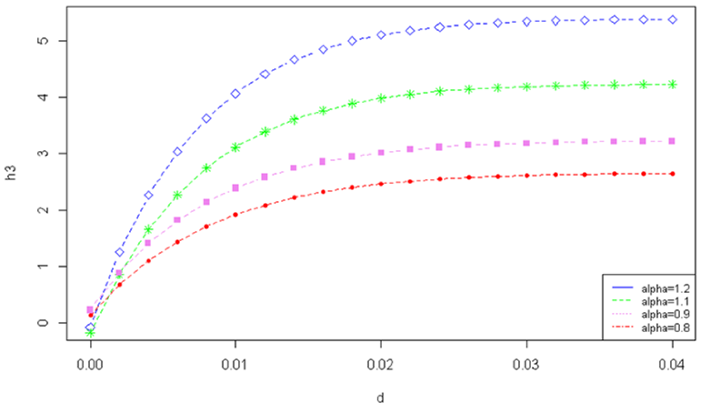
Figure 2.
The Tsallis entropy of losses for the right-truncated loss random variable corresponding to the per-loss risk model with a deductible d and a policy limit u for the exponential distribution, with and different values of the Tsallis parameter .
Figure 2.
The Tsallis entropy of losses for the right-truncated loss random variable corresponding to the per-loss risk model with a deductible d and a policy limit u for the exponential distribution, with and different values of the Tsallis parameter .
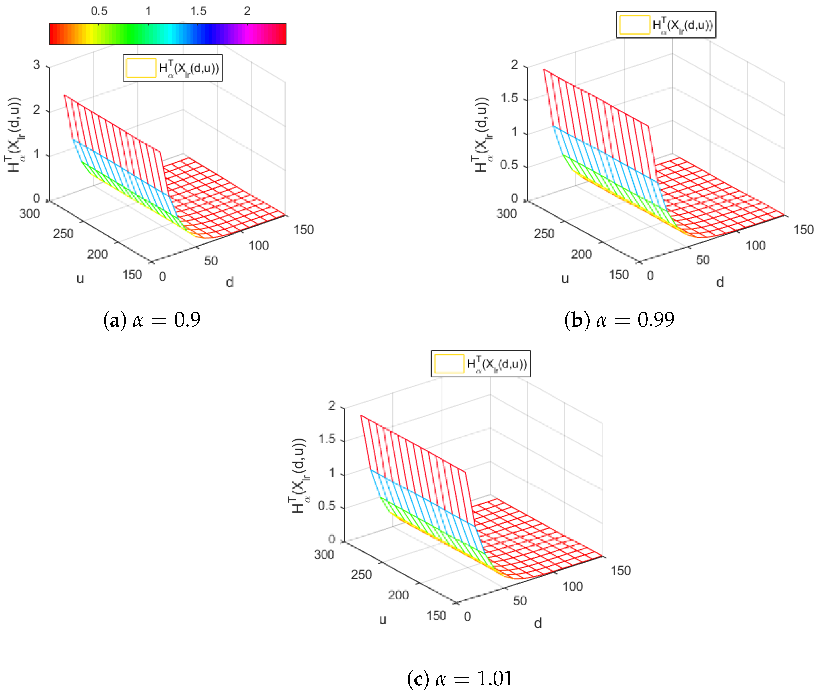
Figure 3.
The Tsallis entropy of losses of the right-truncated loss random variable corresponding to the per-loss risk model with a deductible d and a policy limit u for the distribution, with and different values of the Tsallis parameter .
Figure 3.
The Tsallis entropy of losses of the right-truncated loss random variable corresponding to the per-loss risk model with a deductible d and a policy limit u for the distribution, with and different values of the Tsallis parameter .
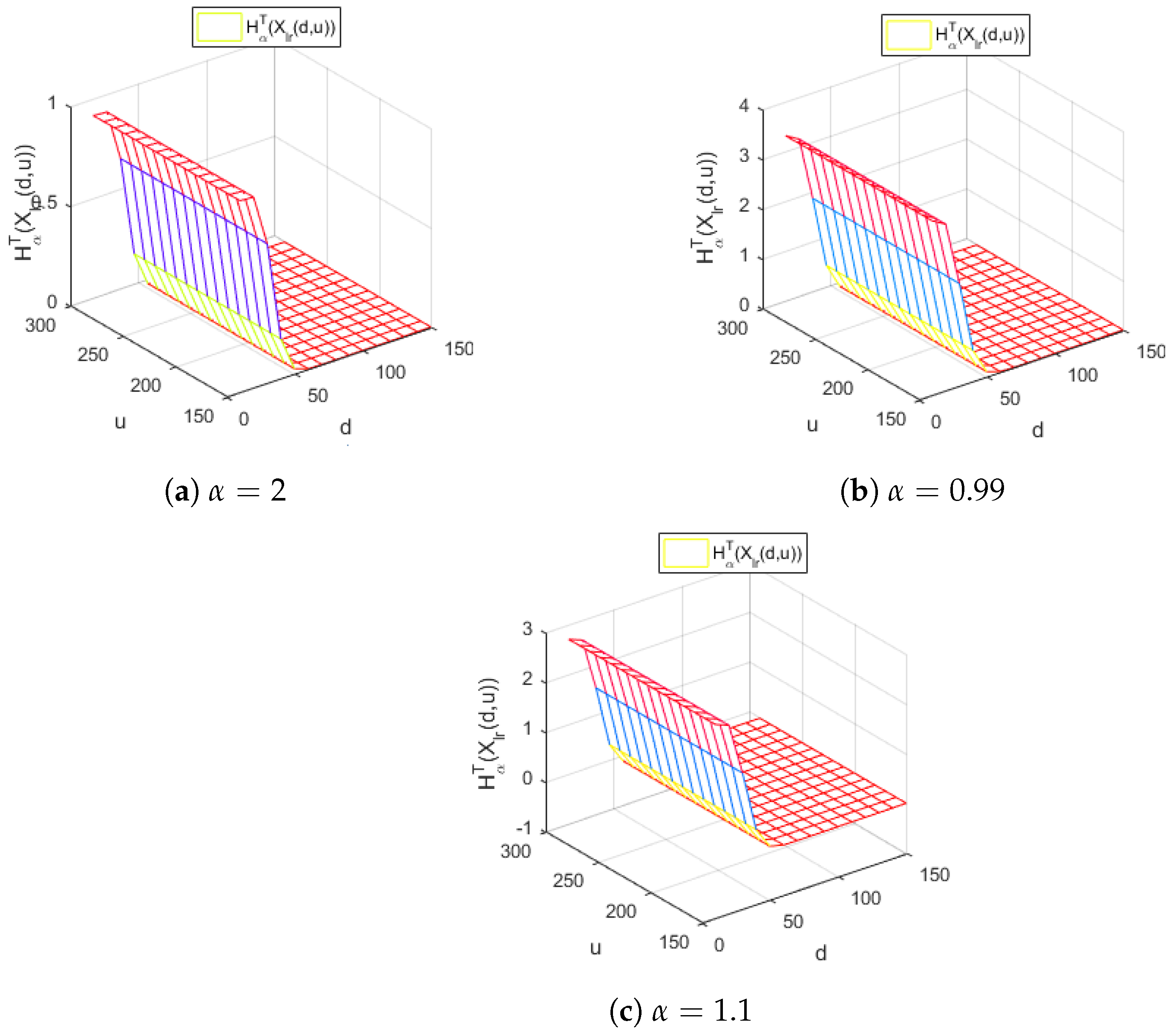
Figure 4.
The Tsallis entropy of losses of the right-truncated loss random variable corresponding to the per-loss risk model with a deductible d and a policy limit u for the Weibull distribution, with and different values of the Tsallis parameter .
Figure 4.
The Tsallis entropy of losses of the right-truncated loss random variable corresponding to the per-loss risk model with a deductible d and a policy limit u for the Weibull distribution, with and different values of the Tsallis parameter .
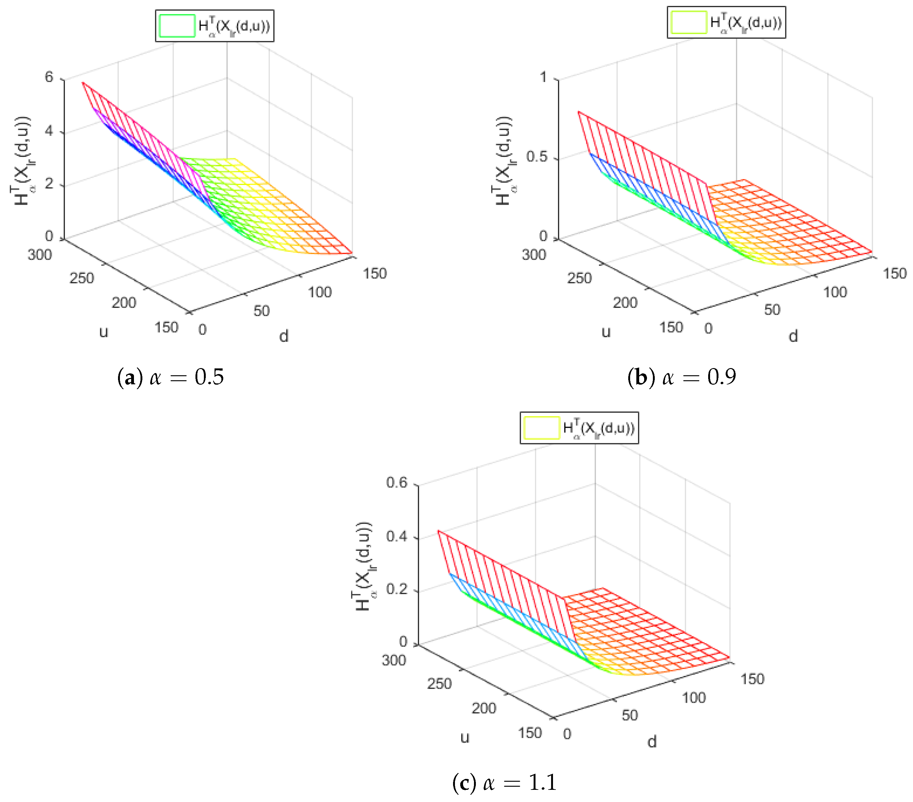
Figure 5.
The Tsallis entropy of losses of the right-truncated loss random variable corresponding to the per-loss risk model with a deductible d and a policy limit u for the Gamma distribution, with and different values of the Tsallis parameter .
Figure 5.
The Tsallis entropy of losses of the right-truncated loss random variable corresponding to the per-loss risk model with a deductible d and a policy limit u for the Gamma distribution, with and different values of the Tsallis parameter .


Table 1.
Tsallis entropy values for the Weibull distribution for: .
| u | |||||||
|---|---|---|---|---|---|---|---|
| 10 | 5.434 | 5.5005 | 5.3837 | 3.7994 | 4.1067 | 4.0564 | |
| 0.5 | 15 | 4.5725 | 4.7622 | 4.712 | |||
| 20 | 4.9845 | 5.09140 | 5.0411 | ||||
| 25 | 5.2006 | 5.2582 | 5.2079 | ||||
| 10 | 2.5446 | 2.5778 | 2.5156 | 2.2220 | 2.3504 | 2.3214 | |
| 0.9 | 15 | 2.4306 | 2.488 | 2.4591 | |||
| 20 | 2.505432 | 2.52792 | 2.4989660524 | ||||
| 25 | 2.5156 | 2.5314 | 2.5396 | ||||
| 10 | 2.20865 | 2.2369 | 1.091 | 2.316 | 2.0827 | 2.0792 | |
| 1 | 15 | 2.2534 | 2.1767 | 2.1732 | |||
| 20 | 2.22484 | 2.20041 | 2.1969 | ||||
| 25 | 2.2140 | 2.2064 | 2.203 | ||||
| 10 | 1.26474 | 1.278 | 1.2521 | 1.2094 | 1.24799 | 1.2353 | |
| 1.5 | 15 | 1.2503 | 1.2626 | 1.2499 | |||
| 20 | 1.2609475715 | 1.2644 | 1.2518 | ||||
| 25 | 1.2637 | 1.2647 | 1.2525 | ||||
| 10 | 0.8459 | 0.8524 | 0.8396 | 0.8279 | 0.8433 | 0.837 | |
| 2 | 15 | 0.8415 | 0.8457 | 0.83944 | |||
| 20 | 0.8448 | 0.8459 | 0.8395 | ||||
| 25 | 0.8456 | 0.8459 | 0.8396 |
Table 2.
Tsallis entropy values for the Weibull distribution for: .
| u | |||||||
|---|---|---|---|---|---|---|---|
| 10 | 5.434 | 5.5043 | 5.33 | 3.7994 | 4.1067 | 4.0027 | |
| 0.5 | 15 | 4.5725 | 4.7622 | 4.6583 | |||
| 20 | 4.98457 | 5.091 | 4.9874 | ||||
| 25 | 5.2006 | 5.2582 | 5.1542 | ||||
| 10 | 2.5446 | 2.5796 | 2.4829 | 2.222 | 2.35 | 2.2887 | |
| 0.9 | 15 | 2.43 | 2.488 | 2.4264 | |||
| 20 | 2.5054 | 2.5279 | 2.4662 | ||||
| 25 | 2.5314 | 2.5396 | 2.4779 | ||||
| 10 | 2.20865 | 2.2384 | 1.0621 | 2.31601 | 2.0827 | 2.09548 | |
| 1 | 15 | 2.2534 | 2.1767 | 2.1894 | |||
| 20 | 2.2248 | 2.2004 | 2.2131 | ||||
| 25 | 2.214 | 2.2064 | 2.2192 | ||||
| 10 | 1.26474 | 1.2786 | 1.2364 | 1.2094 | 1.2479 | 1.2197 | |
| 1.5 | 15 | 1.2503 | 1.2626 | 1.2343 | |||
| 20 | 1.2609 | 1.2644 | 1.2362 | ||||
| 25 | 1.26373 | 1.2647 | 1.2364 | ||||
| 10 | 0.8459 | 0.85275 | 0.8311 | 0.82792 | 0.8433 | 0.8285 | |
| 2 | 15 | 0.8415 | 0.8457 | 0.8309 | |||
| 20 | 0.8448 | 0.8459 | 0.8395 | ||||
| 25 | 0.8448 | 0.8459 | 0.8311 |
Table 3.
Tsallis entropy values for the Weibull distribution for: .
| u | |||||||
|---|---|---|---|---|---|---|---|
| 10 | 5.434 | 5.508 | 5.2754 | 3.7994 | 4.1067 | 3.9481 | |
| 0.5 | 15 | 4.5725 | 4.7622 | 4.6036 | |||
| 20 | 4.9845 | 5.0914 | 4.9328 | ||||
| 25 | 5.2006 | 5.2582 | 5.0996 | ||||
| 10 | 2.5446 | 2.5812 | 2.4491 | 2.222 | 2.3504 | 2.2549 | |
| 0.9 | 15 | 2.4306 | 2.488 | 2.3926 | |||
| 20 | 2.5054 | 2.5279 | 2.4324 | ||||
| 25 | 2.5314 | 2.5396 | 2.4441 | ||||
| 10 | 2.2086 | 2.2398 | 1.03212 | 2.316 | 2.08275 | 2.11294 | |
| 1 | 15 | 2.2534 | 2.1767 | 2.20691 | |||
| 20 | 2.2248 | 2.2004 | 2.23 | ||||
| 25 | 2.214 | 2.2064 | 2.2366 | ||||
| 10 | 1.2647 | 1.2792 | 1.2199 | 1.2094 | 1.2479 | 1.2031 | |
| 1.5 | 15 | 1.2503 | 1.2626 | 1.2178 | |||
| 20 | 1.2609 | 1.2644 | 1.2196 | ||||
| 25 | 1.2637 | 1.2647 | 1.2199 | ||||
| 10 | 0.8459 | 0.853 | 0.8219 | 0.8279 | 0.8433 | 0.8193 | |
| 2 | 15 | 0.8415 | 0.8457 | 0.8218 | |||
| 20 | 0.8448 | 0.8459 | 0.8219 | ||||
| 25 | 0.8456 | 0.8459 | 0.8219 |
Table 4.
Tsallis entropy values for the Weibull distribution for: .
| u | |||||||
|---|---|---|---|---|---|---|---|
| 10 | |||||||
| 0.5 | 15 | ||||||
| 20 | |||||||
| 25 | |||||||
| 10 | |||||||
| 0.9 | 15 | ||||||
| 20 | |||||||
| 25 | |||||||
| 10 | |||||||
| 1 | 15 | ||||||
| 20 | |||||||
| 25 | |||||||
| 10 | |||||||
| 1.5 | 15 | ||||||
| 20 | |||||||
| 25 | |||||||
| 10 | |||||||
| 2 | 15 | ||||||
| 20 | |||||||
| 25 |
Table 5.
Tsallis entropy values for the Weibull distribution for: and .
| u | |||||||
|---|---|---|---|---|---|---|---|
| 10 | |||||||
| 0.5 | 15 | ||||||
| 20 | |||||||
| 25 | |||||||
| 10 | |||||||
| 0.9 | 15 | ||||||
| 20 | |||||||
| 25 | |||||||
| 10 | |||||||
| 1 | 15 | ||||||
| 20 | |||||||
| 25 | |||||||
| 10 | |||||||
| 1.5 | 15 | ||||||
| 20 | |||||||
| 25 | |||||||
| 10 | |||||||
| 2 | 15 | ||||||
| 20 | |||||||
| 25 |
Publisher’s Note: MDPI stays neutral with regard to jurisdictional claims in published maps and institutional affiliations. |
© 2022 by the authors. Licensee MDPI, Basel, Switzerland. This article is an open access article distributed under the terms and conditions of the Creative Commons Attribution (CC BY) license (https://creativecommons.org/licenses/by/4.0/).
Share and Cite
MDPI and ACS Style
Preda, V.; Dedu, S.; Iatan, I.; Cernat, I.D.; Sheraz, M. Tsallis Entropy for Loss Models and Survival Models Involving Truncated and Censored Random Variables. Entropy 2022, 24, 1654. https://doi.org/10.3390/e24111654
AMA Style
Preda V, Dedu S, Iatan I, Cernat ID, Sheraz M. Tsallis Entropy for Loss Models and Survival Models Involving Truncated and Censored Random Variables. Entropy. 2022; 24(11):1654. https://doi.org/10.3390/e24111654
Chicago/Turabian StylePreda, Vasile, Silvia Dedu, Iuliana Iatan, Ioana Dănilă Cernat, and Muhammad Sheraz. 2022. "Tsallis Entropy for Loss Models and Survival Models Involving Truncated and Censored Random Variables" Entropy 24, no. 11: 1654. https://doi.org/10.3390/e24111654
Note that from the first issue of 2016, this journal uses article numbers instead of page numbers. See further details here.