

Stochastic Compartment Model with Mortality and Its Application to Epidemic Spreading in Complex Networks
by
 , , , and
Téo Granger
1 ,
,
Thomas M. Michelitsch
1,*,
Michael Bestehorn
2,
Alejandro P. Riascos
3 and
Bernard A. Collet
1 1
Sorbonne Université, Institut Jean le Rond d’Alembert, CNRS UMR 7190, 4 Place Jussieu, 75252 Paris, Cedex 05, France
2
Institut für Physik, Brandenburgische Technische Universität Cottbus-Senftenberg, Erich-Weinert-Straße 1, 03046 Cottbus, Germany
3
Departamento de Física, Universidad Nacional de Colombia, Bogotá, Colombia
*
Author to whom correspondence should be addressed.
Entropy 2024, 26(5), 362; https://doi.org/10.3390/e26050362
Submission received: 18 March 2024
/
Revised: 21 April 2024
/
Accepted: 23 April 2024
/
Published: 25 April 2024
(This article belongs to the Special Issue Random Walks and Stochastic Processes in Complex Systems: From Physics to Socio-Economic Phenomena)
Abstract
:We study epidemic spreading in complex networks by a multiple random walker approach. Each walker performs an independent simple Markovian random walk on a complex undirected (ergodic) random graph where we focus on the Barabási–Albert (BA), Erdös–Rényi (ER), and Watts–Strogatz (WS) types. Both walkers and nodes can be either susceptible (S) or infected and infectious (I), representing their state of health. Susceptible nodes may be infected by visits of infected walkers, and susceptible walkers may be infected by visiting infected nodes. No direct transmission of the disease among walkers (or among nodes) is possible. This model mimics a large class of diseases such as Dengue and Malaria with the transmission of the disease via vectors (mosquitoes). Infected walkers may die during the time span of their infection, introducing an additional compartment D of dead walkers. Contrary to the walkers, there is no mortality of infected nodes. Infected nodes always recover from their infection after a random finite time span. This assumption is based on the observation that infectious vectors (mosquitoes) are not ill and do not die from the infection. The infectious time spans of nodes and walkers, and the survival times of infected walkers, are represented by independent random variables. We derive stochastic evolution equations for the mean-field compartmental populations with the mortality of walkers and delayed transitions among the compartments. From linear stability analysis, we derive the basic reproduction numbers with and without mortality, respectively, and prove that . For , the healthy state is unstable, whereas for zero mortality, a stable endemic equilibrium exists (independent of the initial conditions), which we obtained explicitly. We observed that the solutions of the random walk simulations in the considered networks agree well with the mean-field solutions for strongly connected graph topologies, whereas less well for weakly connected structures and for diseases with high mortality. Our model has applications beyond epidemic dynamics, for instance in the kinetics of chemical reactions, the propagation of contaminants, wood fires, and others.
1. Introduction
The sudden or recurrent emergence of epidemics has been an everlasting threat to humanity. Highly infectious and fatal diseases such as pestilence, typhus, cholera, and leprosy were among the main causes of death in medieval times in Europe and, until the 20th century, a major scourge of humanity [1]. This permanent challenge has naturally driven interest in protective measures and predictive models.
The systematic mathematical study of epidemic spreading began only a century ago with the seminal work of Kermack and McKendrick [2]. They were the first to introduce what we call currently a “compartment model”. In their so-called SIR model, the individuals are categorized into the compartments susceptible (S), infected (I), and recovered (immune) (R), characterizing the states of their health. While standard SIR-type models are able to capture the main features of a certain class of infectious diseases such as mumps, measles, and rubella, they fail to describe persistent oscillatory behaviors and spontaneous outbursts, which are observed in many epidemics.
A large amount of work still is devoted to compartmental models [3,4], where an impressive field has emerged [5,6], and the interest was again considerably enhanced by the context of the COVID-19 pandemic [7]. In addition to purely macroscopic models, the study of epidemic dynamics in complex networks has attracted considerable attention [8,9,10]. In these works, the importance of the graph topology for spreading phenomena has been highlighted. In particular, Pastor-Satorras and Vespignani showed that, for a wide range of scale-free networks, no critical threshold for epidemic spreading exists [9]. The topological features crucial for epidemic spreading include the small world property (short average network distances (the network “distance” of two nodes is the number of edges of the shortest path connecting them) and a high clustering coefficient, measuring the existence of redundant paths between pairs of nodes [11,12].
Further interesting directions are represented by combinations of network science and stochastic compartmental models [13,14,15,16,17]. Such models include Markovian and non-Markovian approaches [18,19,20,21,22], where non-Markovianity is introduced by non-exponentially distributed sojourn times in the compartments [23,24]. In these works, explicit formulae for the endemic equilibrium in terms of mean compartmental sojourn times and the basic reproduction number are derived and numerically validated in random walk simulations. A further non-Markovian model appeared recently [25], where non-Markovianity comes into play by introducing an “age of infection”, allowing individuals to recover when their infection period exceeds a certain threshold, generalizing the initial idea of Kermack and McKendrick.
Other works emphasize the importance of the spatial heterogeneity effects of infection patterns in epidemic spreading phenomena [26]. The role of local clusters in generating periodic epidemic outbursts has been highlighted in the references [27,28]. A cluster model to explain periodic behavior was introduced a long time ago [29]. The role of the complex interplay of retardation (delayed compartmental transitions) and fluctuations for oscillatory behavior has been investigated in one of our recent works [22].
The aim of the present paper is to study the spreading of a certain class of vector-transmitted diseases in a population of individuals (random walkers) moving on complex graphs aiming to mimic human mobility patterns in complex environments such as cities, streets, and transportation networks. Essential elements in our model are the accounting of the mortality of infected individuals (random walkers) and an indirect transmission pathway via vectors (nodes of the network). The random walkers are mimicking individuals that are navigating on the network. The nodes of the network are assumed to mimic the vectors (for instance, the mosquitoes in the case of Malaria). The reason why we chose the nodes of the network to mimic the vectors is based on the observation that, in real-world situations, the vectors live in stationary well-defined areas such as swamps and others. The nodes are immortal, since we assume that the vectors (mosquitoes) are not falling ill during their infection time span.
The present paper is organized as follows. In Section 2, we establish a stochastic mean-field model for the evolution of the compartmental populations. The special case of zero mortality is considered in Section 3, where we obtain an explicit formula for the endemic equilibrium (stationary constant compartmental populations for infinite time). In this way, we identify a crucial parameter controlling the stability of the healthy state having the interpretation of the basic reproduction number (Section 4), where the healthy state is stable for and unstable for . A detailed proof of the stability of the endemic state for is provided in Appendix A.2. In Section 5, we analyze the stability of the healthy state with mortality, derive the basic reproduction number , and prove that , i.e., mortality reduces the basic reproduction number. In Section 6, we test the robustness of our mean-field model under “complex real-world conditions” by implementing its assumptions in multiple random random walker simulations on Barabási–Albert (BA)-, Erdös–Rényi (ER)-, and Watts–Strogatz (WS)-type graphs (see [14,15,30] and Appendix A.4). These graph types have different complexity and connectivity features with an impact on the spreading.
2. Compartmental Model with Mortality
The goal of this section is to develop a mean-field model for a certain class of diseases with indirect infection transmission via vectors, which includes Dengue, Malaria (transmission by mosquitoes), pestilence (transmission by fleas), and others [8,31]. To that end, we consider a population of Z random walkers navigating independently on a connected (ergodic) graph. Each walker performs independent steps from one to another connected node on the network (specified subsequently). We assume that walkers and nodes are in one of the compartments, S (susceptible) and I (infected). In addition, walkers can be in compartment D (dead), whereas nodes never die.
Let () be the number of walkers (nodes) in compartments S and I and the non-decreasing number of walkers (in compartment D) that died from the disease up to time t. We consider walkers (Z independent of time) and a constant number of nodes . We assume at instant the first spontaneous occurrence of the disease of a few infected walkers or nodes (and no dead walkers ). We introduce the compartmental fractions , , for the walkers (normalized with respect to Z) with and , with . To limit the complexity of our model, we do not consider the demographic evolution, i.e., there are no natural birth and death processes. We denote with the infection rates (rates of transitions S → I) of walkers and nodes, respectively. We assume the following simple bi-linear forms:
with constant rate parameters (independent of time). indicates the infection rate of walkers, where its dependence on is telling us that susceptible walkers can be infected only by (visiting) infected nodes. stands for the infection rate of nodes depending on indicating that susceptible nodes can only be infected by (visits of) infected walkers. There are no direct transmissions among walkers and among nodes. Infections of walkers (nodes) take place with specific transmission probabilities in the contact of a node and a walker, which are captured by (yet not identical to) the transmission rate constants .
The infection time spans without mortality (waiting times in compartment I) of walkers and nodes are assumed to be independent random variables drawn from specific distributions specified hereafter. As the only admitted death process, we assume that infected walkers may die within the time span of their infection. To capture this kind of mortality caused by the disease, we introduce a further independent random variable , which indicates the life span of an infected walker. Both the infection and life spans are counted from the time instant of the infection. A walker survives the disease if and dies from it for . With these assumptions, we first give a stochastic formulation of the evolution equations:
where indicates the (non-negative) mortality rate of walkers. We indicate with the average over the contained (set of independent) random variables outlined hereafter and in Appendix A.1. stands for the Heaviside function (A2), and for Dirac’s -distribution. An epidemic always starts from “natural” initial conditions , (globally healthy state), where, at , the first infections occur spontaneously and can be “generated” by adding the source terms to the infection rates of walkers and nodes, respectively. Equivalently, we introduce initial conditions () with consisting typically of a few infected walkers and/or nodes in a large susceptible population without dead walkers .
The interpretation of the system (2) is as follows. The instantaneous infection rate governs the transitions S → I of walkers (due to the visits of infected nodes). The term describes the rate of walkers recovering at time t and infected at , i.e., their infection time span has elapsed and they survived as (indicated by ). Then, captures the rate of walkers infected at dying at time t during the infection time span (indicated by for ).
Remark 1.
The infection time span of a walker (sojourn time in compartment I) is , i.e., if (where the walker survives the disease), and is if the walker dies within the infectious time span (). is the walker’s infection time span without mortality (retrieved for ). The probability of the persistence of a walker’s infection at time t, given the infection starts at time 0, is (see (7)). Note that only if , i.e., when the walker is in compartment I. As a crucial element of our model, we will analyze the statistics of the walker’s infection time span .
The initially infected walkers and nodes are as well subjected to the transition pathways, i.e., walkers either recover (alive) with rate or they die with rate , and nodes always recover with rate . For , these terms are evanescent; thus, the initial conditions do not affect large time limits (endemic state for zero mortality). The importance of these terms can be seen by setting (no infections). Without these terms, the initially infected walkers and nodes would stay infected forever, inconsistent with our assumptions.
The rate equations for the nodes can be interpreted in the same way as the interplay of instantaneous infections and delayed recovery without mortality. We emphasize that the evolution equations of the nodes and walkers are non-linearly coupled by the implicit dependencies of the infection rates (1). In order to derive an explicit representation of the system (2), we need to take a closer look at the averaging procedures and the involved distributions related to the independent random variables drawn from specific probability density functions (PDFs), which we define by
with their respective PDFs (kernels) , which are normalized . Then, recall the averaging rule for the (suitable) functions of the random variable T, which we use throughout the paper:
see also Appendix A.1. An important case is . Then, by applying (4), we introduce the persistence probabilities of the walker’s (node’s) infection (without mortality):
and the probability of the walker’s survival up to time t (given ):
The persistence probabilities fulfill the initial condition corresponding to the normalization of the waiting time PDFs and are vanishing at infinity . To evaluate the averages in (2), we will use the following quantities:
In these averages, we make use of the independence of the waiting times , and of the causality of and the kernels (i.e., for ). Of utmost importance are the “defective” PDFs (DPDFs) of death and recovery. “Defective” means that are not proper PDFs since they are not normalized to one, but rather to , respectively. Consult [32] for a recent account of defective distributions and related stochastic processes. They have the following interpretation. is the probability of transition I → D within of an infected walker (infected at ). is the probability of transition I → S within of a walker infected at . Therefore,
is non-negative (as are , ) and is a proper well-normalized PDF of all exits of walkers from compartment I (i.e., I → S + I → D). Without mortality (), this PDF retrieves .
The quantities introduced in (7) have the following interpretation. is the probability that a walker infected at instant 0 is at time t in compartment S (i.e., recovered prior or up to time t). is the probability that a walker infected at instant 0 is at time t in compartment D (i.e., died prior and up to time t). The infinite time limits are important: has the interpretation of the overall probability that an infected walker survives the infection, and is the overall probability for an infected walker to die from the disease. We refer to also as “overall mortality”. It must not be confused with the infinite time limit of the dead walker’s fraction , which is different from , as we will see in detail subsequently. A small value may cause a high value of , for instance, for short infectious periods where walkers may be repeatedly infected.
In most cases, not all infected walkers die from their disease (in an infinite observation time); hence, (as is defective). represents the limit of a fatal disease and a disease without mortality. (as is defective) is the complementary probability with .
With these remarks, the system (2) reads
The PDF (8) for which a walker leaves compartment I (either by recovery or by death) allows rewriting the second equation of (9) as
Worthy of closer consideration is the mortality rate of the infected walkers (representing the total mortality; entry rate into the D compartment):
where, clearly, . Integrating this relation yields the fraction of dead walkers:
An interesting quantity is the cumulative recovery rate of walkers (integrated entry rates of walkers into the S compartment; see the first equation in (2)):
The quantity records all recovery events of walkers up to time t, where individual walkers may suffer repeated infections and recoveries. We observe that (see (7))
Relation (12) records all death events of walkers up to time t. Since each walker may die only once, it follows indeed that . Contrarily, the quantity is not restricted to this interval as walkers may be repeatedly infected and recovered, but due to mortality, eventually only a finite number of times (; see (18)). Mortality renders the chain of infection and recovery events transient (due to the defective feature of ). To shed more light on the behavior of , consider for a moment zero mortality () and : we then have (shown in Section 3); thus, coming along with an infinite chain of recurrent infection and recovery events (as turns into the proper non-defective PDF ).
Using (7), we can rewrite (2) in equivalent integral form:
and with (redundant) Equation (12) for the fraction of dead walkers. (15) is a self-consistent system since the infection rates are implicit functions of the unknown susceptible and infected population fractions, i.e., , (see (1)). Explore now the infinite time limit of (15), where it is convenient to consider the Laplace-transformed equations. We introduce the Laplace transform (LT) (denoted with a hat) of a function as
where denotes the (suitably chosen) Laplace variable. In order to retrieve infinite time limits, we use the asymptotic feature:
Observing that the LT of is and , where (see (7)), we arrive at
where . In the same way, one obtains
Since is non-zero, the asymptotic values depend on the initial condition and the infection (rate) history. This is no longer true for zero mortality () and considered in Section 3. We define the overall probability that a walker dies from ( survives) the disease:
consistent with our previous interpretation of , and the ratio:
The quantities (19) and (20) depend only on the stochastic features of and . They are independent of the infection rates and initial conditions and, therefore, of the topological properties of the network. In addition, they also do not depend on the stochastic features of the node’s infection time span .
2.1. Markovian (Memoryless) Case
Generally, the system (9) contains the history of the process (memory), which makes the process non-Markovian. The only exception is when all waiting times are exponentially distributed, namely , , where and . Then, (9) takes with (15) the memoryless form:
Putting the left-hand sides to zero yields the stationary state:
Let us check whether this result is consistent with (17). To this end, we integrate the second equation in (21) knowing that , leading to
thus, . Plugging this relation into (22) and accounting for , we recover indeed the representation of the expression (17).
2.2. A Few More Words on Waiting Time Distributions
In our simulations, we assumed that the time spans are independent random variables drawn from specific Gamma distributions. The advantage of using Gamma distributions is that they may realize a large variety of shapes; see Figure 1 for a few examples. To generate Gamma-distributed random numbers, we employed the Python 3.10.8 random number generator (library numpy.random). Recall the Gamma distribution:
where is the so-called “shape parameter” and the rate parameter (often, the term “scale parameter” is used, ) and stands for the Gamma function. It is worthy of mention that the Gamma distribution for (also referred to as the Erlang distribution) is the PDF of the sum of independent and identically exponentially distributed random variables. We also will subsequently use the LT of the Gamma PDF:
The Gamma PDF has finite mean , and for , the Gamma PDF is weakly singular at and recovers exponential PDFs. For , the Gamma PDF is completely monotonic (CM) (see Appendix, (A9), for a definition). For the range , the Gamma PDF has a maximum at and becomes narrower the larger (while keeping its mean fixed); specifically, we can generate sharp waiting times using the feature:
We also will subsequently use the persistence probability of the Gamma distribution (see the right frame of Figure 1):
where indicates the upper incomplete Gamma function with . (27) necessarily fulfills the initial condition and is vanishing at infinity .
3. Endemic Equilibrium for Zero Mortality
Here, we consider the large time asymptotics of the compartment populations without mortality (), where the self-consistent system (15) reads
The endemic state emerging in the large time asymptotics does not depend on the initial conditions as . For what follows, it is convenient to consider the LTs of (28), which read
where are the LTs of the persistence distributions and , reflecting constant populations of walkers and nodes. In order to determine the endemic equilibrium, we assume that the mean infection time spans for the nodes and walkers exist:
thus, the admissible range of the Laplace variable is (if chosen real). Now, using (16), we obtain the endemic equilibrium from , where the initial conditions are wiped out at infinity as . Assuming that the infection rates are constant in the endemic equilibrium, we have , () and arrive at
thus,
One can see that the globally healthy state is also a solution of this equation. Besides that, only solutions correspond to an endemic equilibrium. One obtains
for the endemic equilibrium, which is independent of the initial conditions . It depends only on the phenomenological rate constants and the mean infection time spans . We point out that the endemic equilibrium (33) has exchange symmetry between walkers and nodes, reflecting this feature in the system (2) of evolution equations without mortality. The endemic values are within , i.e., existing only if . We further mention the useful relation following straightforwardly from (32), connecting directly with the endemic state. We interpret as the basic reproduction number (average number of new infections at —nodes or walkers—due to one infected node or walker at ). That this is really the appropriate interpretation can be seen by the following somewhat rough consideration of the infection rates at . Assume we have initially one single infected node and no infected walkers . The expected number of walkers infected by this first infected node during its infectious period is
The number of nodes getting infected by these infected walkers during their infectious time is
Hence, is the average number of infected nodes caused by the first infected node (with zero initially infected walkers). Due to the exchange symmetry (nodes ↔ walkers) of the infection rates, this argumentation remains true when we start with one infected walker and no infected nodes.
We infer that the globally healthy state is unstable for , where the endemic equilibrium (33) is a unique stable fixed point and attractor for all initial conditions . We will confirm this in the next section by a linear stability analysis of the globally healthy state. The stability of the endemic state is demonstrated in the next section together with Appendix A.2.
The limit (while are kept constant) is remarkable, where all walkers become infected , but not all nodes and vice versa.
We plot the endemic state in Figure 2 versus , where positive values for occur only for , which correspond to endemic states. Next, we perform a linear stability analysis of the endemic and healthy state, where we will indeed identify as a crucial control parameter.
4. Stability Analysis of Endemic and Healthy State without Mortality
Here, we are interested in the condition of spreading for zero mortality, or equivalently, in the condition for which the globally healthy state (endemic state) is unstable (stable). To check the stability of the endemic fixed point , , we set
where are “small” constant amplitudes. This ansatz accounts for the constant populations of nodes and walkers. Then, we have for the infection rates up to linear orders in the amplitudes:
Plugging these relations in our evolution Equation (2) without mortality, omitting two redundant equations leads to the system:
where we have used and the cases of -distributed are contained for . We point out that, in the ansatz (35), we relax causality, i.e., we admit for ; thus,
The solvability of this matrix equation requires the determinant to vanish, leading to a transcendental characteristic equation for :
Generally, a fixed point is unstable if solutions with the positive real part of exist. Consider this first for the globally healthy state for which Equation (38) reads
where we notice that are the LTs of the persistence probabilities of the infection time spans. Consider this equation for , and take into account (30); we arrive at
We observe that for . On the other hand, we have for that , and hence,
One can, hence, infer from the complete monotony of and, therefore, of (see Appendix A.2, Equation (A9), for a precise definition) that (); thus, has one single positive zero only if , i.e., for , which, therefore, is the condition of the instability of the healthy state (spreading of the disease). Conversely, for , the healthy state turns into a stable fixed point where there is no spreading of the disease. In particular, the healthy state is always unstable () if at least one of the mean infection time spans . This is true for fat-tailed kernels scaling as () for . We consider such a distribution briefly in the subsequent section. We plot function versus for different for Gamma-distributed in Figure 3.
Now, we consider the stability of the endemic state with , where, from (38), this function reads
with
On the other hand, (as ), and from the monotony of , it follows that there is no positive solution of for . We plot in Figure 4 for different values of and Gamma-distributed . In Appendix A.2, we complete the analytical proof that for .
5. Stability Analysis of the Healthy State with Mortality
An important question is how mortality modifies the instability of the healthy state and the basic reproduction number. To shed light on this question, we perform a linear stability analysis of the healthy state , where we set
with and . Plugging this ansatz for into the three independent equations of (2), say the first, third, and fourth one, and performing the averages (relaxing causality as previously), we arrive at
Putting the determinant of the matrix to zero yields the condition:
where the LTs of the DPDFs defined in (7) come into play. We are interested in under which conditions there is a positive solution (instability of the healthy state) of (46). Since and with , we see that is a solution of (46). Recall from (7) that is the (properly normalized) PDF (8). Condition (46) then reads
where is the LT of the persistence probability of the walker’s infection, i.e., the probability that (see Remark 1). For zero mortality, we have , ( and ), retrieving the condition (39). The mean sojourn time in compartment I with mortality yields
where we arrive at
Relation (48) shows that (equality only for zero mortality). On the other hand, we have , so there is a positive solution of only if
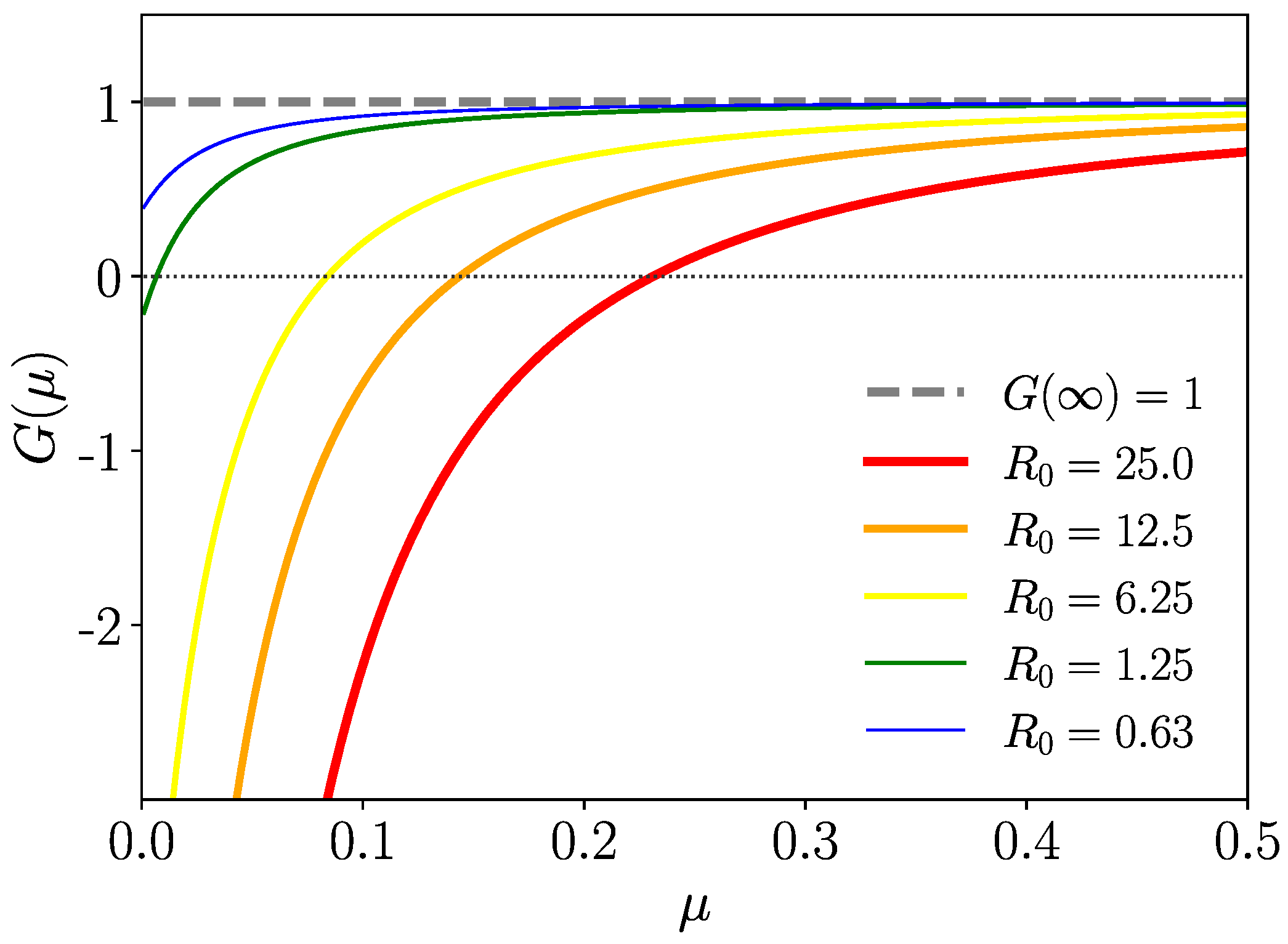
where is the basic reproduction number modified by mortality with (equality only for zero mortality). To visualize the effect of mortality on the instability of the healthy state, we plot for a few values of in Figure 5. Increasing mortality turns an unstable healthy state into a stable one.
In the random walk simulations, we deal with Gamma-distributed , where the persistence probabilities are then normalized incomplete Gamma functions (27). To explore the effect of mortality for such cases, we determine by numerical integration of (48) as a function of the mortality rate parameter and plot the result in Figure 6, where one can see that is monotonously decreasing with mortality rate . We also include a case of a fat-tailed (Mittag–Leffler)-distributed , which we discuss hereafter. The parameters in Figure 6 are such that the zero mortality case occurs with as the upper bound for the Gamma-distributed cases. The essential feature is that decays monotonically with increasing mortality rate parameter approaching zero for . Diseases with high mortality stabilize the healthy state even for .
Consider briefly the case where is exponentially distributed (i.e., in the Gamma distribution of ) with . Then, we have ; thus,
The zero mortality case is recovered for with . For Gamma-distributed , this yields
where , are the parameters of the respective Gamma distributions of the infection times of nodes and walkers. The Markovian case where all waiting times are exponentially distributed is covered for and yields
containing the zero mortality case for .
Fat-Tailed-Distributed
Finally, an interesting case emerges if follows a fat-tailed distribution, i.e., for t large () and , . Let us take a look at how mortality is affecting this situation. Fat-tailed distributions describe diseases where the infectious periods are very long and the healthy state without mortality is extremely unstable (). Infected walkers can infect many nodes during their long infection time spans. An important case of this class is constituted by the Mittag–Leffler (ML) distribution , where indicates the Mittag–Leffler function; see [33,34] and the references therein for representations and connections with fractional calculus. The ML function recovers the exponential for (). Assuming exponential mortality , one obtains with (51)
containing the LT of the ML persistence probability distribution . The essential feature here is that is weakly singular at with a monotonously decreasing scaling law, where the healthy state becomes stable for mortality parameters larger as . We depict this case in Figure 6 for (violet curve).
6. Random Walk Simulations
The remainder of our paper is devoted to testing the mean-field model under “real-world conditions”, which we mimic by random walkers navigating independently on an undirected connected (ergodic) graph. In our simulations, we focused on Barabási–Albert (BA), Erdös–Rényi (ER), and Watts–Strogatz (WS) graphs [16,17,35] (see Appendix A.4 for a brief recap) and implemented the compartments and transmission pathway for walkers and nodes outlined in Section 2. A susceptible walker gets infected with probability by visiting an infected node, and a susceptible node gets infected with probability at a visit of an infectious walker. We assumed that the infection probabilities are constant for all nodes and walkers, respectively. They are related, yet not identical to the macroscopic rate constants . A critical issue is whether the simple bi-linear forms for the mean-field infection rates (1) still capture the complexity of the spreading in such “real world” networks well. One goal of the subsequent case study is to explore this question.
We characterize the network topology by nodes with the adjacency matrix , where if the pair of nodes is connected by an edge and if the pair is disconnected. Further, we assumed to avoid self-connections of nodes. We confined ourselves to undirected networks, where the edges have no direction and the adjacency matrix is symmetric. The degree of a node i counts the number of neighbor nodes (edges) of this node. Each walker performs simultaneous independent random steps at discrete time instants from one to another connected node. The steps from a node i to one of the neighbor nodes are chosen with probability , following for all walkers the same transition matrix:
which is normalized . This is a common way to connect the network topology with simple Markovian random walks [30,35]. In the simulations, the departure nodes at of the walkers are randomly chosen. The path of each walker is independent and not affected by contacts with other walkers or by transition events from one to another compartment.
Case Study and Discussion
In order to compare the epidemic dynamics of the mean-field model and random walk simulations, we integrated the stochastic evolution Equation (2) numerically as follows. We averaged the increments of the compartmental fractions in a generalized Monte Carlo sense converging towards the convolutions of the right-hand side of (9), where we use the Monte Carlo convergence feature:
for random variables T drawn from PDFs . We performed this average for any time increment with respect to all involved independent random time spans (see Appendix A.1) and integrated the averaged compartmental increments in a fourth-order Runge–Kutta scheme (RK4). We used in the random walk simulations and the Monte Carlo (mean-field) integration exactly the same (Gamma-distributed) random values (Python 3.10.8 seeds) for . The values of the infection rate parameters used in the mean-field integration were determined from Equation (32) by plugging in the large time asymptotic values of the random walk simulation with identical parameters (without mortality). The compartmental fractions in the random walk simulations were determined by simply counting the compartmental populations at each time increment of the walker’s steps. The so-determined rate parameters plugged into the mean-field integration depend in a complex manner on the infection probabilities and topology of the network. In this way, this information is also contained in the basic reproduction numbers with and without mortality. Indeed, the importance of the structural features (topology) of the network is crucial for the spreading of the disease. We refer to the recent review article [36] exploring a large variety of these effects. In that work, a detailed study was performed on the role of structural elements such as the average distance of the nodes and the effective network size (among others) on the epidemic spreading. Naturally, pure mean-field (compartment) approaches ignore the topological features of the environments where the diseases are spreading. In our mean-field model, the structural network properties are captured by the infection rate parameters as outlined above.
We explore now the spreading in random graphs of different complexity such as represented in Figure 7. The BA graph is small-world with a power law-distributed degree (Appendix A.4), which means that there are many nodes having a few connections and a few (hub) nodes with a huge number of connections. The average distance between nodes becomes small, as it is sufficient that almost every node is only a few links away from a hub node. The ER graph is small-world due to a broad degree distribution. The WS graph with the choice of connectivity parameter in Figure 7 has long average distances and is large-world. Intuitively, one infers that a small-world structure is favorable for spreading processes, a feature that was already demonstrated in the literature [8,9]. In our simulations, spreading in network architectures with increased connectivity comes along with increased values of and , respectively.
We identified the starting time instant () of the evolution in the mean-field model with the time instant of the first infection of a walker in the random walk simulations. In all cases, we started with a small number of randomly chosen initially infected nodes () and no infected or dead walkers. To reduce the number of parameters and to concentrate on topological effects, we have put in all simulations the transmission probabilities . We refer to [37] for the Python codes (free to download and non-commercial use) and animated simulation videos related to the present study.
In order to visualize a typical spreading process, we depict in Figure 8 a few snapshots in a Watt–Strogatz graph with a rather high overall mortality probability of . In this case, a single infection wave emerges where a large part of the walkers gets repeatedly infected, increasing their probability to die. This leads to a very high fraction of eventually dead walkers and a small fraction of surviving walkers corresponding to the stationary state (17), which is taken as soon as the disease becomes extinct . Figure 8 shows that, first, the infection gains large parts of the network, consistent with the large value of observed in this case. After the first wave, the disease becomes extinct by the high mortality of the walkers. A disease with similar high mortality characteristics is, for instance, pestilence. The process of Figure 8 is visualized in an animated video https://drive.google.com/file/d/1-fhroAsoAVDKGR5H9yWtqjD7A1ZU5pQt/view (accessed on 22 April 2024).
Figure 9 and Figure 10 show the evolution in the WS graphs with identical parameters and Gamma distributions of as in Figure 8, but with a different mortality rate parameter and a much smaller overall mortality . The different network connectivity leads to different values of and mean-field solutions in Figure 9 and Figure 10. In addition, the networks of Figure 9 and Figure 10 have different connectivity features. The WS graph of Figure 9 is small-world (strongly connected), whereas the WS graph in Figure 10 is weakly connected and large-world. Comparing Figure 9 and Figure 10 shows that the network with higher connectivity of Figure 9 has higher values of or , respectively. The graph in Figure 9 is small-world with larger connectivity parameter coinciding with the average degree, i.e., has shorter average distances between nodes as the graph of Figure 10, which has connectivity parameter with clearly larger average distances between the nodes. The graph of Figure 9 with higher connectivity has (), whereas the graph of Figure 10 with lower connectivity has much smaller ( 107.92). Hence, the spreading (at ) in the graph with higher connectivity is much stronger as in the less well-connected structure. The effect of the smaller connectivity on the spreading can also be clearly seen by means of the delayed increase of the infection numbers produced by the random walk simulations (red curves) in Figure 10. One further observes in Figure 9 that the infection numbers exhibit strong and immediate increases followed by attenuated oscillations around the endemic equilibrium (for zero mortality) with high values and . The basic reproduction numbers with mortality are in both graphs only slightly smaller as . This is due to a rather small overall mortality of . This effect can also be seen in the small overlap of the Gamma distributions of and in the histogram. Recall that a small value of does not necessarily mean small since this quantity depends also on the infection rates and network topology (see (17)) and is sensitive to repeated infections, which may indeed play an important role here as is rather small.
In Figure 10, the infections of the random walk simulations are increasing more slowly (red curves) compared to Figure 9. The structure with higher connectivity in Figure 9 shows excellent quantitative agreement of the random walk and mean-field solutions for the walkers and nodes, well capturing the attenuated oscillations, especially for zero mortality. In the network with smaller connectivity of Figure 10, the increase of the infections is delayed compared to the mean field. On the other hand, for non-zero mortality, the mean-field and random walk dynamics for the walkers diverge slightly with time. We infer that mortality may deviate the infection rates from (1).
The comparison of the spreading in Figure 9 and Figure 10 shows clearly the role of the connectivity: the mean-field model better captures the spreading in networks with higher connectivity (short average distances between nodes) and with low mortality. The following cases give further evidence for these observations.
Next, we explore the spreading on an ER graph in Figure 11. The agreement of random walk simulations and the mean-field model is impressive, where this holds for both with and without mortality. One can see by means of the high average degree and the degree distribution in Figure 7 that, for these connectivity parameters, the graph is well-connected and small-world, giving strong evidence that the mean-field approach is here capturing the spreading dynamics well.
Finally, we explore in Figure 12 the dynamics on a BA network. In the right frame, we have high overall mortality of probability for a walker to die from an infection. In this example, the disease is starting to spread as , where only a single infection wave emerges, which is made extinct by the high mortality. Recall that is only telling us that the healthy state is unstable, i.e., that the disease is starting to spread. It does not contain the information about whether the spreading is persistent or whether the disease is eventually made extinct. To explore the role of topological features such as the average distances between nodes, we performed the same simulation experiment with identical parameters and less () nodes, i.e., a higher density of walkers (Figure 13).
The accordance of the mean-field model and random walk simulation is indeed also, as seen in Figure 13, excellent. We explain this by the fact that the BA network is a strongly connected structure with a pronounced small-world property. The higher density of walkers leads to increased and compared to Figure 12. There is also only a single infection wave occurring with a higher maximum value compared to Figure 12. In both cases (Figure 12 and Figure 13, right frames) the infection waves are made extinct by the high mortality of walkers, where stationary states (17) with of dead walkers are taken. When we switch off mortality (left frames), stable endemic states emerge more rapidly in Figure 13 (the case with a higher density of walkers).
Further simulation experiments (not shown here) revealed that the mean-field model and random walk simulations exhibited excellent accordance when we further increased the attachment parameters m or the density of walkers with otherwise identical parameters. For higher mortality, the agreement becomes less good and diverges with increasing observation time. This observation suggests that mortality modifies the infection rates in the network for larger observation times. We leave this issue for future research.
Our overall finding from this case study is that the mean-field approach (with infection rates (1)) is particularly well suited to mimic spreading in strongly connected environments with a pronounced small-world feature, but is less good for higher mortality.
7. Conclusions
We studied epidemic spreading in complex graphs, where we focused on the transmission pathway via vectors mimicking the spreading of a certain class of diseases such as Dengue, Malaria, Pestilence, and others. We developed a stochastic compartment model for the walkers and nodes with mortality for the walkers. For zero mortality, we obtained the endemic equilibrium in explicit form (Equation (33)). The stability analysis of the endemic and healthy states revealed the crucial control parameter for spreading, the basic reproduction number. We obtained the basic reproduction numbers and with and without mortality, respectively, where we proved that (the relations (50) with (48)). For , the healthy state is an unstable fixed point where the endemic equilibrium exists for zero mortality as a unique stable fixed point independent of the initial conditions. The basic reproduction numbers depend on the means of the compartmental sojourn times in compartment I of the nodes and walkers and on the topology of the network captured by the mean-field rate constants . For future research, it would be desirable to extend the mean-field model in such a way that it connects the rate parameters in explicit form with the topological features of the network such as the mean distance of the nodes, average connectivity, and others. We refer to [38] for a recent study connecting the spreading of COVID-19 with such topological features, where it has to be emphasized that COVID-19 is not a vector-transmitted disease and, hence, does not refer to the class of diseases analyzed here.
Our model has applications beyond epidemic dynamics, for instance in chemical reaction models [39], and can be extended in various directions. For instance, the inclusion of additional compartments and natural birth and death processes based on real-world observations of Malaria transmission dynamics is of interest [40]. An interesting question to explore in a follow-up project is whether our class of compartment models with indirect transmission pathways may exhibit (for zero mortality) persistent oscillations (Hopf instabilities). (See our brief discussion at the end of Appendix A.2.) An open problem also remains how a large-world network topology may be included in such a mean-field model, modifying the infection rates. Further promising directions include an accounting of immune and incubation compartments, the effects of mitigation measures, and vaccinations, among many others.
Author Contributions
Conceptualization, T.M.M. and M.B.; Methodology, T.G., T.M.M. and A.P.R.; Validation, T.G., T.M.M., A.P.R. and B.A.C.; Formal analysis, T.G., T.M.M., M.B. and A.P.R.; Investigation, T.G., T.M.M., M.B., A.P.R. and B.A.C.; Writing—original draft, T.M.M.; Writing—review & editing, T.G., M.B. and A.P.R.; Project administration, B.A.C. All authors have read and agreed to the published version of the manuscript.
Funding
This research received no external funding.
Data Availability Statement
No new data were created or analyzed in this study. Data sharing is not applicable to this article.
Acknowledgments
T.G. gratefully acknowledges to have been hosted at the Institut Jean le Rond d’Alembert in the framework of an internship (stage M1 Physique ) for the development of the Python simulation codes and participation in the present study.
Conflicts of Interest
The authors declare no conflict of interest.
Appendix A
Appendix A.1. Some Basic Notions
Here, we recall briefly some basic notions used in the paper. The infection rates are causal functions:
where indicates the Heaviside step function defined by
with , and in our definition, . Its derivative yields the Dirac -distribution . We use throughout the paper mutually independent strictly positive random variables The random variables are assumed to follow their specific PDFs:
where the PDFs are causal functions as a consequence of the positiveness of the . Then, the averaging rule applies:
for suitable functions f. For , using the independence of the , this yields
Important cases emerge by applying (A4) to the exponentials:
In this relation, the LTs of the PDFs come into play:
where reflects the normalization of PDFs (A3). A further observation is
where ★ stands for the convolution of the causal PDFs.
Appendix A.2. Proof of Stability of the Endemic Equilibrium
Here, we develop the rest of the proof of the stability of the endemic equilibrium, i.e., we show that the function (42) is strictly positive for with . First, we observe that with and . For our convenience, we introduce the functions
which are the LTs of the normalized functions and which are, by virtue of Bernstein’s theorem [41], completely monotonic (CM) with respect to , i.e.,
inheriting this feature from the exponential (). Therefore,
(as ) exists; thus, is monotonously decreasing with with . Further, we observe in Equation (33) that , ; thus,
Then, reads
Now, we observe that ; thus, a lower bound function is generated by replacing in the second line. Now, it is sufficient to prove that . We, hence, obtain for this lower bound function:
and with and , it follows that , concluding the proof of the stability of the endemic equilibrium.
Appendix A.3. A Few Remarks on the Possibility of Oscillatory (Hopf) Instabilities of the Endemic Equilibrium
Let us briefly explore whether an oscillatory (Hopf) instability of the endemic equilibrium is possible. To that end, we write as
where and is a non-negative CM function (see Figure 4) with the maximum value . Then, the following two cases may occur.
Case (i) ; ():
Then, can be represented as the LT of a non-negative function , and consider, now, with ; thus, the real part of can be written as
with and, clearly, . Therefore,
Hence, in the range of case (i) , there is no oscillatory (Hopf) instability of the endemic state possible (a similar consideration of function of (39) shows as well that the healthy state for does not exhibit an oscillatory instability):
Case (ii) ; :
Here, we have two pertinent ranges of . The first is the range (a) (i.e., ), and the second one (b) is . Clearly, in the range (a), (A14) remains true and strictly positive. Hence, for , no Hopf instability is possible.
This changes in the range (b), since ; thus, may become negative. Therefore, for , a Hopf instability of the endemic state becomes possible. However, the possibility that is only necessary, but not sufficient for a Hopf instability. One also needs simultaneously that the imaginary part is vanishing for the same . In the simulations performed for this paper, we did not observe persistent oscillations. We leave the exploration of this issue for future research in a follow-up project.
Appendix A.4. A Very Brief Recap of Random Graphs
Here, we recall briefly some essential features of the three classes of random graphs, which we use in the random walk simulations. For an extended outline, consult, e.g., [42]. The three classes of random graph models depicted hereafter are motivated by the observation that complex random network structures are encountered ubiquitously and crucially determine human and animal mobility patterns, including epidemic propagation.
- (i)
- Erdös and Rényi (ER) graph
The ER graph is one of the most basic variants of a random graph, which was introduced in 1959 by Erdös and Rényi [43]. We use the so-called variant of the random ER graph model, which is actually due to Gilbert [44], and generated as follows [11,14]. Given are N labeled nodes. Any pair of nodes is connected independently by an edge with uniform probability p. The probability that a node has connections is given by a binomial distribution:
where denotes the average degree. For (while is kept constant), the degree distribution converges to a Poisson distribution representing the infinite graph limit of the ER model. Therefore, is rapidly decaying with degree k, so the number of nodes with a high number of connections is very small. In order to obtain in the model a connected graph, it is necessary that be above the percolation limit [30,43]:
- (ii)
- Watts–Strogatz (WS) network:
The WS graph model [11,45,46] starts with a ring of N nodes, where each node is connected symmetrically with a number to the left and right neighbor nodes by an edge such that each node has connections. In the second step, each of the connections of node i is replaced with probability p by a randomly chosen connection uniformly among other nodes avoiding self-connections and link duplication, so that each connection is chosen only once. There are two noteworthy limits for a WS graph. For (no rewiring of links), we have a regular ring with constant degree for all nodes. In the limit , an ER graph is emerging with probability for a link. The WS graph has the small-world property (short average distances between pairs of nodes) and a high tendency to develop clusters of nodes [46].
- (iii)
- Barabási–Albert (BA) graph:
The BA graph is generated by a preferential attachment mechanism for newly added nodes [14,15,42,47]. One starts with nodes and adds new nodes. Any newly added node is connected with existing nodes (m is referred to as the attachment parameter), most likely with nodes of high degrees. In this way, nodes with a high degree receive further links. This leads to an asymptotically scale-free network with a power law degree distribution:
As the decrease in this power law is relatively slow, there might exist quite a few nodes with many links (hub nodes) and many nodes with few links. BA graphs are believed to mimic a large class of real-world networks including the World Wide Web and citation, social, and metabolic networks.
Realizations of these three types of random graphs are used in our multiple random walker simulations and shown in Figure 7.
References
- Rhodes, P.; Bryant, J.H. Public Health. Encyclopedia Britannica. 2024. Available online: https://www.britannica.com/topic/public-health (accessed on 22 April 2024).
- Kermack, W.O.; McKendrick, A.G. A contribution to the mathematical theory of epidemics. Proc. Roy. Soc. A 1927, 115, 700–721. [Google Scholar]
- Liu, W.M.; Hethcote, H.W.; Levin, S.A. Dynamical behavior of epidemiological models with non-linear incidence rate. J. Math. Biol. 1987, 25, 359–380. [Google Scholar] [CrossRef]
- Li, M.Y.; Graef, J.R.; Wang, L.; Karsai, J. Global dynamics of a SEIR model with varying total population size. Math. Biosci. 1999, 160, 191–213. [Google Scholar] [CrossRef] [PubMed]
- Anderson, R.M.; May, R.M. Infectious Diseases in Humans; Oxford University Press: Oxford, UK, 1992. [Google Scholar]
- Martcheva, M. An Introduction to Mathematical Epidemiology; Springer: Berlin/Heidelberg, Germany, 2015. [Google Scholar]
- Harris, J.E. Population-Based Model of the Fraction of Incidental COVID-19 Hospitalizations during the Omicron BA.1 Wave in the United States. COVID 2023, 3, 728–743. [Google Scholar] [CrossRef]
- Pastor-Satorras, R.; Castellano, C.; Mieghem, P.V.; Vespignani, A. Epidemic processes in complex networks. Rev. Mod. Phys. 2015, 87, 925–979. [Google Scholar] [CrossRef]
- Pastor-Satorras, R.; Vespignani, A. Epidemic dynamics and endemic states in complex networks. Phys. Rev. E 2001, 63, 066117. [Google Scholar] [CrossRef]
- Okabe, Y.; Shudo, A. Microscopic Numerical Simulations of Epidemic Models on Networks. Mathematics 2021, 9, 932. [Google Scholar] [CrossRef]
- Newman, M.E.J.; Watts, D.J.; Strogatz, S.H. Random graph models of social networks. Proc. Natl. Acad. Sci. USA 2002, 99, 2566–2572. [Google Scholar] [CrossRef]
- Eraso-Hernandez, L.K.; Riascos, A.P.; Michelitsch, T.M.; Wang-Michelitsch, J. Evolution of transport under cumulative damage in metro systems. Int. J. Mod. Phys. C 2023, 35, 2450037. [Google Scholar] [CrossRef]
- Barrat, A.; Barthélemy, M.; Vespignani, A. Epidemic spreading in population networks. In Dynamic Processes on Complex Networks; Cambridge University Press: Cambridge, UK, 2008; pp. 180–215. [Google Scholar] [CrossRef]
- Barabási, A.-L. Network Science; Cambridge University Press: Cambridge, UK, 2016. [Google Scholar]
- Barabási, A.-L.; Albert, R. Emergence of Scaling in Random Networks. Science 1999, 286, 509. [Google Scholar] [CrossRef]
- Riascos, A.P.; Sanders, D.P. Mean encounter times for multiple random walkers on networks. Phys. Rev. E 2021, 103, 042312. [Google Scholar] [CrossRef] [PubMed]
- Michelitsch, T.M.; Riascos, A.P.; Collet, B.A.; Nowakowski, A.F.; Nicolleau, F.C.G.A. Fractional Dynamics on Networks and Lattices; ISTE/Wiley: London, UK, 2019. [Google Scholar]
- van Kampen, N.G. Stochastic Processes in Chemistry and Physics; North Holland: Amsterdam, The Netherlands, 1981. [Google Scholar]
- Ross, S.M. Stochastic Processes; John Wiley & Sons: New York, NY, USA, 1996. [Google Scholar]
- Van Mieghem, P. Exact Markovian SIR and SIS epidemics on networks and an upper bound for the epidemic threshold. arXiv 2014, arXiv:1402.1731. [Google Scholar]
- Bestehorn, M.; Riascos, A.P.; Michelitsch, T.M.; Collet, B.A. A Markovian random walk model of epidemic spreading. Contin. Mech. Thermodyn. 2021, 33, 1207–1221. [Google Scholar] [CrossRef] [PubMed]
- Bestehorn, M.; Michelitsch, T.M. Oscillating Behavior of a Compartmental Model with Retarded Noisy Dynamic Infection Rate. Int. Bifurc. Chaos 2023, 33, 2350056. [Google Scholar] [CrossRef]
- Bestehorn, M.; Michelitsch, T.M.; Collet, B.A.; Riascos, A.P.; Nowakowski, A.F. Simple model of epidemic dynamics with memory effects. Phys. Rev. E 2022, 105, 024205. [Google Scholar] [CrossRef] [PubMed]
- Granger, T.; Michelitsch, T.M.; Bestehorn, M.; Riascos, A.P.; Collet, B.A. Four-compartment epidemic model with retarded transition rates. Phys. Rev. E 2023, 107, 044207. [Google Scholar] [CrossRef] [PubMed]
- Basnarkov, L.; Tomovski, I.; Sandev, T.; Kocarev, L. Non-Markovian SIR epidemic spreading model of COVID-19. Chaos Solitons Fractals 2022, 160, 112286. [Google Scholar] [CrossRef] [PubMed]
- Zhu, Y.; Shen, R.; Dong, H.; Wang, W. Spatial heterogeneity and infection patterns on epidemic transmission disclosed by a combined contact-dependent dynamics and compartmental model. PLoS ONE 2023, 18, e0286558. [Google Scholar] [CrossRef] [PubMed]
- Gostiaux, L.; Bos, W.J.T.; Bertoglio, J.-P. Periodic epidemic outbursts explained by local saturation of clusters. Phys. Rev. E 2023, 107, L012201. [Google Scholar] [CrossRef]
- Peyrard, M. What can we learn from the dynamics of the COVID-19 epidemic? Chaos 2023, 33, 103101. [Google Scholar] [CrossRef]
- Soper, H.E. The interpretation of periodicity in disease prevalence. J. R. Stat. Soc. 1929, 92, 34–61. [Google Scholar] [CrossRef]
- Newman, M.E.J. Networks: An Introduction; Oxford University Press: Oxford, UK, 2010. [Google Scholar]
- Whitehead, S.S.; Blaney, J.E.; Durbin, A.P.; Murphy, B.R. Prospects for a dengue virus vaccine. Nat. Rev. Microbiol. 2007, 5, 518–528. [Google Scholar] [CrossRef] [PubMed]
- d’Onofrio, G.; Michelitsch, T.M.; Polito, F.; Riascos, A.P. On discrete-time arrival processes and related random motions. arXiv 2024, arXiv:2403.06821. [Google Scholar]
- Metzler, R.; Klafter, J. The random walk’s guide to anomalous diffusion: A fractional dynamics approach. Phys. Rep. 2000, 339, 1–77. [Google Scholar] [CrossRef]
- Mainardi, F.; Gorenflo, R.; Scalas, E. A fractional generalization of the Poisson processes. Vietnam J. Math. 2004, 32, 53–64. [Google Scholar]
- Noh, J.-D.; Rieger, H. Random walks on complex networks. Phys. Rev. Lett. 2004, 92, 11. [Google Scholar] [CrossRef] [PubMed]
- Bellingeri, M.; Bevacqua, D.; Scotognella, F.; Cassi, D. The Critical Role of Networks to Describe Disease Spreading Dynamics in Social Systems: A Perspective. Mathematics 2024, 12, 792. [Google Scholar] [CrossRef]
- Supplementary Materials: Python Codes (© Téo Granger 2023) and Animated Films. Available online: https://sites.google.com/view/scirs-model-supplementaries/accueil (accessed on 22 April 2024).
- Thurner, S.; Klimek, P.; Hanel, R. A network-based explanation of why most COVID-19 infection curves are linear. Proc. Natl. Acad. Sci. USA 2020, 117, 22684–22689. Available online: https://www.pnas.org/doi/epdf/10.1073/pnas.2010398117 (accessed on 22 April 2024). [CrossRef]
- Simon, C.M. The SIR dynamic model of infectious disease transmission and its analogy with chemical kinetics. PeerJ Phys. Chem. 2020, 2, e14. [Google Scholar] [CrossRef]
- Ochieng, F.O. SEIRS model for malaria transmission dynamics incorporating seasonality and awareness campaign. Infect. Dis. Model 2024, 9, 84–102. [Google Scholar] [CrossRef]
- Schilling, R.; Song, R.; Vondraček, Z. Bernstein Functions; Theory and Applications, Studies in Mathematics, 37; De Gruyter: Berlin, Germany, 2010. [Google Scholar]
- Albert, B.R.; Jeong, H. Mean-field theory for scale-free random networks. Physical A 1999, 272, 173–187. [Google Scholar]
- Erdös, P.; Rényi, A. On Random Graphs I. Publ. Math. 1959, 6, 290–297. [Google Scholar] [CrossRef]
- Gilbert, E.N. Random Graphs. Ann. Math. Sci. 1959, 30, 1141–1144. [Google Scholar] [CrossRef]
- Erdös, P.; Rényi, P. On the evolution of random graphs. Publ. Math. Inst. Hung. Acad. Sci. 1960, 5, 17. [Google Scholar]
- Watts, D.J.; Strogatz, S.H. Collective dynamics of ‘small-world’ networks. Nature 1998, 393, 440. [Google Scholar] [CrossRef]
- Jeong, H.; Tombor, B.; Albert, R.; Oltvai, Z.N.; Barabási, A.L. The large-scale organization of metabolic networks. Nature 2000, 407, 651–654. [Google Scholar] [CrossRef]
Figure 1.
Left frame: Gamma distribution for four different cases: weakly singular (at ) [, ], exponential [, ], broad [, ], and narrow [, ]. Right frame: Their persistence (survival) probability distributions of Equation (27), where the same color code is used.
Figure 1.
Left frame: Gamma distribution for four different cases: weakly singular (at ) [, ], exponential [, ], broad [, ], and narrow [, ]. Right frame: Their persistence (survival) probability distributions of Equation (27), where the same color code is used.

Figure 2.
Endemic states of infected walkers/nodes versus for various values of parameter r, which has to be read () for the walker’s (node’s) endemic states.
Figure 2.
Endemic states of infected walkers/nodes versus for various values of parameter r, which has to be read () for the walker’s (node’s) endemic states.

Figure 3.
of (39) for some Gamma-distributed . Positive zeros of exist only for (instability of globally healthy state).
Figure 3.
of (39) for some Gamma-distributed . Positive zeros of exist only for (instability of globally healthy state).

Figure 4.
of (42) for different values of , where for (stability of the endemic state).
Figure 4.
of (42) for different values of , where for (stability of the endemic state).

Figure 5.
We depict function of Equation (47) for a few values of for exponentially distributed . The basic reproduction number is monotonously decreasing with increasing mortality parameter (see Figure 6). The parameters are , , , , with , where, here, .

Figure 6.
Basic reproduction number of Equation (52) versus mortality rate parameter for Gamma-distributed for various , where we have set , () and , for the Markovian case, which is recovered by Equation (53).

Figure 7.
Barabási–Albert, Erdös–Rényi, and Watts–Strogatz types with 300 nodes and connectivity parameters used in some of the simulations. The WS graph for connectivity parameter lacks the small-world property, resembling a complex real-world structure. The ER network has a broad degree distribution and the small-world property. The BA graph is for asymptotically scale-free with a power law degree distribution and the small-world feature, where a large number of nodes have small degrees and, a few (hub) nodes, very large degrees. Almost all nodes are only a few links away from hub nodes.

Figure 8.
Snapshots of spreading in a WS graph ( walkers, nodes, connectivity parameter ) and mortality parameter with . The average degree is , here coinciding with connectivity parameter m. Other parameters are the same as in Figure 9. The upper frames show the evolution from the random walk data. One observes and with only about 20 surviving walkers after extinction of the disease. S walkers are drawn in cyan color; I walkers are in red; D walkers are invisible; nodes without walkers are represented in black. Consult here an animated video of this process https://drive.google.com/file/d/1-fhroAsoAVDKGR5H9yWtqjD7A1ZU5pQt/view (accessed on 22 April 2024).

Figure 9.
The plots show the evolution on the WS graph with walkers for connectivity parameter (coinciding with the average degree) and rewiring probability () without mortality (left frame) and with mortality (right frame). are Gamma-distributed with the parameters , , , , and , ; see the histogram. The overall mortality is the same as in Fig. Figure 10 and determined by the numerical integration of (7). The random walk data are generated by averaging over 50 random walk realizations.

Figure 10.
Evolution on the WS graph with walkers and nodes for the same parameters as in Figure 9 averaged over 50 random walk realizations, but with reduced connectivity parameter . The upper frame shows a snapshot () of the spreading in one random walk realization (susceptible walkers green, susceptible nodes black, infected nodes red).

Figure 11.
Evolution on the ER graph () with walkers and small probability (above the percolation limit to ensure a connected structure). The parameters are , , , , , . The average degree of this ER graph is very large with .
Figure 11.
Evolution on the ER graph () with walkers and small probability (above the percolation limit to ensure a connected structure). The parameters are , , , , , . The average degree of this ER graph is very large with .

Figure 12.
Evolution on Barabási–Albert graph with walkers and nodes ( and the average degree ) with parameters , , , (sharp ), , . The basic reproduction number is here only slightly smaller than without mortality. The left upper frame shows the initial condition. S walkers are represented in blue, I walkers in red, and nodes in black. The random walk data are generated by averaging over 10 random walk realizations.

Figure 13.
Evolution with the same parameters and number of walkers () as in Figure 12, but fewer nodes () for one random walk realization and average degree . We interpret the increase of and due to more frequent passages of susceptible walkers on infected nodes (higher infection rates). Here, we performed only one random walk realization.

Disclaimer/Publisher’s Note: The statements, opinions and data contained in all publications are solely those of the individual author(s) and contributor(s) and not of MDPI and/or the editor(s). MDPI and/or the editor(s) disclaim responsibility for any injury to people or property resulting from any ideas, methods, instructions or products referred to in the content. |
© 2024 by the authors. Licensee MDPI, Basel, Switzerland. This article is an open access article distributed under the terms and conditions of the Creative Commons Attribution (CC BY) license (https://creativecommons.org/licenses/by/4.0/).
Share and Cite
MDPI and ACS Style
Granger, T.; Michelitsch, T.M.; Bestehorn, M.; Riascos, A.P.; Collet, B.A. Stochastic Compartment Model with Mortality and Its Application to Epidemic Spreading in Complex Networks. Entropy 2024, 26, 362. https://doi.org/10.3390/e26050362
AMA Style
Granger T, Michelitsch TM, Bestehorn M, Riascos AP, Collet BA. Stochastic Compartment Model with Mortality and Its Application to Epidemic Spreading in Complex Networks. Entropy. 2024; 26(5):362. https://doi.org/10.3390/e26050362
Chicago/Turabian StyleGranger, Téo, Thomas M. Michelitsch, Michael Bestehorn, Alejandro P. Riascos, and Bernard A. Collet. 2024. "Stochastic Compartment Model with Mortality and Its Application to Epidemic Spreading in Complex Networks" Entropy 26, no. 5: 362. https://doi.org/10.3390/e26050362
Note that from the first issue of 2016, this journal uses article numbers instead of page numbers. See further details here.