On the Linear Combination of Exponential and Gamma Random Variables
1
Department of Statistics, University of Nebraska, Lincoln, NE 68583, USA
2
Department of Engineering Management and Systems Engineering, The George Washington University, Washington, D.C. 20052, USA
Entropy 2005, 7(2), 161-171; https://doi.org/10.3390/e7020161
Submission received: 27 January 2005
/
Accepted: 13 June 2005
/
Published: 14 June 2005
Abstract
:The exact distribution of the linear combination αX + βY is derived when X and Y are exponential and gamma random variables distributed independently of each other. A measure of entropy of the linear combination is investigated. We also provide computer programs for generating tabulations of the percentage points associated with the linear combination. The work is motivated by examples in automation, control, fuzzy sets, neurocomputing and other areas of computer science.
Keywords:
entropy; exponential distribution; gamma distribution; linear combinations of random variablesMSC 2000 codes:
33C90, 62E991 Introduction
For given random variables X and Y , the distribution of linear combinations of the form αX + βY is of interest in problems in automation, control, fuzzy sets, neurocomputing and other areas of computer science. Some examples are:
- In automatic control, one often encounters the problem of maximizing the expected sum of n variables, chosen from a sequence of N sequentially arriving i.i.d. scalar random variables, X1, X2, . . . , XN. The objective is to devise a decision rule so as to maximize , where ki ∈ {1, 2, . . . , N} is the index of the ith random variable selected. At time k, the random variable Xk is observed, and the decision to select the value or not must be taken online. This problem is known as the sequential screening problem and many decision problems can be formulated in this way (Pronzato [1]).
- The theory of congruence equations (see, for example, Cerruti [2]) has applications in computer science. There is a wide literature about congruence equations and the last twenty years has seen interesting formulas and functions derived: among these, expressions giving the number of solutions of linear congruences. Counting such solutions has relations with statistical problems like the distribution of the values taken by particular sums.
- In neurocomputing, linear combinations are used for combining multiple probabilistic classifiers on different feature sets. In order to achieve the improved classification performance, a generalized finite mixture model is proposed as a linear combination scheme and implemented based on radial basis function networks. In the linear combination scheme, soft competition on different feature sets is adopted as an automatic feature rank mechanism so that different feature sets can be always simultaneously used in an optimal way to determine linear combination weights (Chen and Chi [3]).
The distribution of αX + βY has been studied by several authors especially when X and Y are independent random variables and come from the same family. For instance, see Fisher [10] and Chapman [11] for Student’s t family, Christopeit and Helmes [12] for normal family, Davies [13] and Farebrother [14] for chi-squared family, Ali [15] for exponential family, Moschopoulos [16] and Provost [17] for gamma family, Dobson et al [18] for Poisson family, Pham-Gia and Turkkan [19] and Pham and Turkkan [20] for beta family, Kamgar-Parsi et al [21] and Albert [22] for uniform family, Hitezenko [23] and Hu and Lin [24] for Rayleigh family, and Witkovský [25] for inverted gamma family.
However, there is relatively little work of the above kind when X and Y belong to different families. In the applications mentioned above, it is quite possible that X and Y could arise from different but similar distributions. In this paper, we study the exact distribution of αX + βY when X and Y are independent random variables having the exponential and gamma distributions with pdfs
and
respectively, for x > 0, y > 0, λ > 0, µ > 0 and a > 0. We assume without loss of generality that α > 0.
The paper is organized as follows. In Section 2, we derive explicit expressions for the pdf and the cdf of αX + βY. A measure of entropy of the linear combination is investigated in Section 3. In Section 4, we provide computer programs for generating tabulations of the percentage points associated with the linear combination. We hope that these programs will be of use to the practitioners mentioned above.
The calculations of this paper involve several special functions, including the incomplete gamma function defined by
the complementary incomplete gamma function defined by
and the error function defined by
The properties of the above special functions can be found in Prudnikov et al. [26] and Gradshteyn and Ryzhik [27].
2 PDF and CDF
Theorem 1 derives explicit expressions for the pdf and the cdf of αX + βY in terms of the incomplete gamma functions.
Theorem 1
Suppose X and Y are distributed according to (1) and (2), respectively. The cdf of Z = αX + βY can be expressed as
for β > 0 and z > 0, as
for β < 0 and z < 0, and as
for β < 0 and z ≥ 0. The corresponding pdfs are:
for β > 0 and z > 0,
for β < 0 and z < 0, and
for β < 0 and z ≥ 0.
Proof:
If β > 0 then the result follows by writing
where the last step follows from the definition of the incomplete gamma function. The result in (4) can be established similarly by using the definition of the complementary incomplete gamma function. The result in (5) follows by setting z = 0 into to the two incomplete gamma function terms in (4). ■
The following corollaries provide the cdfs for the sum and the difference of the exponential and gamma random variables.
Corollary 1
Suppose X and Y are distributed according to (1) and (2), respectively. Then, the cdf of Z = X + Y can be expressed as
for z > 0.
Corollary 2
Suppose X and Y are distributed according to (1) and (2), respectively. Then, the cdf of Z = X − Y can be expressed as
for z < 0 and as
for z ≥ 0.
Using special properties of the incomplete gamma functions, one can obtain simpler expressions for (3)–(4) when a takes integer or half integer values. This is illustrated in the corollaries below.
Corollary 3
If a ≥ 1 is an integer then (3)–(4) can be reduced to the simpler forms
for β > 0 and z > 0, and
for β < 0 and z < 0, where x = z(µα − λβ)/(αβ) and y = µz/β.
Corollary 4
Figure 1 below illustrates possible shapes of the pdfs (6)–(8) for selected values of α, β and a. The four curves in each plot correspond to selected values of a. As expected, the densities are unimodal and the effect of the parameters is evident.If a − 1/2 ≥ 0 is an integer then (3)–(4) can be reduced to the simpler forms
![Entropy 07 00161 i001]() for β > 0 and z > 0, and
for β > 0 and z > 0, and
![Entropy 07 00161 i002]() for β < 0 and z < 0, where x = z(µα − λβ)/(αβ) and y = µz/β.
for β < 0 and z < 0, where x = z(µα − λβ)/(αβ) and y = µz/β.


3 Entropy
An entropy of a random variable is a measure of variation of the uncertainty. The simplest known entropy is the Shannon entropy (Shannon [28]) defined by
Consider calculating this when Z has the pdfs described in Theorem 1. If β > 0 then one can write where I denotes the integral
where I denotes the integral
Unfortunately, this integral I cannot be reduced to a closed form even in the simplest case a = 1. Thus, one cannot obtain a closed form expression even for the simplest entropy measure when Z is distributed as in Theorem 1. Hence, we performed a numerical study to examine the behavior of (9) with respect to the parameters in Theorem 1. A program in R (Ihaka and Gentleman [29]) written to compute (9) is presented below.
cc<-lambda*((mu*alpha)**a)/(alpha*gamma(a)*(mu*alpha-lambda*beta)**a)
ff<-function (x)
{tt<-gamma(a)*pgamma(x*(mu*alpha-lambda*beta)/(alpha*beta),shape=a)
tt<-exp(-lambda*x/alpha)*tt*log(tt)
return(tt)}
ent<-1+lambda*beta*a/(alpha*mu)-log(cc)
ent<-ent-cc*integrate(ff,lower=0,upper=Inf)$value
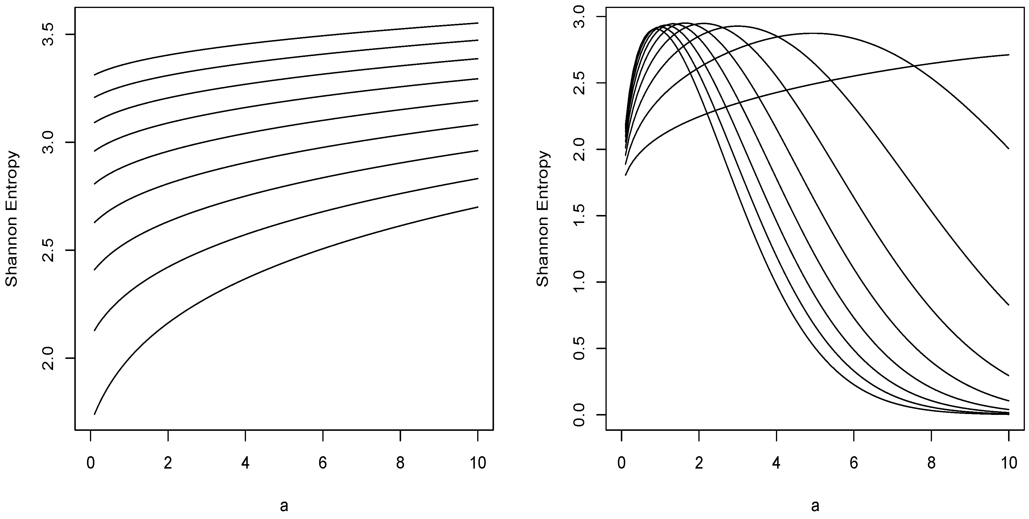
Figure 2 below shows the variation of (9) for a range of values of α, β and a with λ = 1 and µ = 1. The effect of the parameters is evident: for fixed β, (9) is an increasing function of both α and a; for fixed α, (9) increases with respect to β but, with respect to a, it initially increases before decreasing.
One could also consider other more advanced measures of entropy such as the Rényi entropy defined by
where γ > 0 and γ ≠ 1 (Rényi [30]). But, for the reasons mentioned above, one cannot obtain closed form expressions for these and the investigation will have to be performed numerically.
4 Percentiles
In this section, we provide two computer programs for generating tabulations of percentage points zp associated with the cdf of Z = αX + βY. These percentiles are computed numerically by solving the equations
and
Evidently, this involves computation of the incomplete gamma and the complementary incomplete gamma functions and routines for this are widely available. We used the function GAMMA (·) in the algebraic manipulation package, MAPLE. The MAPLE programs below compute the percentiles zp for p = 0.01, 0.05, 0.1, 0.90, 0.95, 0.99 for given values of α, β, λ, µ and a.
#this  program  gives  percentiles  when  beta  >  0
ff:=(1/GAMMA(a))*((mu*alpha)/(mu*alpha-lambda*beta))**a*exp(-lambda*z/alpha):
ff:=ff*(GAMMA(a)-GAMMA(a,z*(mu*alpha-lambda*beta)/(alpha*beta))):
ff:=1-GAMMA(a,mu*z/beta)/GAMMA(a)-ff:
p1:=fsolve(ff=0.01,z=0..1000):
p2:=fsolve(ff=0.05,z=0..1000):
p3:=fsolve(ff=0.1,z=0..1000):
p4:=fsolve(ff=0.90,z=0..1000):
p5:=fsolve(ff=0.95,z=0..1000):
p6:=fsolve(ff=0.99,z=0..1000):
print(p1,p2,p3,p4,p5,p6);

#this  program  gives  percentiles  when  beta  <  0
ff1:=(1/GAMMA(a))*((mu*alpha)/(mu*alpha-lambda*beta))**a:
ff1:=ff1*exp(-lambda*z/alpha):
ff1:=ff1*GAMMA(a,z*(mu*alpha-lambda*beta)/(alpha*beta)):
ff1:=GAMMA(a,mu*z/beta)/GAMMA(a)-ff1:
ff2:=1-((mu*alpha)/(mu*alpha-lambda*beta))**a*exp(-lambda*z/alpha):
bd:=1-((mu*alpha)/(mu*alpha-lambda*beta))**a:
if (bd>0.01) then p1:=fsolve(ff1=0.01,z=-1000..0): end if:
if (bd<=0.01) then p1:=fsolve(ff2=0.01,z=0..1000): end if:
if (bd>0.05) then p2:=fsolve(ff1=0.05,z=-1000..0): end if:
if (bd<=0.05) then p2:=fsolve(ff2=0.05,z=0..1000): end if:
if (bd>0.1) then p3:=fsolve(ff1=0.1,z=-1000..0): end if:
if (bd<=0.1) then p3:=fsolve(ff2=0.1,z=0..1000): end if:
if (bd>0.9) then p4:=fsolve(ff1=0.9,z=-1000..0): end if:
if (bd<=0.9) then p4:=fsolve(ff2=0.9,z=0..1000): end if:
if (bd>0.95) then p5:=fsolve(ff1=0.95,z=-1000..0): end if:
if (bd<=0.95) then p5:=fsolve(ff2=0.95,z=0..1000): end if:
if (bd>0.99) then p6:=fsolve(ff1=0.99,z=-1000..0): end if:
if (bd<=0.99) then p6:=fsolve(ff2=0.99,z=0..1000): end if:
print(p1,p2,p3,p4,p5,p6);
We hope these programs will be of use to the practitioners of the linear combination (see Section 1).
Acknowledgments
The authors would like to thank the referees and the editor for carefully reading the paper and for their great help in improving the paper.
References
- Pronzato, L. Optimal and asymptotically optimal decision rules for sequential screening and resource allocation. Transactions on Automatic Control 2001, 46, 687–697. [Google Scholar] [CrossRef]
- Cerruti, U. Counting the number of solutions of congruences. In Application of Fibonacci Numbers; Bergum, G. E., et al., Eds.; Kluwer Academic Publishers: Dordrecht, The Netherlands, 1993; vol 5, pp. 85–101. [Google Scholar]
- Chen, K.; Chi, H. A method of combining multiple probabilistic classifiers through soft competition on different feature sets. Neurocomputing 1988, 20, 227–252. [Google Scholar] [CrossRef]
- Boswell, S. B.; Taylor, M. S. A central limit theorem for fuzzy random variables. Fuzzy Sets and Systems 1987, 24, 331–344. [Google Scholar] [CrossRef]
- Williamson, R. C. The law of large numbers for fuzzy variables under a general triangular norm extension principle. Fuzzy Sets and Systems 1991, 41, 55–81. [Google Scholar] [CrossRef]
- Inoue, H. Randomly weighted sums for exchangeable fuzzy random variables. Fuzzy Sets and Systems 1995, 69, 347–354. [Google Scholar] [CrossRef]
- Jang, L. -C.; Kwon, J. -S. A uniform strong law of large numbers for partial sum processes of fuzzy random variables indexed by sets. Fuzzy Sets and Systems 1998, 99, 97–103. [Google Scholar] [CrossRef]
- Feng, Y. Sums of independent fuzzy random variables. Fuzzy Sets and Systems 2001, 123, 2011. 11–18. [Google Scholar] [CrossRef]
- Feng, Y. Note on: “Sums of independent fuzzy random variables” [Fuzzy Sets and Systems 2001, 123, 11–18]. Fuzzy Sets and Systems 2004, 143, 479–485. [Google Scholar]
- Fisher, R. A. The fiducial argument in statistical inference. Annals of Eugenics 1935, 6, 391–398. [Google Scholar] [CrossRef]
- Chapman, D. G. Some two-sample tests. Annals of Mathematical Statistics 1950, 21, 601–606. [Google Scholar] [CrossRef]
- Christopeit, N.; Helmes, K. A convergence theorem for random linear combinations of independent normal random variables. Annals of Statistics, 1979, 7, 795–800. [Google Scholar] [CrossRef]
- Davies, R. B. Algorithm AS 155: The distribution of a linear combination of chi-squared random variables. Applied Statistics 1980, 29, 323–333. [Google Scholar] [CrossRef]
- Farebrother, R. W. Algorithm AS 204: The distribution of a positive linear combination of chi-squared random variables. Applied Statistics 1984, 33, 332–339. [Google Scholar] [CrossRef]
- Ali, M. M. Distribution of linear combinations of exponential variates. Communications in Statistics—Theory and Methods 1982, 11, 1453–1463. [Google Scholar] [CrossRef]
- Moschopoulos, P. G. The distribution of the sum of independent gamma random variables. Annals of the Institute of Statistical Mathematics 1985, 37, 541–544. [Google Scholar] [CrossRef]
- Provost, S. B. On sums of independent gamma random variables. Statistics 1989, 20, 583–591. [Google Scholar] [CrossRef]
- Dobson, A. J.; Kulasmaa, K.; Scherer, J. Confidence intervals for weighted sums of Poisson parameters. Statistics in Medicine 1991, 10, 457–462. [Google Scholar] [CrossRef] [PubMed]
- Pham-Gia, T.; Turkkan, N. Bayesian analysis of the difference of two proportions. Communications in Statistics—Theory and Methods 1993, 22, 1755–1771. [Google Scholar] [CrossRef]
- Pham, T. G.; Turkkan, N. Reliability of a standby system with beta-distributed component lives. IEEE Transactions on Reliability 1994, 43, 71–75. [Google Scholar] [CrossRef]
- Kamgar-Parsi, B.; Kamgar-Parsi, B.; Brosh, M. Distribution and moments of weighted sum of uniform random variables with applications in reducing Monte Carlo simulations. Journal of Statistical Computation and Simulation 1995, 52, 399–414. [Google Scholar] [CrossRef]
- Albert, J. Sums of uniformly distributed variables: a combinatorial approach. College Mathematical Journal 2002, 33, 201–206. [Google Scholar] [CrossRef]
- Hitezenko, P. A note on a distribution of weighted sums of iid Rayleigh random variables. Sankhyā, A 1998, 60, 171–175. [Google Scholar]
- Hu, C. -Y.; Lin, G. D. An inequality for the weighted sums of pairwise i.i.d. generalized Rayleigh random variables. Journal of Statistical Planning and Inference 2001, 92, 1–5. [Google Scholar] [CrossRef]
- Witkovský, V. Computing the distribution of a linear combination of inverted gamma variables. Kybernetika 2001, 37, 79–90. [Google Scholar]
- Prudnikov, A. P.; Brychkov, Y. A.; Marichev, O. I. Integrals and Series (volumes 1, 2 and 3); Gordon and Breach Science Publishers: Amsterdam, 1986. [Google Scholar]
- Gradshteyn, I. S.; Ryzhik, I. M. Table of Integrals, Series, and Products, (sixth edition); Academic Press: San Diego, 2000. [Google Scholar]
- Shannon, C. E. A mathematical theory of communication. Bell System Technical Journal 1948, 27, 379–432. [Google Scholar] [CrossRef] [Green Version]
- Ihaka, R.; Gentleman, R. R: A language for data analysis and graphics. Journal of Computational and Graphical Statistics 1996, 5, 299–314. [Google Scholar]
- Rényi, A. On measures of entropy and information. In Proceedings of the 4th Berkeley Symposium on Mathematical Statistics and Probability; University of California Press: Berkeley, 1961; Vol. I, pp. 547–561. [Google Scholar]
Figure 1.
Plots of the pdf of (3)–(4) for λ = 1, µ = 1, a = 0.5, 2, 5, 10, and (a): α = 1 and β = 1; (b): α = 1 and β = −1; (c): α = 1 and β = 2; and, (d): α = 1 and β = −2. The curves with the left to the right correspond to increasing values of a.
Figure 1.
Plots of the pdf of (3)–(4) for λ = 1, µ = 1, a = 0.5, 2, 5, 10, and (a): α = 1 and β = 1; (b): α = 1 and β = −1; (c): α = 1 and β = 2; and, (d): α = 1 and β = −2. The curves with the left to the right correspond to increasing values of a.
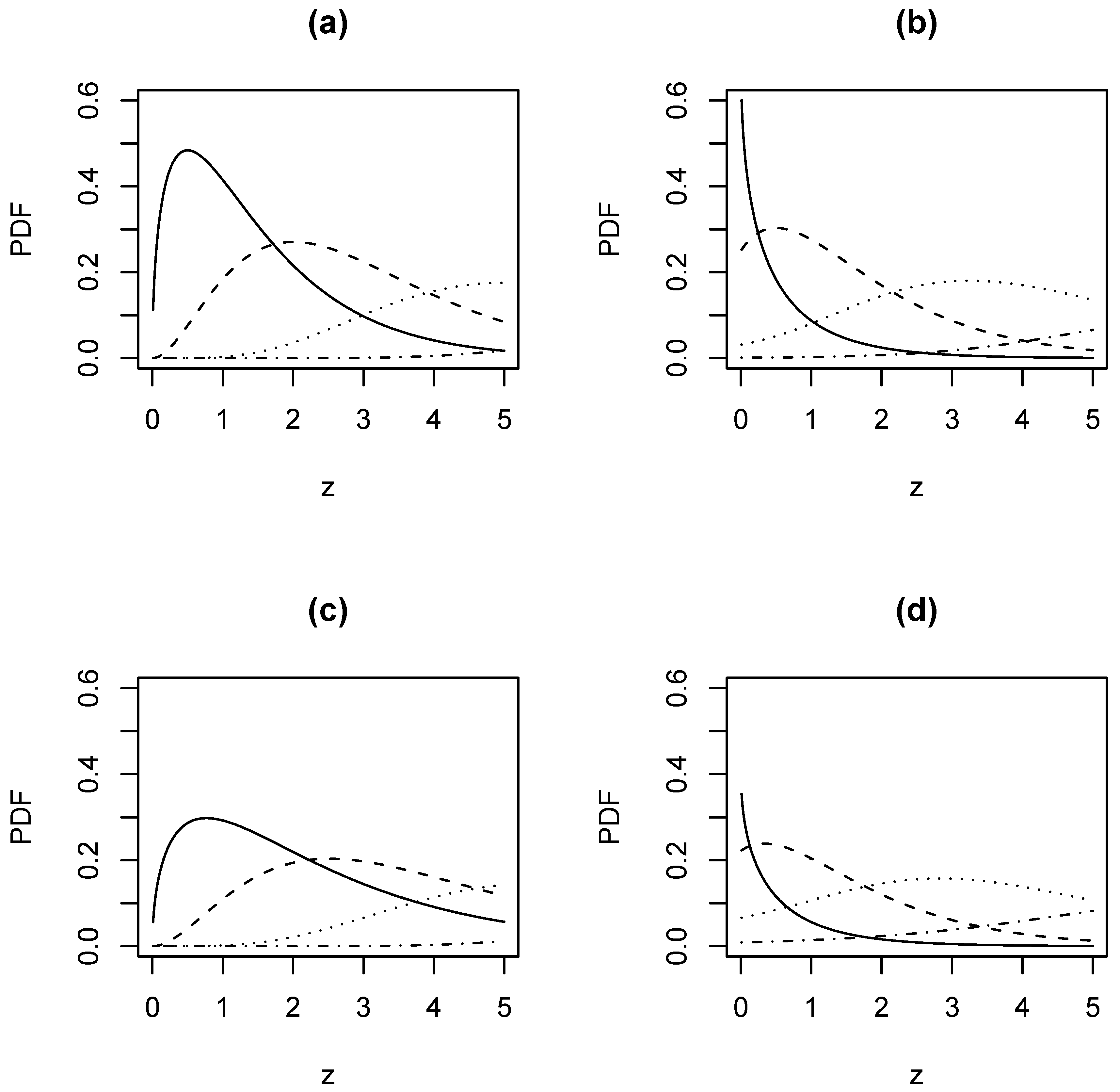
Figure 2.
Plots of the Shannon entropy for λ = 1, µ = 1, β = 1, α = 2, 3, . . . , 10 and a = 0.1, 0.2, . . . , 10 (left); for λ = 1, µ = 1, α = 2, β = −1, −2, . . . , −9 and a = 0.1, 0.2, . . . , 10 (right). The curves in the top plot from the bottom to the top correspond to increasing values of α. The curves in the bottom plot from the left to the right correspond to increasing values of β.
© 2005 by MDPI (http://www.mdpi.org). Reproduction for noncommercial purposes permitted.
Share and Cite
MDPI and ACS Style
Nadarajah, S.; Kotz, S. On the Linear Combination of Exponential and Gamma Random Variables. Entropy 2005, 7, 161-171. https://doi.org/10.3390/e7020161
AMA Style
Nadarajah S, Kotz S. On the Linear Combination of Exponential and Gamma Random Variables. Entropy. 2005; 7(2):161-171. https://doi.org/10.3390/e7020161
Chicago/Turabian StyleNadarajah, Saralees, and Samuel Kotz. 2005. "On the Linear Combination of Exponential and Gamma Random Variables" Entropy 7, no. 2: 161-171. https://doi.org/10.3390/e7020161