Quality Assessment of Gentiana rigescens from Different Geographical Origins Using FT-IR Spectroscopy Combined with HPLC


1
Institute of Medicinal Plants, Yunnan Academy of Agricultural Sciences, Kunming 650200, China
2
Yunnan Technical Center for Quality of Chinese Materia Medica, Kunming 650200, China
3
College of Traditional Chinese Medicine, Yunnan University of Traditional Chinese Medicine, Kunming 650500, China
*
Author to whom correspondence should be addressed.
Molecules 2017, 22(7), 1238; https://doi.org/10.3390/molecules22071238
Submission received: 9 June 2017
/
Accepted: 21 July 2017
/
Published: 24 July 2017
Abstract
:Gentiana rigescens is a precious herbal medicine in China because of its liver-protective and choleretic effects. A method for the qualitative identification and quantitative evaluation of G. rigescens from Yunnan Province, China, has been developed employing Fourier transform infrared (FT-IR) spectroscopy and high performance liquid chromatography (HPLC) with the aid of chemometrics such as partial least squares discriminant analysis (PLS-DA) and support vector machines (SVM) regression. Our results indicated that PLS-DA model could efficiently discriminate G. rigescens from different geographical origins. It was found that the samples which could not be determined accurately were in the margin or outside of the 95% confidence ellipses. Moreover, the result implied that geographical origins variation of root samples were more obvious than that of stems and leaves. The quantitative analysis was based on gentiopicroside content which was the main active constituent in G. rigescens. For the prediction of gentiopicroside, the performances of model based on the parameters selected through grid search algorithm (GS) with seven-fold cross validation were better than those based on genetic algorithm (GA) and particle swarm optimization algorithm (PSO). For the SVM-GS model, the result was satisfactory. FT-IR spectroscopy coupled with PLS-DA and SVM-GS can be an alternative strategy for qualitative identification and quantitative evaluation of G. rigescens.
1. Introduction
Herbal products, a complementary and alternative therapy, are increasingly gaining popularity in daily life and health care all over the world [1]. In the Western world, herbal medicine is mainly applied in promoting health and treatment of chronic diseases. It also plays a crucial role in multi-component therapeutics [2]. With the increasing usages of herbal medicine, the need for quality control has also increased. Currently, the regulations and pharmacovigilance about herbal medicines are still incomplete and need to be enhanced and improved [1,3]. The issues of quality control such as lack of safety and efficacy in herbal medicine are worthy of attention, because of the lack of reliable, fast and simple technical methods for the quality analysis of herbal medicines [4,5].
Gentiana rigescens (family Gentianaceae) is a precious and highly appreciated Chinese herbal medicine, which is widely distributed in the southwest of China, especially in Yunnan Province [6]. As a perennial herb, the root and rhizome are used as the primary medicinal part. This medicine mainly contains iridoids, lignans, triterpenes and others [7]. Among them, gentiopicroside, which belongs to the iridoid class of compounds, is the main active constituents of G. rigescens and it is recorded in Chinese Pharmacopoeia (version 2015) as a quality criterion [8]. This compound has long been used in the treatment of hepatic and cholalic diseases, as it has liver-protective and choleretic functions [9].
To our best knowledge, there are many external factors which can influence the quality of herbal medicines, such as geographical origin, harvest time, processing methods, etc. [10,11,12]. According to Yu et al. [13], traditional Chinese medicines and constitutional medicines from China, Japan and Korea differ due to geographical, social environment and other factors. The secondary metabolite composition of herbal medicines varies due to different geographical factors [14,15]. For example, Xia et al. [16] found that phenylalanine, tryptophan, chlorogenic acid syringin and lobetyolin levels in Codonopsis lanceolata samples were different depending on the geographical origin and harvesting time. Therefore, with its wide spectrum of therapeutic properties, it is crucial to provide guidance for the quality control of G. rigescens.
The conventional analytical methods for qualitative and quantitative analysis usually require operative skills, experience and are labor-intensive in addition to involving organic solvents for sample preparation. In this research, FT-IR spectroscopy, which is fast, clean and cost-effective, was developed to obtain chemical information about G. rigescens. It can provide qualitative information about the molecular structure of the components in G. rigescens with little or no sample pretreatment [17,18]. In addition, FT-IR spectroscopy, as a powerful analytical technique, has been widely used in the field of qualitative identification and quantitative evaluation in Chinese herbal medicines [19,20]. For these studies, FT-IR spectroscopy combined with multivariate analysis techniques has been applied to identify G. rigescens from different geographical origins and determine the iridoids in G. rigescens, and the results showed that FT-IR spectroscopy was suitable to provide qualitative and quantitative analyses of G. rigescens [21,22]. Similarly, Qi et al. [23], developed a HPLC and FTIR quantitative and qualitative analysis method to distinguish G. rigescens samples from different parts and cultivation years.
The objective of this study was to provide an efficient, easy-to-operate and non-hazardous alternative to evaluate the quality variation in different parts of G. rigescens from Dali, Lijiang, Diqing and Yuxi in Yunnan Province. Therefore, a method for the qualitative and quantitative analysis of G. rigescens has been developed employing FT-IR spectroscopy and chemometrics methods such as partial least squares discriminant analysis (PLS-DA) and support vector machines (SVM) regression. The results of gentiopicroside content determined by high performance liquid chromatography (HPLC) have been used as reference data to build our quantitative analysis model.
2. Result and Discussion
2.1. HPLC Analysis
All 179 samples were quantified by the HPLC method. Prior to sample determination, the methodology was validated by measuring the stability, repeatability and recovery based on the previous work in our laboratory [24]. The linear relationship of the peak areas and standards of gentiopicroside was y = 7975.52946x + 25.05267, and the correlation coefficient was 0.9999. Therefore, the HPLC method could be considered an accurate and dependable method for measuring gentiopicroside content in G. rigescens.
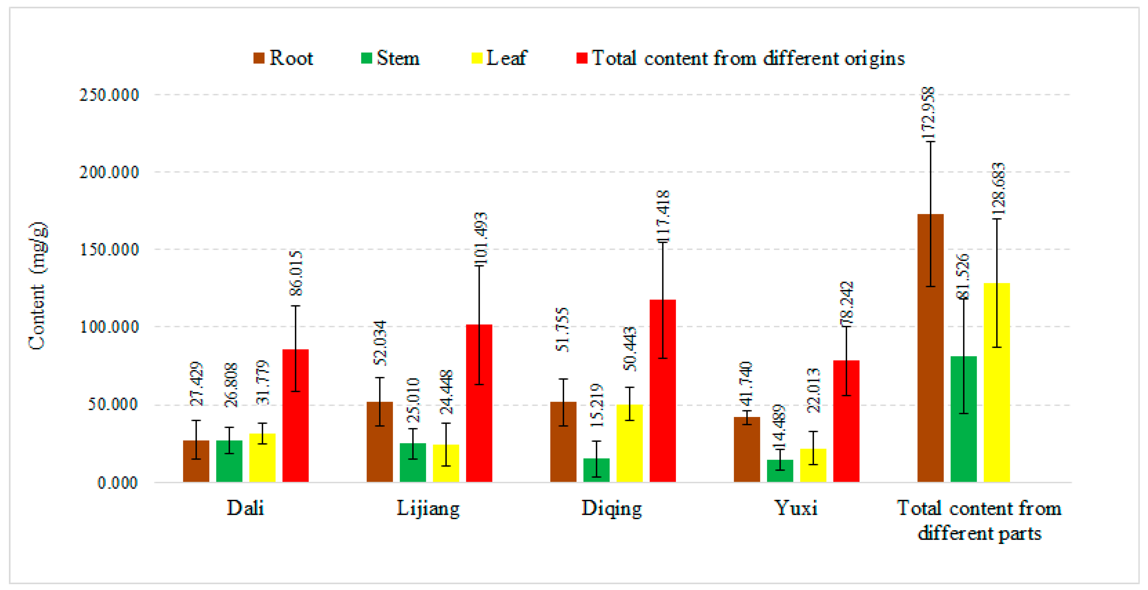
Figure 1 shows the average contents of gentiopicroside in different parts of G. rigescens from different geographical origins. For the date it can be concluded that samples from Diqing have the greatest gentiopicroside content, followed by those from Lijiang, Dali and Yuxi. Except for the samples from Dali which had the highest gentiopicroside content in leaf, the other three sources showed the highest abundance of gentiopicroside in the roots. It was thus found that not only in the same parts from different geographical origins but also the same part from different geographical origins, the content of gentiopicroside varies greatly. In addition, all samples conformed to the quality standards in the Chinese Pharmacopoeia except the stems from Yuxi (the content of gentiopicroside should be higher than 1.5%).
The above results show that G. rigescens samples show a great dependence on geographical origin, which might be influenced by the conditions of these geographical origins. For example, Yuxi is in the central part of Yunnan Province which is mainly a subtropical area, while the others are in the northwest of Yunnan Province, which belongs to the temperate climate zone area [25]. This indicates that the quality of the herb showed geographical and habitat dependences to some extent. Similar results have been reported for the quality of Paris from different geographic origins [26].
2.2. FT-IR Spectral Features
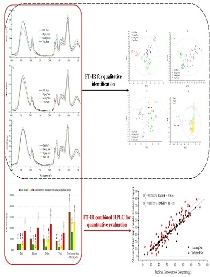
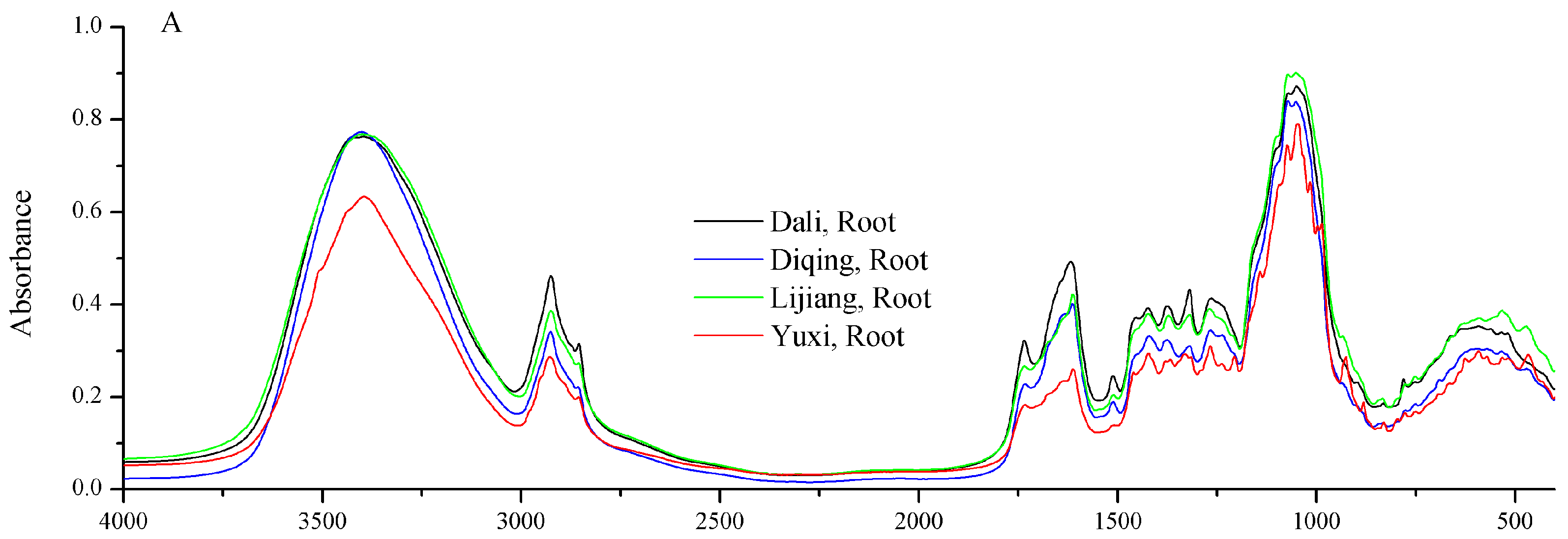
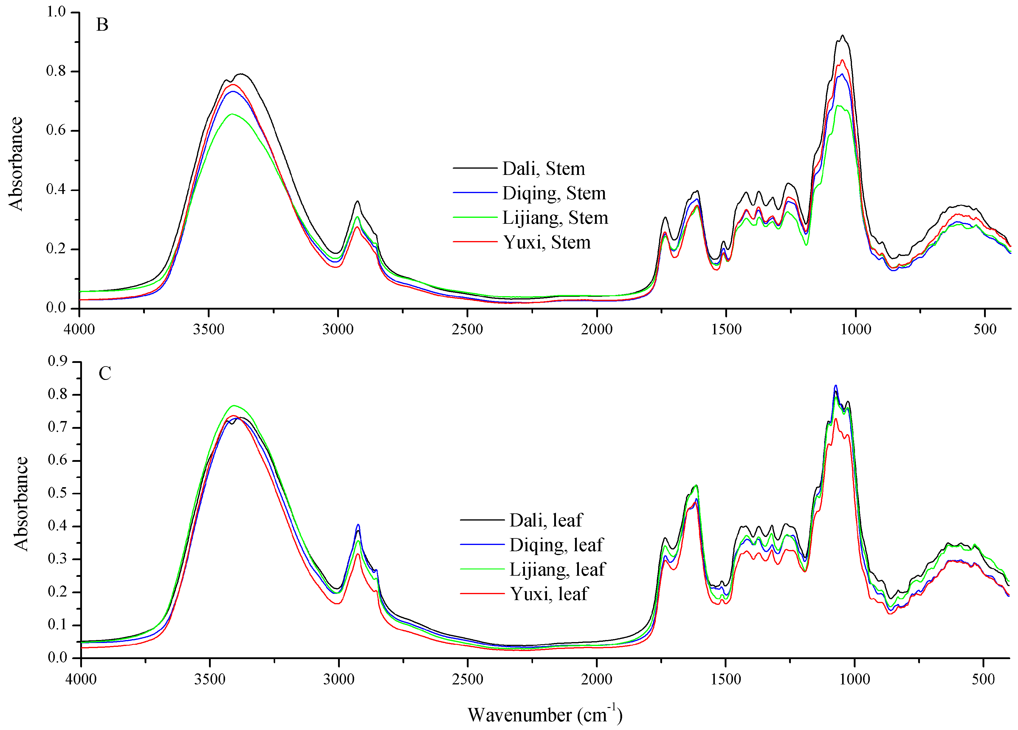
The average 4000–400 cm−1 FT-IR spectra of different parts of G. rigescens from different geographical origins are shown in Figure 2. On the whole, there is no distinct difference among the average FT-IR spectra, which overlap. However, the absorption intensities of the average FT-IR spectra vary a lot. Compared to other geographical origins, the absorption intensity is obviously lower in the root sample of Yuxi (Figure 2A). A broad absorption band is found at around 3399 cm−1, which is due to the O–H stretch. The bands at 2933 and 2856 cm−1 are CH3 asymmetric stretching and stretching vibration of esters, respectively. The peak around 1937 cm−1 is assigned to the C=O stretching vibration of acid amides [27]. In addition, the intense absorption peaks in 1070 and 1619 cm−1 are the main absorption bands of iridoids or glycosides, which correspond to C–O or C–O–C stretching and C–C asymmetric stretching vibrations [28,29]. According to studies of G. rigescens by Mi et al. [29] and Yang et al. [30], the active compounds gentiopicroside, swertiamarin, and chiratin and other iridoids in G. rigescens all contain C–O or C–O–C and C–C bonds.
2.3. Multivariate Analysis
In the PLS-DA and SVM regression models, the samples were divided into two categories: training set and validation set. Two-thirds of the samples were classified as training set and the others were assigned to the validation set by the Kennard-Stone algorithm [31].
2.3.1. PLS-DA Models
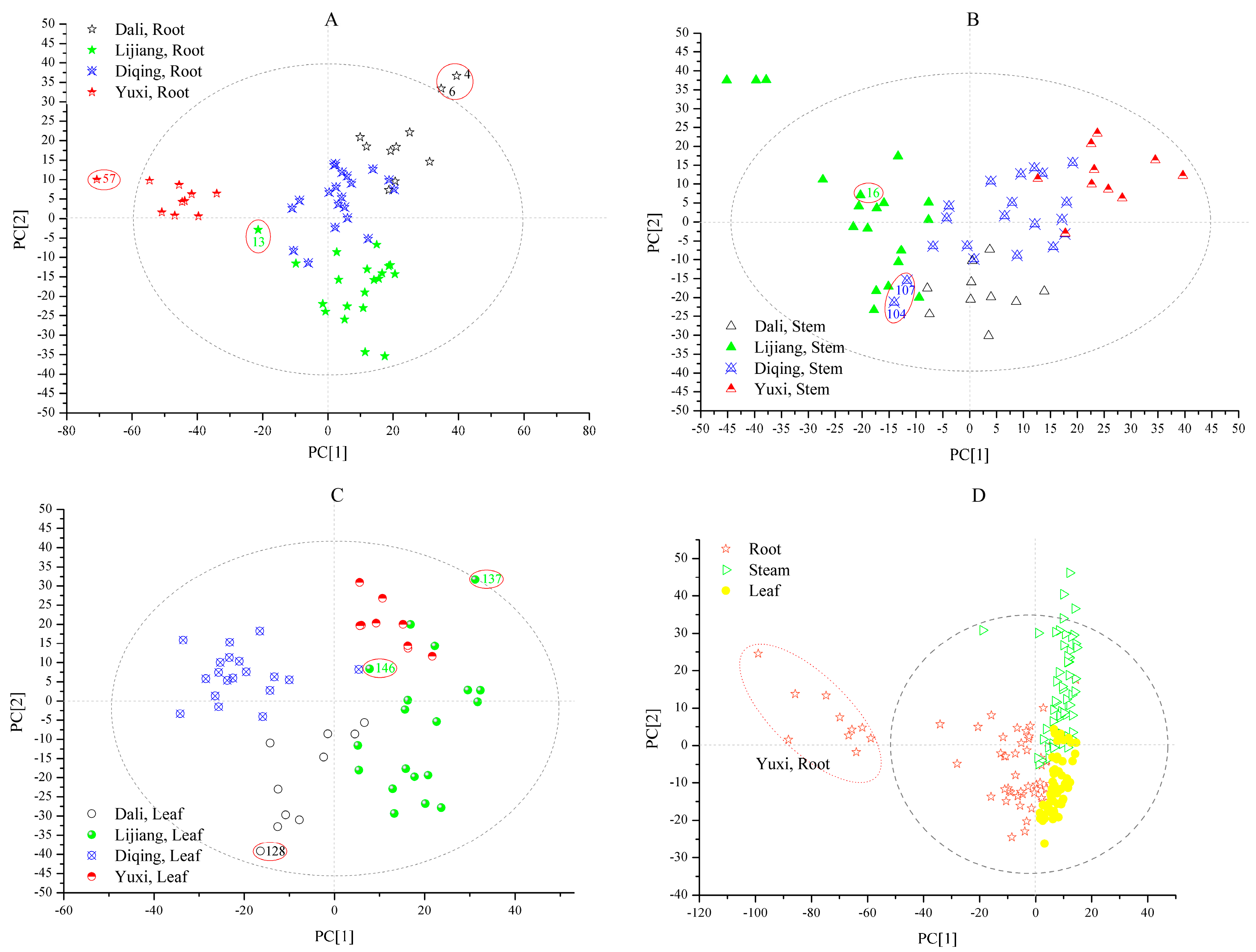
Four PLS-DA models were built: roots from different geographical origins (model 1), stems from different geographical origins (model 2), leafs from different geographical origins (model 3) and three different parts (root, stem and leaf) (model 4). In order to solve the problem of band overlap, baseline drift and noise, spectral preprocessing was applied [32,33,34]. For the PLS-DA models 1, 2, 3 and 4, the optimized spectral preprocessing were second derivation (2Der), multiplicative scatter correction (MSC) + 2Der, standard normal variate (SNV) + 2Der and MSC + 2Der, respectively. After optimized spectral preprocessing of the FT-IR spectra, the PLS-DA models were established by the first two principal components (PC1 and PC2) for qualitative analysis of all G. rigescens samples (Figure 3).
Figure 3A displays the score plot of G. rigescens roots from Dali, Lijiang, Diqing and Yuxi. In the score plot, samples from different geographical origins can be clustered in a range and distinguished from others. Samples from Yuxi are far away from the other three geographical origins, while the distance of the other three geographical origins are closer. It can be seen that PC1 separates the samples of Yuxi from others, the former is in the central of Yunnan Province and the latter is in the northwest of Yunnan Province, which matches the regularities of gentiopicroside content distribution analyzed by HPLC. PC2 separates the samples of Diqing and Dali from samples of Lijiang.
The prediction results of the model parameters determination coefficient (R2), root-mean-square error of estimation (RMSEE) and root-mean-square error of cross validation (RMSECV) are listed in Table 1. The first six principal components (96.0%) are employed for model 1. The R2 is greater than 0.94 and the RMSEE and RMSECV are low, which are less than 0.25. Thereinto, model 1 of samples from Yuxi have the best performance with the highest R2 and lowest RMSEE and RMSECV. As seen in Table 2, according to the Galtier criterion, all the samples are identified correctly except the four samples numbered 4, 6, 13 and 57. Sample 13 from Lijiang was misidentified as coming from Diqing, and the three other samples (4, 6 and 57) can’t be judged accurately. More interestingly, the uncertain samples are all outside of the 95% confidence ellipses in the scatter plot (Figure 3A). The prediction accuracy of model 1 is 80%.
The score plot of G. rigescens stems from Dali, Lijiang, Diqing and Yuxi is described in Figure 3B. The G. rigescens stems from different geographical origins can be separated except for a few that were mixed. The stems from Lijiang are distributed widely, while the samples from the other three origins are centrally distributed. It is shown that PC1 separates the samples of Lijiang and Yuxi from those of Dali and Diqing while PC2 separates the samples of Dali from those from Diqing.
Table 1 shows the parameters of R2, RMSEE and RMSECV in model 2. The first four principal components are employed for model 2, and the cumulative contribution reached 88.5%. The model of samples from Yuxi have the best precision, with high R2 (0.9472) and low RMSEE (0.0877) and RMCECV (0.1689).
According to the Galtier criterion, two samples from Diqing (104 and 107) are identified as Lijiang samples erroneously and sample 76 can’t be judged accurately (Table 3). As seen in Figure 3B, samples 104 and 107 are close to the samples from Lijiang which is the same as the results from Table 3. The prediction accuracy of model 2 is 85%.
Figure 3C displays the score plots of G. rigescens leaves from Dali, Lijiang, Diqing and Yuxi. The cumulative contribution reached 90.2%, when the first four principal components are employed. In Figure 3C, the samples from Dali, Diqing and Yuxi can be clustered into three groups, while Lijiang samples are distributed dispersedly. The samples from Diqing and Dali can be separated from the Yuxi and Lijiang ones by PC1. In addition, the samples from Yuxi and Lijiang can be distinguished by PC2.
The R2, RMSEE and RMSECV of model 3 are shown in Table 1. The performances of the different geographical origin discrimination are good, with high R2 (>0.88) and low RMSEE (<0.17) and RMSECV (<0.20). Thereinto, the best performance is for the samples from Yuxi. In Table 4, the samples 128 and 137 can’t be confirmed. Moreover, a sample from Lijiang (146) is judged as a Dali sample by mistake. More interestingly, the uncertain samples are in the margin of the 95% confidence ellipses (Figure 3C) like the result of model 1. The prediction accuracy of model 3 is 85%.
The score plot (Figure 3D) shows that all G. rigescens samples can be separated based on three parts (root, stem and leaf). The first four principal components which represent 87.0% of the explained variance are applied to model 4. It is clear that the roots, stems and leaves can be separated completely. Thia indicates that the metabolic profiles of different parts in G. rigescens are unlike. The stems and leaves samples cluster in two concentrated regions and the distance between them is close, however, the root samples distribute dispersedly whereby the root samples from Yuxi cluster outside the 95% confidence ellipses and the distance between the roots samples from Yuxi and the other root samples are large (Figure 3D). This indicates that the geographical origins variation of root samples are more obvious than those of stems and leaves. Moreover, it is shown that PC1 separates the root samples from stem and leaf samples and PC2 separates the stem samples from leaf samples.
As shown in Table 1, the best performance of model 4 is leaf samples, followed by stem and root. The prediction accuracy of model 3 is 86.7%, which six samples (29, 51, 61, 62, 106 and 111) are uncertain whether class belongs to, and three stem samples (63, 78 and 83) are regarded as root samples (Table 5). The result shows that the metabolic profiles of leaf samples may be similar to root samples.
2.3.2. SVM Regression Model
After optimized spectral preprocessing by orthogonal signal correction (OSC) and 2Der, all data was normalized in the region between 1 and 2. Then, the parameters c and g in the SVM regression model were selected by a grid search algorithm (GS) with seven-fold cross validation, genetic algorithm (GA) and particle swarm optimization algorithm (PSO). The GS with cross-validation can prevent the problem of overfitting and can be easily parallelized on account of parameters (c and g) [35]. The algorithm of GA is based on the principle of survival of the fittest. In GA algorithm, the most obvious superiority is that it can find the optimal or near the optimal solutions in the relatively low computation [36]. The basic concept of PSO algorithm is derived from the study of bird predation behavior. It is a new stochastic optimization algorithm based on the intelligent [37]. Finally, the best parameters were used to train the training set.
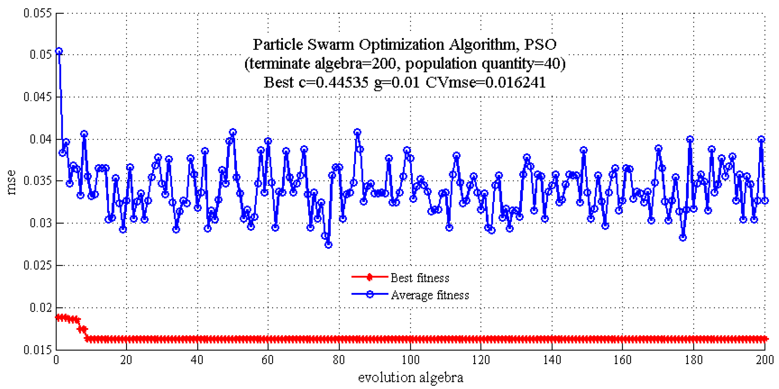
In this study, the GS algorithm was applied to screen the parameters c and g in the region of 1 to 220 and 2−20 to 1, respectively. As can be seen in Figure 4, the results of c, g and cross-validation mean square error (CVmse) which are calculated by the GS algorithm are 0.5, 0.0039 and 0.0149, respectively. In addition, the terminate algebra was set as 200 and population quantity was set as 40 in the GA algorithm. It is shown that the optimum parameters c, g and CVmse are 0.4572, 0.01 and 0.0163, respectively (Figure 5). Finally, the PSO algorithm was also applied to select the parameters and the detail parameter (terminate algebra and population quantity) of PSO was the same as the GA algorithm (Figure 6). The results of the PSO algorithm are as follows: c = 0.4453, g = 0.01 and CVmse = 0.01624. The aforementioned algorithms were all applied for building the SVM regression models.
Table 6 shows the performances achieved by the GS, GA and PSO SVM regression models for predicting the content of gentiopicroside. From Table 6, it is observed that the highest Rt2 (96.39%) and RMSEE (3.1056) for training set and the highest Rv2 (83.57%) and the lowest RMSEP (11.1421) for validation set is obtained by the GS algorithm. Therefore, the GS method gives the best performance for the prediction of gentiopicroside content in G. rigescens.
Figure 7 shows the result of validation set for prediction vs. measured gentiopicroside content which was achieved by the GS algorithm in the SVM regression model. The samples from the training and validation sets are all symmetrically distributed on the both sides of the regression line. Satisfactory predictions with Rt2, Rt2, RMSEE and RMSEP are achieved and good agreement with the SVM regression model built for predicting gentiopicroside content in G. rigescens is observed.
3. Materials and Methods
3.1. Plant Materials and Reagents
Wild fresh G. rigescens samples were collected from Dali, Lijiang, Diqing and Yuxi in Yunnan Province, China (Table 7). Specimens were identified by Prof. Jinyu Zhang (Institute of Medicinal Plants, Yunnan Academy of Agricultural Sciences).
Potassium bromide (KBr) was purchased from Tianjin Fengchuan Fine Chemical Research Institute (Tianjin, China). A gentiopicroside standard was supplied by the National Institute for the Control of Food and Drug control (Beijing, China). Analytical grade methanol (80%, v/v) used as extraction solvent was obtained from Xilong Chemical Company (Guangdong, China). Chromatography grade acetonitrile and formic acid were purchased from Sigma-Aldrich (Flanders, NJ, USA).
3.2. Sample Preparation
The G. rigescens samples were divided into three parts (root, stem and leaf) after cleaning and dried for 24 h at 60 °C. Then, all samples were powdered in a high-speed blender and passed through an 80 mesh stainless steel sieve, separately. Then, the sieved powders were kept in Ziploc bags and stored at room temperature prior to analysis.
A sample (25 mg) of each powder was weighed accurately using an electronic balance (XS125A, Precisa, Basel, Switzerland) and soaked with 1.5 mL of 80% methanol for 30 min under ultrasonication at room temperature. Before analysis by HPLC, the extracts were filtered through a 0.22 μm membrane filter (Millipore, Bedford, MA, USA). All the extracts of G. rigescens samples were subjected to analysis.
3.3. HPLC Conditions
Gentiopicroside was determined using an Agilent 1260 Infinity system (Agilent Technologies, Palo Alto, CA, USA) equipped with a G1311 diode array detector, a quaternary pump and an on-line degasser. An Agilent Zorbax AB-C18 column (5 µm, 4.6 × 250 mm) was utilized for the chromatographic separations. The mobile phase consisted of 0.1% aqueous formic acid in water (A) and acetonitrile (B). The gradient elution procedure was as follows: the initial mobile phase composition was set to 5% B for 5 min, then increased stepwise linearly first to 10% B from 5 to 10 min, then to 26% B from 10 to 26 min, and finally decreased to 30% for 30 min. The column temperature was maintained at 30 °C. The flow rate was set at 0.3 mL/min and the injection volume was 10 µL. During the experiment, the detective wavelength was set at 241 nm. Every samples were detected three times, and the averaged spectra were employed for further analysis.
3.4. FT-IR Spectra Acquisition
FT-IR spectra acquisition was performed by using a Fourier transform infrared spectrometer (Perkin Elmer, Norwalk, CT, USA) equipped with a deuterated triglycine sulfate detector. Powdered samples (1.2 mg) and 100 mg of KBr were precisely weighed and mixed evenly. Then, the mixed powder was pressed into a tablet by using a table press (YP-2, Shanghai Shanyue Instrument Inc., Shanghai, China) for detection. Each FT-IR spectrum was collected in the region of 4000–400 cm−1 with a resolution of 4 cm−1 and a total of 16 co-added scans. Pure KBr spectra were recorded as background spectra for deducting the CO2 and H2O peaks in real-time. Each spectrum was scanned in triplicate under constant temperature (25 °C) and humidity conditions, and the averaged spectra were employed for further analysis.
3.5. Multivariate Data Analysis
Before analysis, two-thirds of the samples were classified as the training set and the others were assigned to the validation set using the Kennard-Stone algorithm. Qualitative and quantitative models were developing with PLS-DA and SVM regression, respectively. PLS-DA, a supervised analysis method, was successfully applied to the classification of the FT-IR spectra [38]. The basic principle of PLS-DA was to reduce the independent variables X for obtaining a maximum covariance between X and Y variables [39,40]. SVM, a state-of-the-art method of classification and regression technique, was proposed on the basis of statistical learning theory by Vapnik [41]. The fundamental objective of SVM was to construct a separating plane that all the data points have the shortest distance to [42]. SVM is famous for its advantages which avoid over-fitting problems and improve the generalization and accurate prediction ability by introducing a structure risk function. Rather than empirical risk that minimizes the misclassification errors in the training set, structural risk minimizes the misclassification error on a settled but unware probability distribution in which previously invisible data points are drawn at random [43,44]. Moreover, SVM can effectively overcome the “curse of dimensionality” by introducing a kernel function. SVM thus successfully solves non-linear prediction problems [45].
In this paper, a library for the SVM toolkit LIBSVM 3.21 was applied in data processing which was developed by Chang and optimized by Lin [46]. The performance of SVM depends mainly on the type of kernel function and its parameters [47]. There are four kinds of kernel function types in this toolkit, including: linear, radial basis function (RBF), polynomial and sigmoid. Usually, RBF is selected to build the regression models for prediction [42,48,49]. The error penalty parameter c and RBF kernel parameter g are the major parameters in the SVM model with RBF [50]. The RBF kernel parameter g, as kernel width, had an impact on the prediction of the SVM model, while c controls the complexity of the SVM model.
3.6. Evaluation of Model Performance
The determination coefficient (R2), root-mean-square error of estimation (RMSEE), root-mean-square error of cross validation (RMSECV) and root-mean-square error of prediction (RMSEP) were considered to evaluate the performance of qualitative and quantitative model.
R2 (Equation (1)) is the correlation between the measured values and predicted values. Generally, a higher R2 (<1) value means a better performance of both kinds of models [51]:
where, yi is the measured value while ŷi is the predicted value. is the mean value, and N is the number of samples.
RMSEE, RMSECV and RMSEP were applied to evaluate the precision of model performance (Equations (2)–(4)). The lower RMSEE, RMSECV and RMSEP are, the fitter the models obtained [52,53,54]. Moreover, the robustness of models depends on the difference between the determination coefficient for the training set () and the determination coefficient for the validation set (). The smaller the difference between them, the more satisfactory the model [55]:
where, Nt is the number of the training set and Nv is the number of validation set. In addition, in the qualitative model, the classification accuracy of the validation set depends on the predicted value (Ypre), and deviation values (Ydev) which are based on the following standards: (1) when Ypre > 0.5 and Ydev < 0.5, the sample of validation set belongs to the class; (2) when Ypre < 0.5 and Ydev < 0.5, the sample of validation set does not belong to the class; (3) when Ydev > 0.5, it means that the sample can’t judge accurately whether it belongs to the class or not [56,57].
3.7. Software
The FT-IR spectra were processed using Omnic (Version 8.2, Thermo Fisher Scientific, Madison, WI, USA). The chromatographic fingerprints were conducted using the Similarity Evaluation System for Chromatographic Fingerprints of traditional Chinese Medicines (Version 2004a, Chinese Pharmacopoeia Commission, Beijing, China). The PLS-DA models were created by Simca (Version 13.0, Umetrics, Umea, Sweden), while the MSV regression model was created by MATLAB (Version R2014a, MathWorks, Natick, MA, USA) with the LIBSVM-Faruto toolkit (Version Ultimate 3.1M) [58]. All the figures were drawn by Origin (Version 8.0, Originlab, North Hampton, MA, USA) and MATLAB.
4. Conclusions
In this study, a rapid FT-IR spectroscopic method combined with a chemometrics procedure was developed for the qualitative and quantitative analysis of G. rigescens. The discrimination of different parts of G. rigescens plants from different geographical origins by using FT-IR spectroscopy in combination with PLS-DA was presented. The feasibility of rapid quantitative analysis of gentiopicroside content in G. rigescens by application of FT-IR spectroscopy in combination with SVM regression was investigated. The results showed that for gentiopicroside determination, the parameter selection method of GS of a SVM regression model provided a good prediction. Overall, FT-IR spectroscopy combined with chemometrics could be a promising method for quality assessment of G. rigescens.
Acknowledgments
This work was supported by the National Natural Science Foundation of China (Grant No. 81660638) and Key Project of Yunnan Provincial Natural Science Foundation (Targeted & non-targeted metabonomics study for accumulation of active ingredients and distribution diversity in Gentiana rigescens).
Author Contributions
Zhe Wu and Ji Zhang conceived and designed the experiments; Zhe Wu performed the experiments; Zhe Wu and Yanli Zhao analyzed the data; Yuanzhong Wang contributed reagents/materials/analysis tools; Zhe Wu wrote the paper.
Conflicts of Interest
The authors declare no conflict of interest.
References
- Licata, A.; Macaluso, F.S.; Craxì, A. Herbal hepatotoxicity: A hidden epidemic. Intern. Emerg. Med. 2013, 8, 13–22. [Google Scholar] [CrossRef] [PubMed]
- Choi, Y.H.; Chin, Y.W.; Kim, Y.G. Herb-drug interactions: Focus on metabolic enzymes and transporters. Arch. Pharm. Res. 2011, 34, 1843–1863. [Google Scholar] [CrossRef] [PubMed]
- Gad, H.A.; El-Ahmady, S.H.; Abou-Shoer, M.I.; Abou-Shoerb, M.I.; Al-Azizi, M.M. Application of chemometrics in authentication of herbal medicines: A review. Phytochem. Anal. 2013, 24, 1–24. [Google Scholar] [CrossRef] [PubMed]
- Anderson, M.L.; Burney, D.P. Validation of sample preparation procedures for botanical analysis. J. AOAC Int. 1998, 81, 1005–1010. [Google Scholar]
- Huie, C.W. A review of modern sample-preparation techniques for the extraction and analysis of medicinal plants. Anal. Bioanal. Chem. 2002, 373, 23–30. [Google Scholar] [CrossRef] [PubMed]
- State Pharmacopoeia Commission. Chinese Pharmacopoeia; China Medical Science and Technology Press: Beijing, China, 2015; Volume I, pp. 260–261. [Google Scholar]
- Pan, Y.; Zhang, J.; Shen, T.; Zuo, Z.T.; Jin, H.; Wang, Y.Z.; Li, W.Y. Optimization of ultrasonic extraction by response surface methodology combined with ultrafast liquid chromatography–ultraviolet method for determination of four iridoids in Gentiana rigescens. J. Food Drug Anal. 2014, 23, 529–537. [Google Scholar] [CrossRef]
- Xu, M.; Wang, D.; Zhang, Y.J.; Yang, C.R. Dammarane triterpenoids from the roots of Gentiana rigescens. J. Nat. Prod. 2007, 70, 880–883. [Google Scholar] [CrossRef] [PubMed]
- Zhang, X.D.; Allan, A.C.; Li, C.X.; Wang, Y.Z.; Yao, Q.Y. De Novo assembly and characterization of the transcriptome of the Chinese medicinal herb, Gentiana rigescens. Int. J. Mol. Sci. 2015, 16, 11550–11573. [Google Scholar] [CrossRef] [PubMed]
- Melito, S.; Petretto, G.L.; Podani, J.; Foddai, M.; Maldini, M.; Chessa, M.; Pintore, G. Altitude and climate influence Helichrysum italicum subsp. microphyllum essential oils composition. Ind. Crops Prod. 2016, 80, 242–250. [Google Scholar] [CrossRef]
- Wu, Z.; Zhang, J.; Xu, F.R.; Wang, Y.Z.; Zhang, J.Y. Rapid and simple determination of polyphyllin I, II, VI, and VII in different harvest times of cultivated Paris polyphylla Smith var. yunnanensis (Franch.) Hand.-Mazz by UPLC-MS/MS and FT-IR. J. Nat. Med. 2017, 71, 139–147. [Google Scholar] [CrossRef] [PubMed]
- Shu, X.; Jiang, X.W.; Cheng, B.C.Y.; Ma, S.C.; Chen, G.Y.; Yu, Z.L. Ultra-performance liquid chromatography-quadrupole/time-of-flight mass spectrometry analysis of the impact of processing on toxic components of Kansui Radix. BMC Complement. Altern. Med. 2016, 16, 73. [Google Scholar] [CrossRef] [PubMed]
- Yu, W.J.; Ma, M.Y.; Chen, X.M.; Li, L.R.; Zheng, Y.F. Traditional Chinese Medicine and Constitutional Medicine in China, Japan and Korea: A Comparative Study. Am. J. Chin. Med. 2017, 45, 1–12. [Google Scholar] [CrossRef] [PubMed]
- Jing, P.; Zhao, S.J.; Lu, M.M.; Cai, Z.; Pang, J.; Song, L.H. Multiple-fingerprint analysis for investigating quality control of Flammulina velutipes fruiting body polysaccharides. J. Agric. Food Chem. 2014, 62, 12128–12133. [Google Scholar] [CrossRef] [PubMed]
- Choong, Y.K.; Xu, C.H.; Lan, J.; Chen, X.D.; Jamal, J.A. Identification of geographical origin of Lignosus samples using Fourier transform infrared and two-dimensional infrared correlation spectroscopy. J. Mol. Struct. 2014, 1069, 188–195. [Google Scholar] [CrossRef]
- Xia, Y.Y.; Liu, F.L.; Feng, F.; Liu, W.Y. Characterization, quantitation and similarity evaluation of Codonopsis lanceolata from different regions in China by HPLC-Q-TQF-MS and chemometrics. J. Food Compos. Anal. 2017, 62, 134–142. [Google Scholar] [CrossRef]
- Kaniu, M.I.; Angeyo, K.H.; Mwala, A.K.; Mangala, M.J. Direct rapid analysis of trace bioavailable soil macronutrients by chemometrics-assisted energy dispersive X-ray fluorescence and scattering spectrometry. Anal. Chim. Acta 2012, 729, 21–25. [Google Scholar] [CrossRef] [PubMed]
- Shao, Q.S.; Zhang, A.; Ye, W.W.; Guo, H.P.; Hu, R.H. Fast determination of two atractylenolides in Rhizoma Atractylodis Macrocephalae by Fourier transform near-infrared spectroscopy with partial least squares. Spectrochim. Acta A Mol. Biomol. Spectrosc. 2014, 120, 499–504. [Google Scholar] [CrossRef] [PubMed]
- Chavez, P.F.; Sacre, P.Y.; De Bleye, C.; Netchacovitch, L.; Mantanus, J.; Motteb, H.; Schubert, M.; Hubert, P.; Ziemons, E. Active content determination of pharmaceutical tablets using near infrared spectroscopy as Process Analytical Technology tool. Talanta 2015, 144, 1352–1359. [Google Scholar] [CrossRef] [PubMed]
- Feng, Y.C.; Lei, D.Q.; Hu, C.Q. Rapid identification of illegal synthetic adulterants in herbal anti-diabetic medicines using near infrared spectroscopy. Spectrochim Acta A Mol. Biomol. Spectrosc. 2014, 125, 363–374. [Google Scholar] [CrossRef] [PubMed]
- Zhao, Y.L.; Zhang, J.; Jin, H.; Zhang, J.Y.; Shen, T.; Wang, Y.Z. Discrimination of Gentiana rigescens from different origins by Fourier transform infrared spectroscopy combined with chemometric methods. J. AOAC Int. 2015, 98, 22–26. [Google Scholar] [CrossRef] [PubMed]
- Qi, L.M.; Zhang, J.; Zuo, Z.T.; Zhao, Y.L.; Wang, Y.Z.; Jin, H. Determination of Iridoids in Gentiana rigescens by Infrared Spectroscopy and Multivariate Analysis. Anal. Lett. 2017, 50, 389–401. [Google Scholar] [CrossRef]
- Qi, L.M.; Zhang, J.; Zhao, Y.L.; Zou, Z.T.; Jin, H.; Wang, Y.Z. Quantitative and Qualitative Characterization of Gentiana rigescens Franch (Gentianaceae) on Different Parts and Cultivations Years by HPLC and FTIR Spectroscopy. J. Anal. Methods Chem. 2017, 2017, 3194146. [Google Scholar] [CrossRef] [PubMed]
- Shen, T.; Zhang, J.; Zhao, Y.L.; Zuo, Z.T.; Wang, Y.Z. Chemometric Analysis of the Stem and Leaf of Gentiana rigescens in Agroforestry Systems. Plant Sci. J. 2015, 33, 472–481. [Google Scholar]
- Cheng, J.G.; Wang, X.F.; Fan, L.Z.; Yang, X.P.; Yang, P.W. Variations of Yunnan climatic zones in recent 50 years. Prog. Geogr. 2009, 28, 18–24. [Google Scholar]
- Zhao, Y.L.; Zhang, J.; Yuan, T.J.; Shen, T.; Li, W.; Yang, S.H.; Hou, Y.; Wang, Y.Z.; Jin, H. Discrimination of wild Paris based on near infrared spectroscopy and high performance liquid chromatography combined with multivariate analysis. PLoS ONE 2014, 9, e89100. [Google Scholar] [CrossRef] [PubMed]
- Cheng, C.G.; Liu, J.; Cao, W.Q.; Zheng, R.W.; Wang, H.; Zhang, C.J. Classification of two species of Bidens based on discrete stationary wavelet transform extraction of FTIR spectra combined with probability neural network. Vib. Spectrosc. 2010, 54, 50–55. [Google Scholar] [CrossRef]
- Xu, M.; Wang, D.; Zhang, Y.J.; Yang, C.R. A new secoiridoidal glucoside from Gentiana rigescens (Gentianaceae). Acta Bot. Yunnanica 2006, 28, 669–672. [Google Scholar]
- Mi, L.J.; Zhang, J.; Zhao, Y.L.; Wang, Y.Z.; Li, F.S. Application of infrared spectroscopy for choosing drying methods of Gentiana rigescens. Lishizhen Med. Mater. Med. Res. 2015, 26, 2656–2659. [Google Scholar] [CrossRef]
- Yang, H.X.; Ma, F.; Du, Y.Z.; Sun, S.Q.; Wei, L.X. Study on the Tiabetan medicine Swertia mussotii Franch and its extracts by Fourier transform infrared spectroscopy. Spectrosc. Spectr. Anal. 2014, 34, 2973–2977. [Google Scholar]
- Kennard, R.W.; Stone, L.A. Computer aided design of experiments. Technometrics 1969, 11, 137–148. [Google Scholar] [CrossRef]
- Rinnan, Å.; van den Berg, F.; Engelsen, S.B. Review of the most common pre-processing techniques for near-infrared spectra. TRAC Trends Anal. Chem. 2009, 28, 1201–1222. [Google Scholar] [CrossRef]
- Maleki, M.R.; Mouazen, A.M.; Ramon, H.; De Baerdemaeker, J. Multiplicative scatter correction during on-line measurement with near infrared spectroscopy. Biosyst. Eng. 2007, 96, 427–433. [Google Scholar] [CrossRef]
- Guo, Q.; Wu, W.; Massart, D.L. The robust normal variate transform for pattern recognition with near-infrared data. Anal. Chim. Acta 1999, 382, 87–103. [Google Scholar] [CrossRef]
- Hsu, C.W.; Chang, C.C.; Lin, C.J. A Practical Guide to Support Vector Classification. 2003. Available online: http://www.csie.ntu.edu.tw/~cjlin/papers/guide/guide.pdf (accessed on 10 May 2017).
- Kalteh, A.M. Wavelet genetic algorithm-support vector regression (Wavelet GA-SVR) for monthly flow forecasting. Water Resour. Manag. 2015, 29, 1283–1293. [Google Scholar] [CrossRef]
- Cheng, Z.Y.; Kong, H.H.; Zhang, J.; Bai, W.L.; Gan, F. Application of Particle Swarm Optimization-Least Square Support Vector Machine Regression to Modeling of Near Infrared Spectra. J. Instrum. Anal. 2010, 12, 1215–1219. [Google Scholar] [CrossRef]
- Grasel, F.S.; Ferrão, M.F. A rapid and non-invasive method for the classification of natural tannin extracts by near-infrared spectroscopy and PLS-DA. Anal. Methods 2016, 8, 644–649. [Google Scholar] [CrossRef]
- Górski, Ł.; Sordoń, W.; Ciepiela, F.; Kubiak, W.W.; Jakubowska, M. Voltammetric classification of ciders with PLS-DA. Talanta 2016, 146, 231–236. [Google Scholar] [CrossRef] [PubMed]
- Dominguez-Vidal, A.; Pantoja-de la Rosa, J.; Cuadros-Rodríguez, L.; Ayora-Cañada, M.J. Authentication of canned fish packing oils by means of Fourier transform infrared spectroscopy. Food Chem. 2016, 190, 122–127. [Google Scholar] [CrossRef] [PubMed]
- Cortes, C.; Vapnik, V. Support-vector networks. Mach. Learn. 1995, 20, 273–297. [Google Scholar] [CrossRef]
- Yang, Y.; Liu, X.S.; Li, W.L.; Jin, Y.; Wu, Y.J.; Zheng, J.Y.; Zhang, W.T.; Chen, Y. Rapid measurement of epimedin A, epimedin B, epimedin C, icariin, and moisture in Herba Epimedii using near infrared spectroscopy. Spectrochim. Acta A Mol. Biomol. Spectrosc. 2017, 171, 351–360. [Google Scholar] [CrossRef] [PubMed]
- Chen, Q.S.; Zhao, J.W.; Fang, C.H.; Wang, D.M. Feasibility study on identification of green, black and Oolong teas using near-infrared reflectance spectroscopy based on support vector machine (SVM). Spectrochim. Acta A Mol. Biomol. Spectrosc. 2007, 66, 568–574. [Google Scholar] [CrossRef] [PubMed]
- Gunn, S.R. Support Vector Machines for Classification and Regression. ISIS Tech. Rep. 1998, 14, 85–86. [Google Scholar]
- Zhang, Y.; Cong, Q.; Xie, Y.F.; Yang, J.X.; Zhao, B. Quantitative analysis of routine chemical constituents in tobacco by near-infrared spectroscopy and support vector machine. Spectrochim. Acta A Mol. Biomol. Spectrosc. 2008, 71, 1408–1413. [Google Scholar] [CrossRef] [PubMed]
- Chang, C.C.; Lin, C.J. LIBSVM: A library for support vector machines. ACM Trans. Intell. Syst. Technol. 2011, 2, 27. [Google Scholar] [CrossRef]
- Subasi, A. Classification of EMG signals using PSO optimized SVM for diagnosis of neuromuscular disorders. Comput. Biol. Med. 2013, 43, 576–586. [Google Scholar] [CrossRef] [PubMed]
- Benkedjouh, T.; Medjaher, K.; Zerhouni, N.; Rechak, S. Health assessment and life prediction of cutting tools based on support vector regression. J. Intell. Manuf. 2015, 26, 213–223. [Google Scholar] [CrossRef] [Green Version]
- Ulenberg, S.; Belka, M.; Król, M.; Herold, F.; Hewelt-Belka, W.; Kot-Wasik, A.; Bączek, T. Prediction of overall in vitro microsomal stability of drug candidates based on molecular modeling and support vector machines. Case study of novel arylpiperazines derivatives. PLoS ONE 2015, 10, e0122772. [Google Scholar] [CrossRef] [PubMed]
- Liu, M.; Wang, M.; Wang, J.; Dou, L. Comparison of random forest, support vector machine and back propagation neural network for electronic tongue data classification: Application to the recognition of orange beverage and Chinese vinegar. Sens. Actuators B Chem. 2013, 177, 970–980. [Google Scholar] [CrossRef]
- Zhong, J.F.; Qin, X.L. Rapid quantitative analysis of corn starch adulteration in Konjac Glucomannan by chemometrics-assisted FT-NIR spectroscopy. Food Anal. Methods 2016, 9, 61–67. [Google Scholar] [CrossRef]
- Golic, M.; Walsh, K.B. Robustness of calibration models based on near infrared spectroscopy for the in-line grading of stonefruit for total soluble solids content. Anal. Chim. Acta 2006, 555, 286–291. [Google Scholar] [CrossRef]
- Pande, R.; Mishra, H.N. Fourier transform near-infrared spectroscopy for rapid and simple determination of phytic acid content in green gram seeds (Vigna radiata). Food Chem. 2015, 172, 880–884. [Google Scholar] [CrossRef] [PubMed]
- Bekiaris, G.; Triolo, J.M.; Peltre, C.; Pedersen, L.; Jensen, L.S.; Bruun, S. Rapid estimation of the biochemical methane potential of plant biomasses using Fourier transform mid-infrared photoacoustic spectroscopy. Bioresour. Technol. 2015, 197, 475–481. [Google Scholar] [CrossRef] [PubMed]
- Chia, K.S.; Rahim, H.A.; Rahim, R.A. Neural network and principal component regression in non-destructive soluble solids content assessment: A comparison. J. Zhejiang Univ. Sci. B 2012, 13, 145–151. [Google Scholar] [CrossRef] [PubMed]
- De Girolamo, A.; Lippolis, V.; Nordkvist, E.; Visconti, A. Rapid and non-invasive analysis of deoxynivalenol in durum and common wheat by Fourier-Transform Near Infrared (FT-NIR) spectroscopy. Food Addit. Contam. 2009, 26, 907–917. [Google Scholar] [CrossRef] [PubMed]
- Shi, F.C.; Li, D.L.; Feng, G.L.; Song, G.F.; Zhou, Z.G. Discrimination of producing areas of flue-cured tobacco leaves with near infrared spectroscopy based PLS-DA algorithm. Tob. Chem. 2013, 4, 56–59. [Google Scholar]
- Li, Y. LIBSVM-Faruto Ultimate: A Toolbox with Implements for Support Vector Machines Based on Libsvm. 2011. Available online: http://www.matlabsky.com (accessed on 10 June 2016).
Sample Availability: Not available. |
Figure 1.
Contents of gentiopicroside in G. rigescens (mg/g) with different parts of plants from different geographical origins by HPLC.
Figure 1.
Contents of gentiopicroside in G. rigescens (mg/g) with different parts of plants from different geographical origins by HPLC.

Figure 2.
The average FT-IR spectra of root (A), stem (B) and leaf (C) in G. rigescens from different geographical origins (Dali, Lijiang, Diqing and Yuxi) in the 4000–400 cm−1 range.
Figure 2.
The average FT-IR spectra of root (A), stem (B) and leaf (C) in G. rigescens from different geographical origins (Dali, Lijiang, Diqing and Yuxi) in the 4000–400 cm−1 range.


Figure 3.
The scatter plot of PLS-DA FT-IR spectra display the information of samples of root (A), stem (B), leaf (C) and three parts (root, stem and leaf) (D) in G. rigescens from different geographical origins (Dali, Lijiang, Diqing and Yuxi). The abscissa represents the variation of the first component and the ordinate represents the variation of the second component.

Figure 4.
The 3D view of the optimization results for parameters c and g by grid search method with seven-fold cross validation.
Figure 4.
The 3D view of the optimization results for parameters c and g by grid search method with seven-fold cross validation.

Figure 5.
The optimization results for parameters c and g by genetic algorithm.
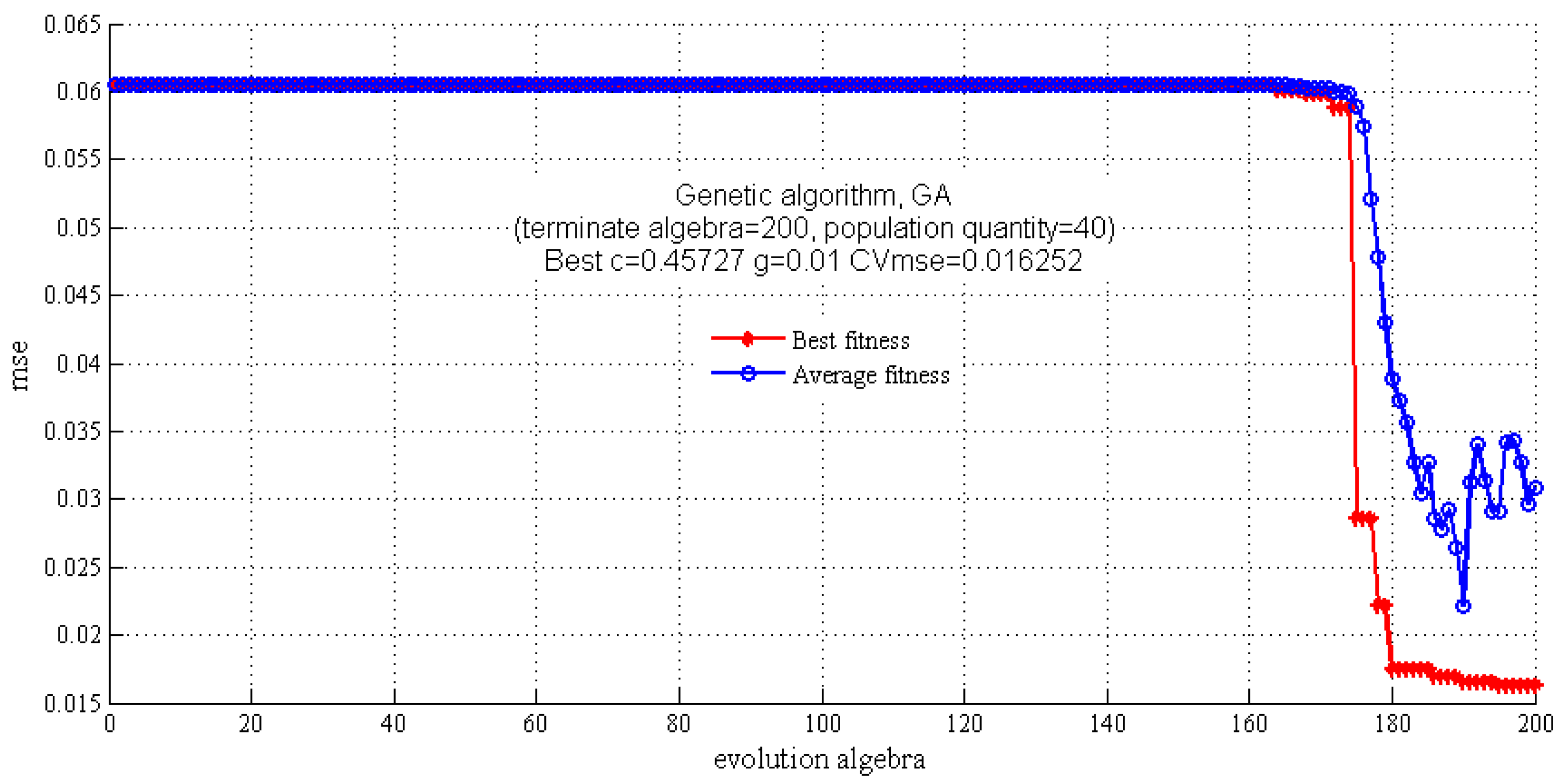
Figure 6.
The optimization results for parameters c and g by particle swarm optimization algorithm.

Figure 7.
Correlation diagram between FT-IR predicted values and the reference values in the training and validation sets for gentiopicroside.
Figure 7.
Correlation diagram between FT-IR predicted values and the reference values in the training and validation sets for gentiopicroside.


Table 1.
Statistics of the optimal calibration models.
| Types Parameter | Model 1 | Model 2 | Model 3 | Model 4 | |||||||||||
|---|---|---|---|---|---|---|---|---|---|---|---|---|---|---|---|
| Dali, Root | Diqing, Root | Lijiang, Root | Yuxi, Root | Dali, Stem | Diqing, Stem | Lijiang, Stem | Yuxi, Stem | Dali, Leaf | Diqing, Leaf | Lijiang, Leaf | Yuxi, Leaf | Root | Stem | Leaf | |
| R2 | 0.9543 | 0.9654 | 0.9426 | 0.9762 | 0.8346 | 0.8464 | 0.9098 | 0.9472 | 0.9031 | 0.8964 | 0.8854 | 0.9231 | 0.8334 | 0.8425 | 0.9331 |
| RMSEE | 0.0852 | 0.0985 | 0.1247 | 0.0615 | 0.1552 | 0.1999 | 0.1531 | 0.0877 | 0.1364 | 0.1695 | 0.1464 | 0.1140 | 0.1835 | 0.1927 | 0.1295 |
| RMSECV | 0.1785 | 0.2313 | 0.1992 | 0.0709 | 0.2740 | 0.2688 | 0.1807 | 0.1689 | 0.1614 | 0.1924 | 0.1680 | 0.1713 | 0.2272 | 0.2304 | 0.1445 |
Model evaluation statistics for partial least squares discriminant analysis (PLS-DA) models. R2: determination coefficient; RMSEE: root-mean-square error of estimation; RMSECV: root-mean-square error of cross-validation.
Table 2.
Results of the PLS-DA model 1 validation set samples.
| Samples | Actual Class | Calculated Class | YPre | Ydev |
|---|---|---|---|---|
| 2 | Dali, Root | Dali, Root | 1.1112 | 0.4306 |
| 4 | Dali, Root | Uncertain | 1.5243 | 0.6372 |
| 6 | Dali, Root | Uncertain | 1.5774 | 0.6637 |
| 7 | Dali, Root | Dali, Root | 1.2030 | 0.4765 |
| 13 | Lijiang, Root | Diqing, Root | 0.4190 | 0.1300 |
| 14 | Lijiang, Root | Lijiang, Root | 0.6108 | 0.2930 |
| 18 | Lijiang, Root | Lijiang, Root | 0.8904 | 0.3202 |
| 20 | Lijiang, Root | Lijiang, Root | 0.8029 | 0.3449 |
| 21 | Lijiang, Root | Lijiang, Root | 1.1986 | 0.4743 |
| 24 | Lijiang, Root | Lijiang, Root | 1.0592 | 0.4046 |
| 25 | Lijiang, Root | Lijiang, Root | 0.8340 | 0.2920 |
| 31 | Diqing, Root | Diqing, Root | 0.7014 | 0.2522 |
| 40 | Diqing, Root | Diqing, Root | 0.8934 | 0.3217 |
| 42 | Diqing, Root | Diqing, Root | 0.7153 | 0.2364 |
| 44 | Diqing, Root | Diqing, Root | 0.7702 | 0.2601 |
| 45 | Diqing, Root | Diqing, Root | 1.0444 | 0.3972 |
| 47 | Diqing, Root | Diqing, Root | 0.8626 | 0.3079 |
| 54 | Yuxi, Root | Yuxi-Root | 0.9195 | 0.3351 |
| 57 | Yuxi, Root | Uncertain | 1.3332 | 0.5416 |
| 59 | Yuxi, Root | Yuxi-Root | 1.1181 | 0.4341 |
Ypre: predicted value; Ydev and deviation values.
Table 3.
Results of the PLS-DA model 2 validation set samples.
| Samples | Actual Class | Calculated Class | YPre | Ydev |
|---|---|---|---|---|
| 61 | Dali, Stem | Dali, Stem | 0.9741 | 0.4110 |
| 62 | Dali, Stem | Dali, Stem | 1.1943 | 0.4722 |
| 66 | Dali, Stem | Dali, Stem | 0.8053 | 0.2776 |
| 70 | Dali, Stem | Dali, Stem | 0.5274 | 0.1387 |
| 72 | Lijiang, Stem | Lijiang, Stem | 1.0518 | 0.4318 |
| 74 | Lijiang, Stem | Lijiang, Stem | 0.9547 | 0.3524 |
| 76 | Lijiang, Stem | Uncertain | 1.3367 | 0.6355 |
| 81 | Lijiang, Stem | Lijiang, Stem | 0.7931 | 0.2796 |
| 87 | Lijiang, Stem | Lijiang, Stem | 1.0656 | 0.4078 |
| 88 | Lijiang, Stem | Lijiang, Stem | 1.0032 | 0.3766 |
| 91 | Diqing, Stem | Diqing, Stem | 1.2258 | 0.4879 |
| 94 | Diqing, Stem | Diqing, Stem | 1.1724 | 0.4612 |
| 95 | Diqing, Stem | Diqing, Stem | 1.0654 | 0.4077 |
| 104 | Diqing, Stem | Lijiang, Stem | 0.4763 | 0.2348 |
| 105 | Diqing, Stem | Diqing, Stem | 0.6590 | 0.2045 |
| 107 | Diqing, Stem | Lijiang, Stem | 0.3148 | 0.2175 |
| 112 | Yuxi, Stem | Yuxi, Stem | 0.9311 | 0.3704 |
| 117 | Yuxi, Stem | Yuxi, Stem | 0.9702 | 0.3601 |
| 120 | Yuxi, Stem | Yuxi, Stem | 0.9334 | 0.3417 |
Ypre: predicted value; Ydev and deviation values.
Table 4.
Results of PLS-DA model 3 validate set samples.
| Samples | Actual Class | Calculated Class | YPre | Ydev |
|---|---|---|---|---|
| 123 | Dali, Leaf | Dali, Leaf | 0.7455 | 0.2478 |
| 128 | Dali, Leaf | Uncertain | 1.4334 | 0.5917 |
| 133 | Lijiang, Leaf | Lijiang, Leaf | 0.8984 | 0.3242 |
| 134 | Lijiang, Leaf | Lijiang, Leaf | 0.6928 | 0.2214 |
| 135 | Lijiang, Leaf | Lijiang, Leaf | 0.5073 | 0.1949 |
| 136 | Lijiang, Leaf | Lijiang, Leaf | 0.8768 | 0.3134 |
| 137 | Lijiang, Leaf | Uncertain | 1.1790 | 0.6497 |
| 139 | Lijiang, Leaf | Lijiang, Leaf | 0.9106 | 0.3494 |
| 140 | Lijiang, Leaf | Lijiang, Leaf | 0.5083 | 0.1241 |
| 141 | Lijiang, Leaf | Lijiang, Leaf | 0.9160 | 0.3330 |
| 144 | Lijiang, Leaf | Lijiang, Leaf | 1.0707 | 0.4103 |
| 145 | Lijiang, Leaf | Lijiang, Leaf | 1.3312 | 0.5406 |
| 146 | Lijiang, Leaf | Dali, Leaf | 0.3026 | 0.1056 |
| 154 | Diqing, Leaf | Diqing, Leaf | 1.1157 | 0.4329 |
| 160 | Diqing, Leaf | Diqing, Leaf | 0.8556 | 0.3242 |
| 165 | Diqing, Leaf | Diqing, Leaf | 0.5760 | 0.1630 |
| 166 | Diqing, Leaf | Diqing, Leaf | 1.1611 | 0.4555 |
| 170 | Yuxi, Leaf | Yuxi, Leaf | 0.9046 | 0.3273 |
| 176 | Yuxi, Leaf | Yuxi, Leaf | 0.8712 | 0.3127 |
| 178 | Yuxi, Leaf | Yuxi, Leaf | 0.9259 | 0.3379 |
Ypre: predicted value; Ydev and deviation values.
Table 5.
Results of PLS-DA model 4 validation set samples.
| Samples | Actual Class | Calculated Class | YPre | Ydev |
|---|---|---|---|---|
| 5 | Root | Root | 0.7803 | 0.3378 |
| 6 | Root | Root | 0.9955 | 0.4414 |
| 7 | Root | Root | 0.7524 | 0.2794 |
| 12 | Root | Root | 0.9642 | 0.4205 |
| 13 | Root | Root | 0.9584 | 0.4167 |
| 14 | Root | Root | 0.8682 | 0.3566 |
| 15 | Root | Root | 0.7034 | 0.2467 |
| 18 | Root | Root | 0.8453 | 0.3500 |
| 19 | Root | Root | 0.8823 | 0.3660 |
| 20 | Root | Root | 0.8876 | 0.3695 |
| 21 | Root | Root | 0.6858 | 0.2350 |
| 22 | Root | Root | 0.8692 | 0.3573 |
| 24 | Root | Root | 0.9851 | 0.4345 |
| 29 | Root | Uncertain | 1.1444 | 0.5407 |
| 30 | Root | Root | 0.9511 | 0.4118 |
| 31 | Root | Root | 0.6869 | 0.2357 |
| 32 | Root | Root | 0.9623 | 0.4193 |
| 34 | Root | Root | 0.8161 | 0.3218 |
| 38 | Root | Root | 0.9635 | 0.4201 |
| 40 | Root | Root | 1.0701 | 0.4912 |
| 41 | Root | Root | 0.6536 | 0.2135 |
| 43 | Root | Root | 0.7605 | 0.2848 |
| 49 | Root | Root | 0.9819 | 0.4324 |
| 50 | Root | Root | 0.7037 | 0.3252 |
| 51 | Root | Uncertain | 1.2548 | 0.6143 |
| 52 | Root | Root | 0.9847 | 0.4343 |
| 53 | Root | Root | 0.8527 | 0.3462 |
| 57 | Root | Root | 0.8420 | 0.3391 |
| 58 | Stem | Stem | 0.5076 | 0.1588 |
| 61 | Stem | Uncertain | 1.1209 | 0.5250 |
| 62 | Stem | Uncertain | 1.2384 | 0.6033 |
| 63 | Stem | Root | 0.2768 | 0.2470 |
| 70 | Stem | Stem | 0.6177 | 0.1896 |
| 71 | Stem | Stem | 0.7688 | 0.2903 |
| 73 | Stem | Stem | 0.6066 | 0.1822 |
| 78 | Stem | Root | 0.1209 | 0.2604 |
| 82 | Stem | Stem | 0.7153 | 0.2596 |
| 83 | Stem | Root | 0.4597 | 0.0842 |
| 84 | Stem | Stem | 0.6782 | 0.2299 |
| 86 | Stem | Stem | 1.0495 | 0.4932 |
| 89 | Stem | Stem | 0.7826 | 0.2995 |
| 104 | Stem | Stem | 0.7306 | 0.2648 |
| 106 | Stem | Uncertain | 1.2252 | 0.5946 |
| 108 | Stem | Stem | 0.8728 | 0.3596 |
| 110 | Stem | Stem | 0.7044 | 0.2639 |
| 111 | Stem | Uncertain | 1.5978 | 0.8430 |
| 112 | Stem | Stem | 1.0158 | 0.4550 |
| 122 | Leaf | Leaf | 1.0092 | 0.4505 |
| 123 | Leaf | Leaf | 0.9702 | 0.4246 |
| 129 | Leaf | Leaf | 0.6900 | 0.2377 |
| 130 | Leaf | Leaf | 0.9760 | 0.4285 |
| 132 | Leaf | Leaf | 0.7933 | 0.3066 |
| 133 | Leaf | Leaf | 0.8667 | 0.3556 |
| 141 | Leaf | Leaf | 0.8623 | 0.3526 |
| 149 | Leaf | Leaf | 0.9041 | 0.3805 |
| 153 | Leaf | Leaf | 0.9990 | 0.4438 |
| 159 | Leaf | Leaf | 0.8485 | 0.3434 |
| 163 | Leaf | Leaf | 0.9792 | 0.4325 |
| 165 | Leaf | Leaf | 1.0081 | 0.4499 |
| 170 | Leaf | Leaf | 0.9311 | 0.3985 |
Ypre: predicted value; Ydev and deviation values.
Table 6.
Statistics of the SVM models.
| Model | c | g | CVmse | Rt2 (%) | RMSEE | Rv2 (%) | RMSEP |
|---|---|---|---|---|---|---|---|
| GS-SVM | 0.5000 | 0.0040 | 0.0149 | 92.7143 | 3.1056 | 83.5721 | 11.1421 |
| GA-SVM | 0.4573 | 0.0100 | 0.0163 | 96.3977 | 3.1760 | 82.3279 | 11.1504 |
| PSO-SVM | 0.4454 | 0.0100 | 0.0162 | 96.3120 | 3.2131 | 82.3529 | 11.1506 |
Rt2: determination coefficient for training set; Rv2: determination coefficient for validated set; RMSEE: root-mean-square error of estimation; RMSEP: root-mean-square error of prediction.
Table 7.
Information of G. rigescens.
| No. | Site | Description | No. | Site | Description | No. | Site | Description |
|---|---|---|---|---|---|---|---|---|
| 1–10 | Dali, Yunnan | Root | 61–70 | Dali, Yunnan | Stem | 121–130 | Dali, Yunnan | Leaf |
| 11–30 | Lijiang, Yunnan | Root | 71–90 | Lijiang, Yunnan | Stem | 131–149 | Lijiang, Yunnan | Leaf |
| 31–50 | Diqing, Yunnan | Root | 91–110 | Diqing, Yunnan | Stem | 150–169 | Diqing, Yunnan | Leaf |
| 51–60 | Yuxi, Yunnan | Root | 111–120 | Yuxi, Yunnan | Stem | 170–179 | Yuxi, Yunnan | Leaf |
© 2017 by the authors. Licensee MDPI, Basel, Switzerland. This article is an open access article distributed under the terms and conditions of the Creative Commons Attribution (CC BY) license (http://creativecommons.org/licenses/by/4.0/).
Share and Cite
MDPI and ACS Style
Wu, Z.; Zhao, Y.; Zhang, J.; Wang, Y. Quality Assessment of Gentiana rigescens from Different Geographical Origins Using FT-IR Spectroscopy Combined with HPLC. Molecules 2017, 22, 1238. https://doi.org/10.3390/molecules22071238
AMA Style
Wu Z, Zhao Y, Zhang J, Wang Y. Quality Assessment of Gentiana rigescens from Different Geographical Origins Using FT-IR Spectroscopy Combined with HPLC. Molecules. 2017; 22(7):1238. https://doi.org/10.3390/molecules22071238
Chicago/Turabian StyleWu, Zhe, Yanli Zhao, Ji Zhang, and Yuanzhong Wang. 2017. "Quality Assessment of Gentiana rigescens from Different Geographical Origins Using FT-IR Spectroscopy Combined with HPLC" Molecules 22, no. 7: 1238. https://doi.org/10.3390/molecules22071238