Behavior of the E–E’ Bonds (E, E’ = S and Se) in Glutathione Disulfide and Derivatives Elucidated by Quantum Chemical Calculations with the Quantum Theory of Atoms-in-Molecules Approach


Abstract
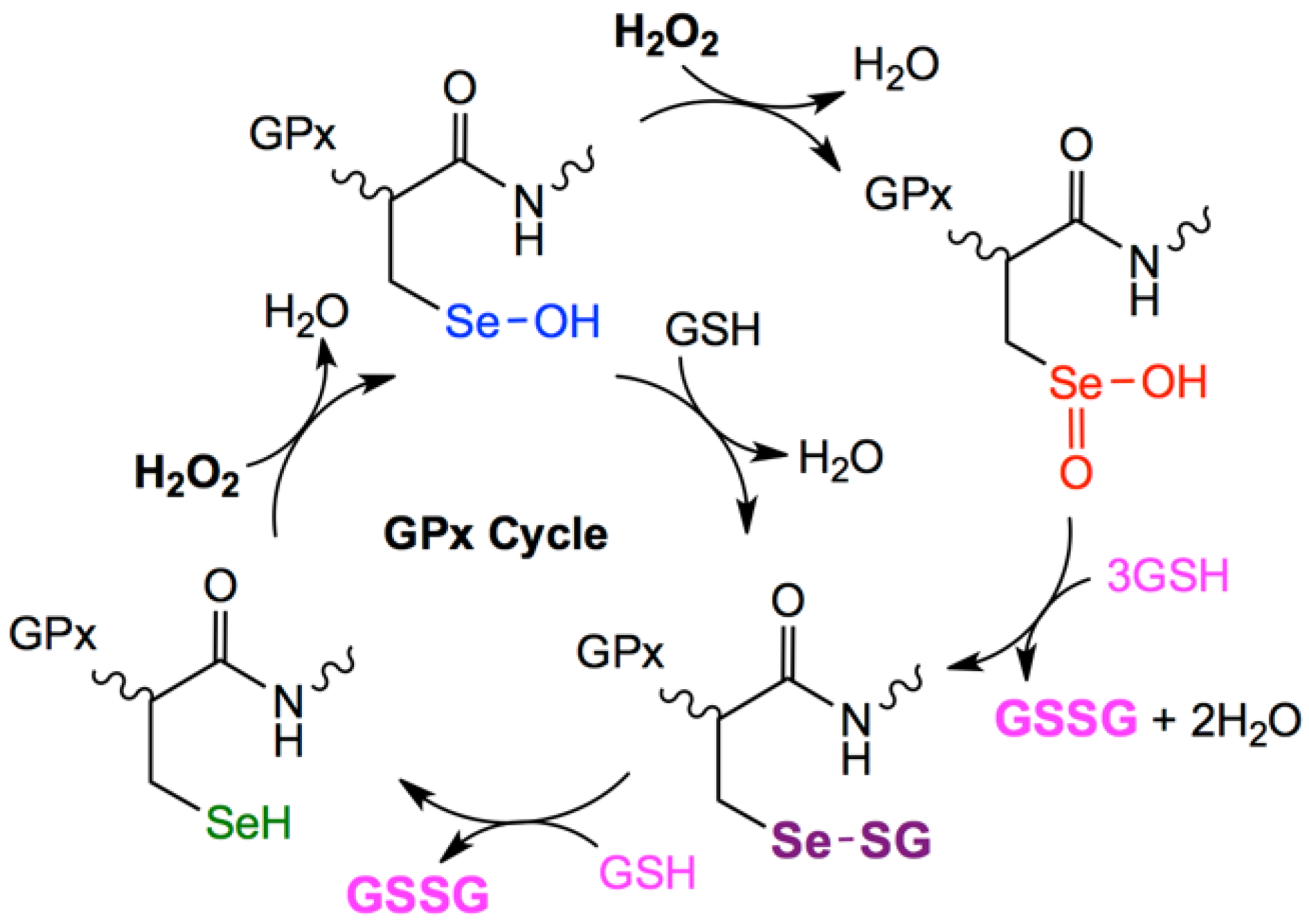
:1. Introduction
2. Methodological Details in Calculations
3. Results and Discussion
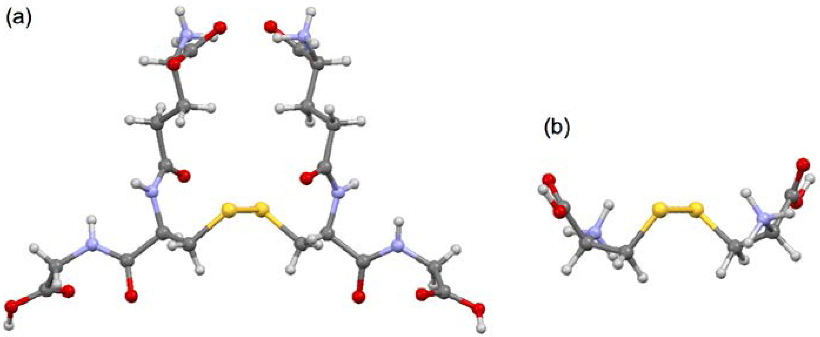
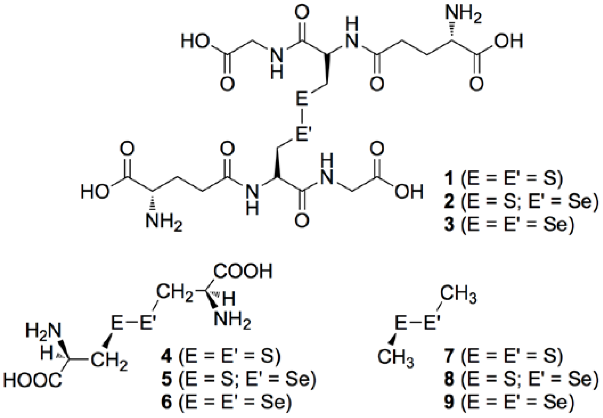
3.1. Optimized Structures for Conformers of 1–6 with M06-2X/BSS-A, Together with 7–9
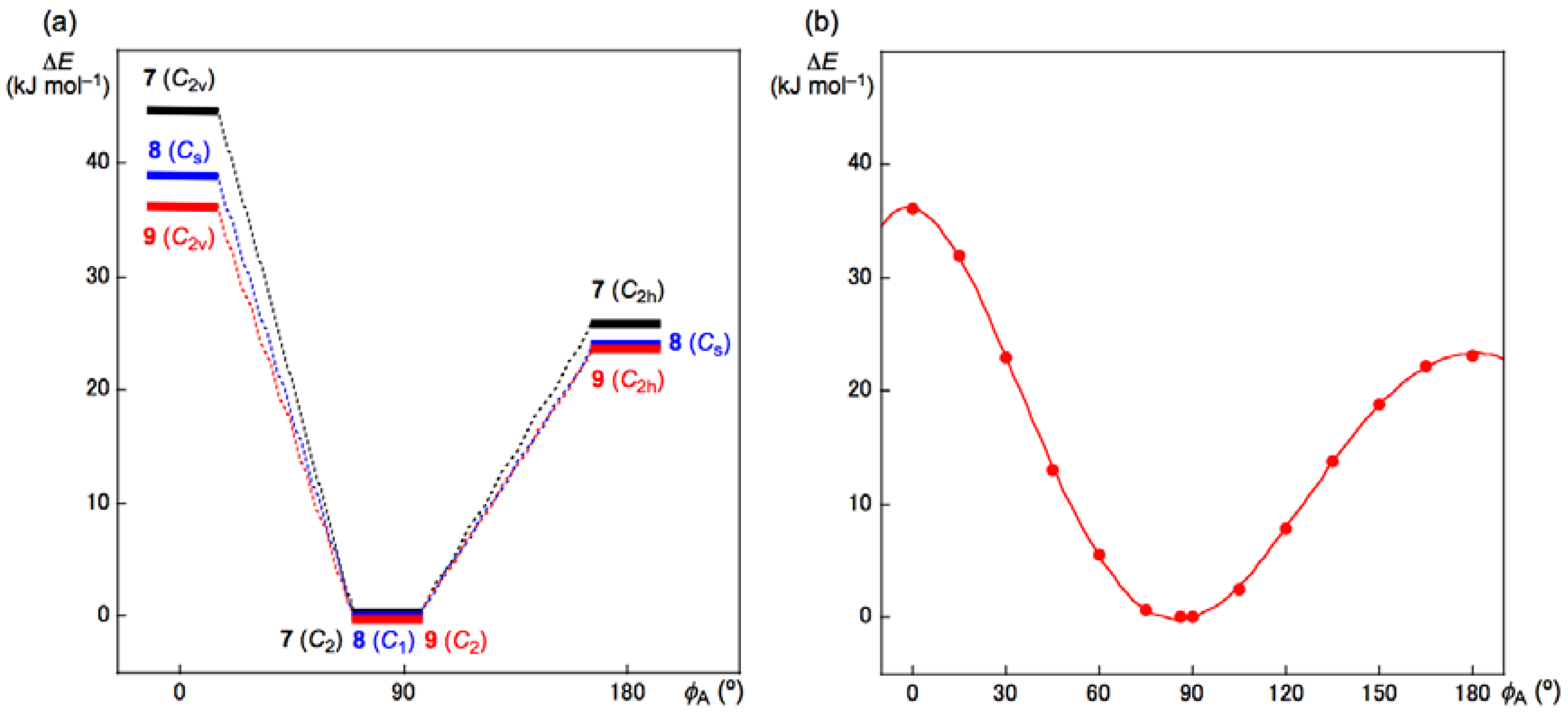
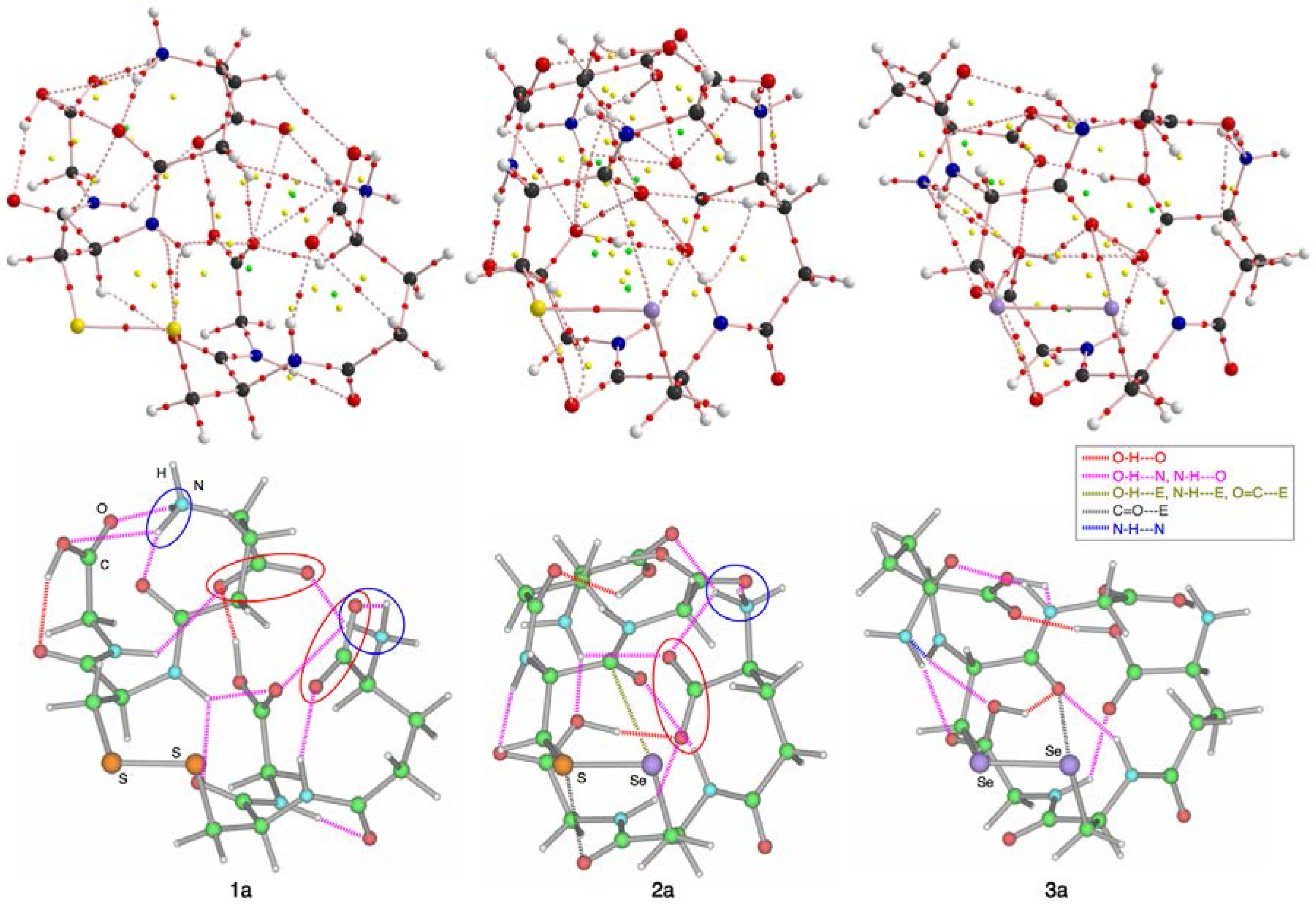
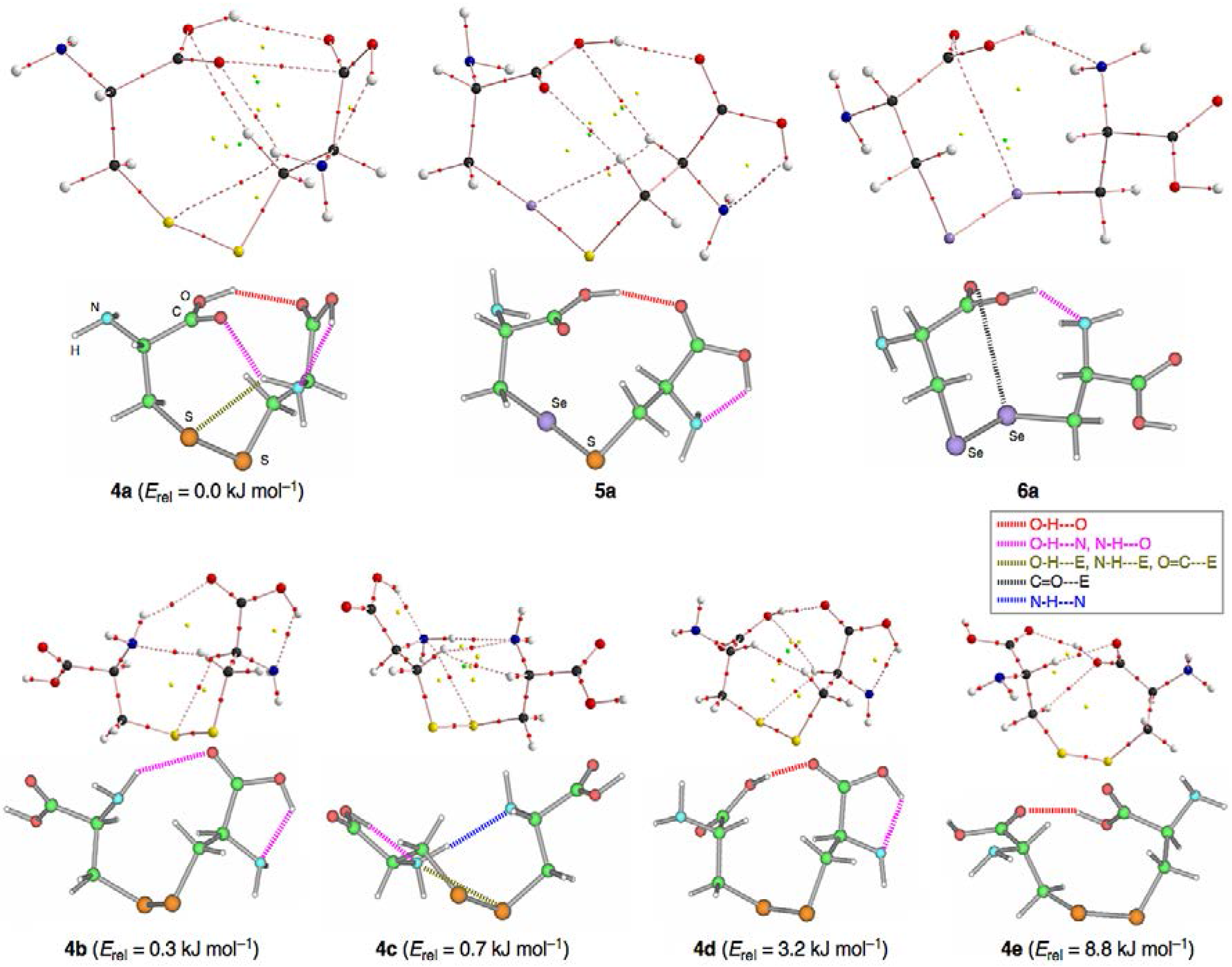
3.2. Structural Feature of 1a–6a and 7–9
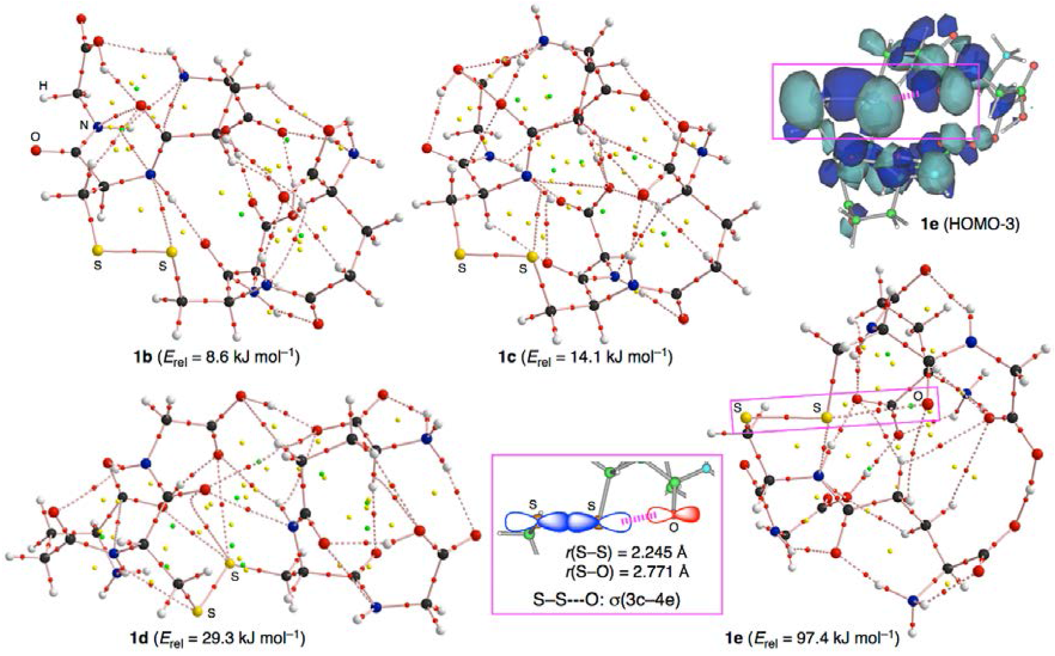
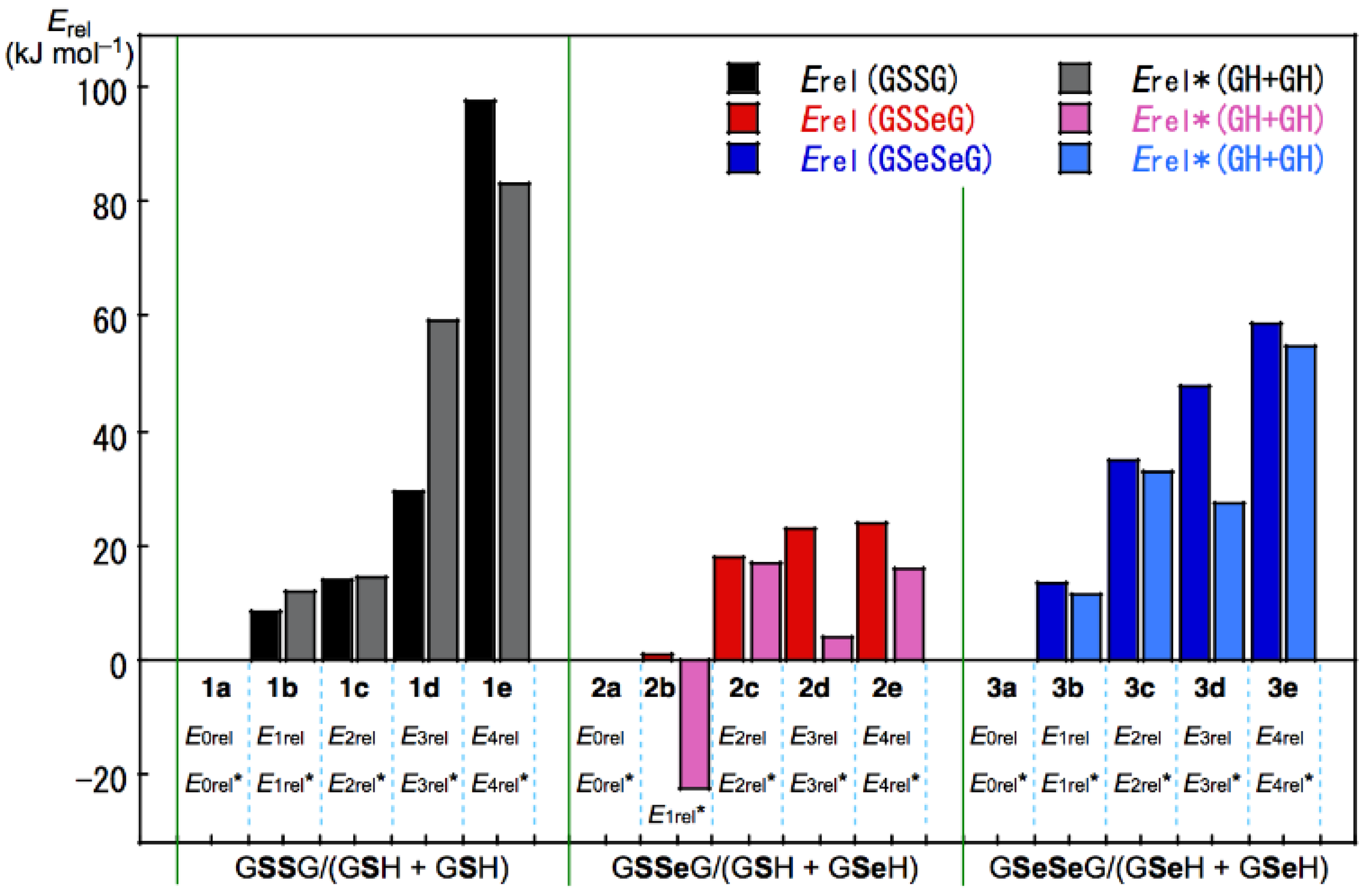
3.3. Factors Determining the Relative Energies of 1a–6a
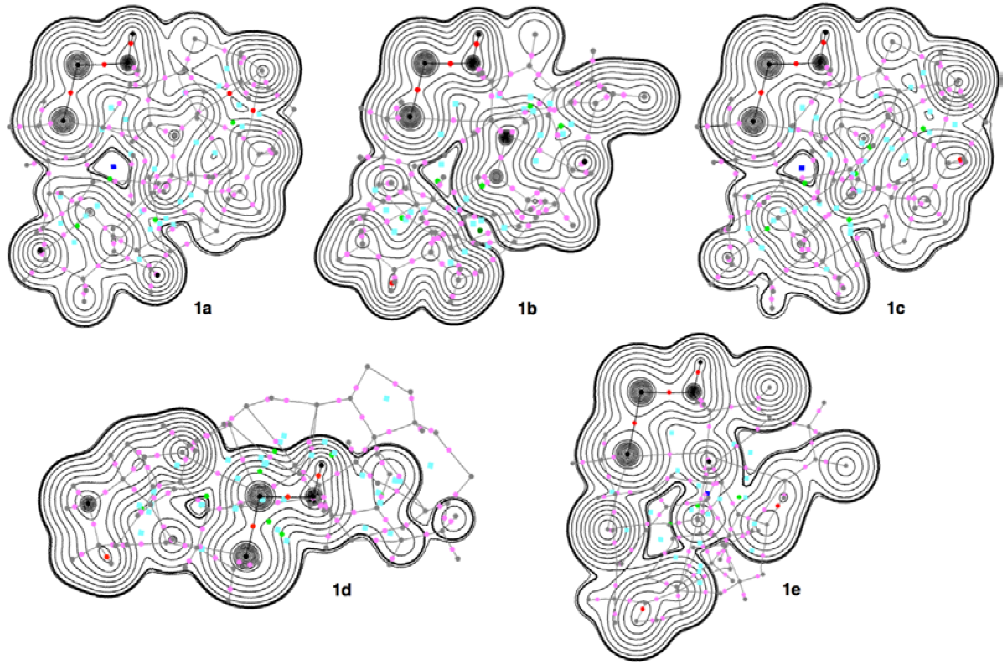
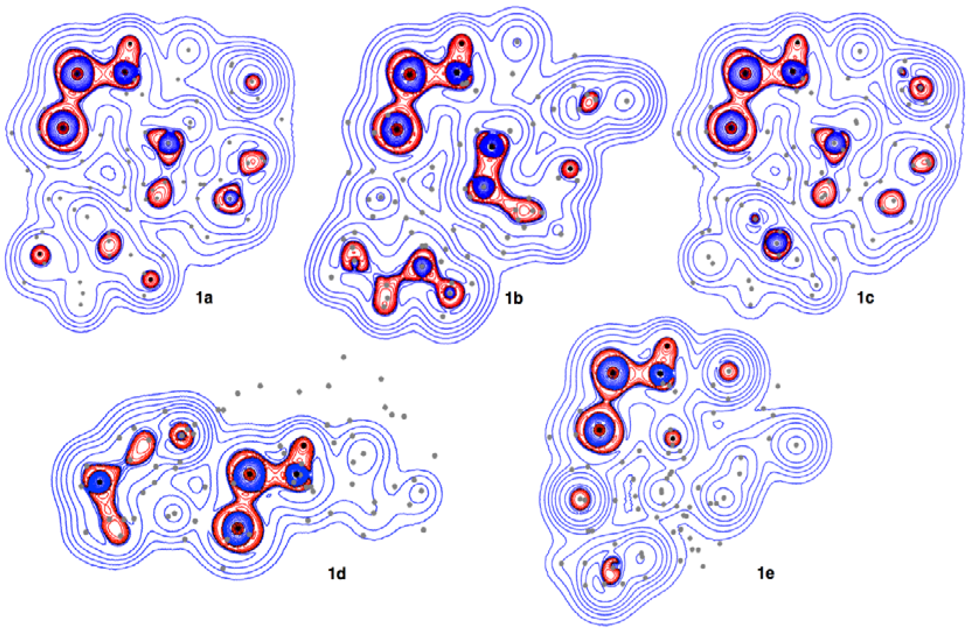
3.4. Contour Plots and Negative Laplacian around the E-∗-E’ Bonds in 1a–6e
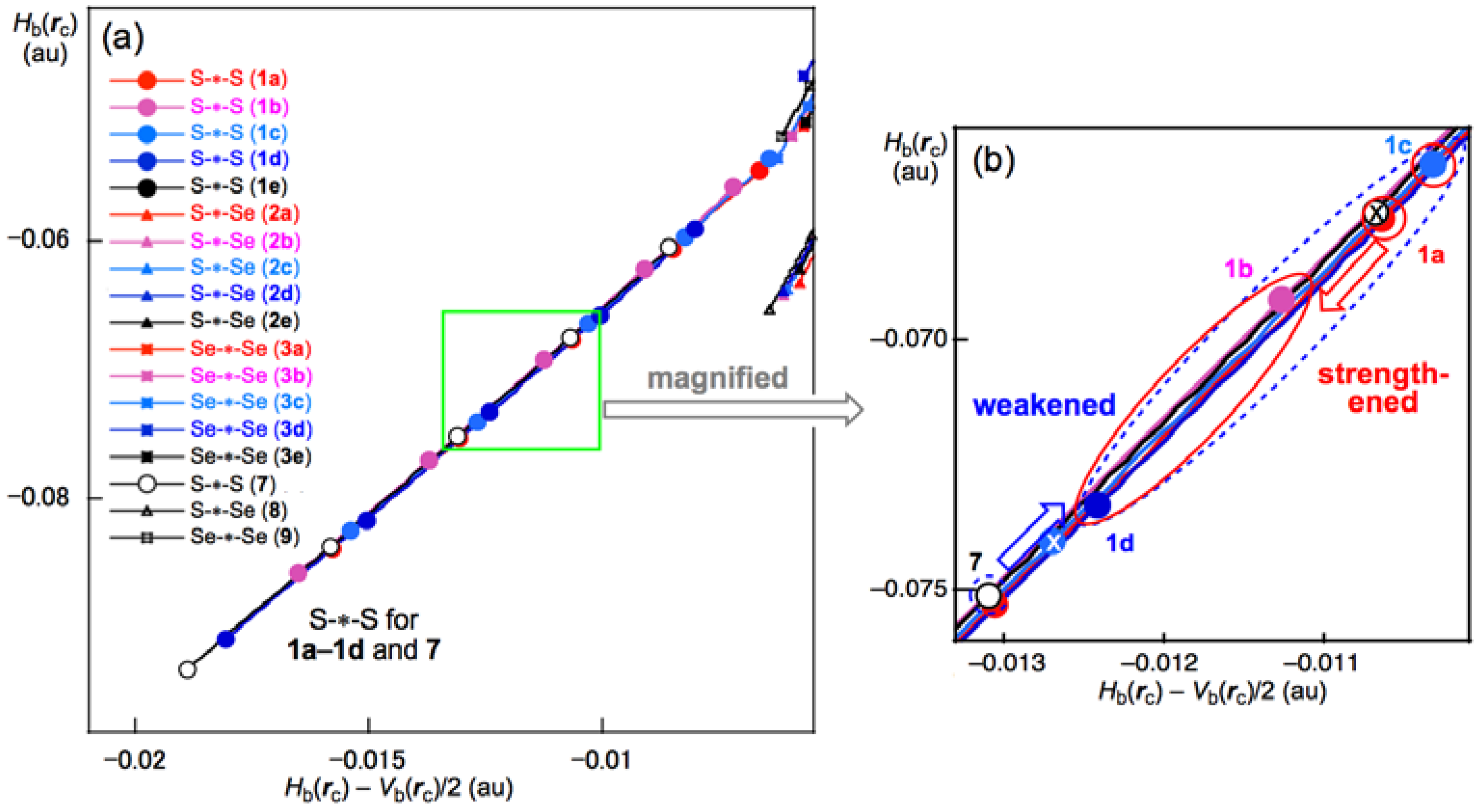
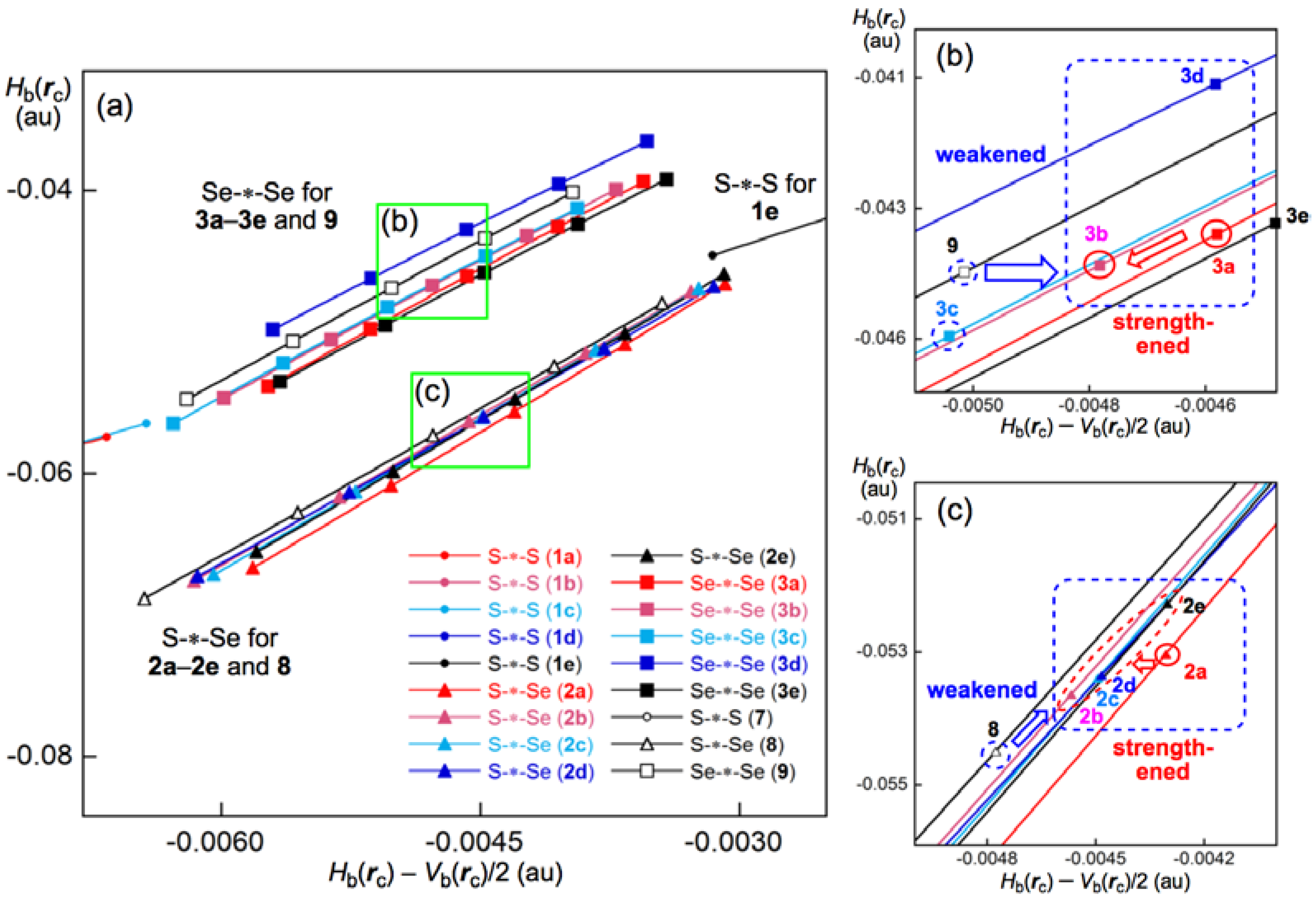
3.5. Application of QTAIM-DFA to the E–E’ Bonds in 1a–6e
3.6. Nature of the E–E’ Bonds in 1a–6e
3.7. Factors that Stabilize the E–E’ Bonds and the Conformers
4. Conclusions
Supplementary Materials
Acknowledgments
Author Contributions
Conflicts of Interest
References and Notes
- Nakanishi, W.; Hayashi, S.; Morinaka, S.; Sasamori, T.; Tokitoh, N. Extended hypervalent E’···E–E···E’ 4c–6e (E, E’ = Se, S) interactions: Structure, stability and reactivity of 1-(8-PhE’C10H6)EE(C10H6E’Ph-8’)-1’. New J. Chem. 2008, 32, 1881–1889. [Google Scholar] [CrossRef]
- Hwang, C.; Sinskey, A.J.; Lodish, H.F. Oxidized redox state of glutathione in the endoplasmic reticulum. Science 1992, 257, 1496–1502. [Google Scholar] [CrossRef] [PubMed]
- Wetlaufer, D.B.; Branca, P.A.; Chen, G.-X. The oxidative folding of proteins by disulfide plus thiol does not correlate with redox potential. Protein Eng. 1987, 1, 141–146. [Google Scholar] [CrossRef] [PubMed]
- Gilbert, H.F. Thiol/disulfide exchange equilibria and disulfidebond stability. Methods Enzymol. 1995, 251, 8–28. [Google Scholar] [PubMed]
- Lyles, M.M.; Gilbert, H.F. Catalysis of the oxidative folding of ribonuclease A by protein disulfide isomerase: Dependence of the rate on the composition of the redox buffer. Biochemistry 1991, 30, 613–619. [Google Scholar] [CrossRef] [PubMed]
- Beld, J.; Kenneth, W.J.; Hilvert, D. Selenoglutathione: Efficient Oxidative Protein Folding by a Diselenide. Biochemistry 2007, 46, 5382–5390. [Google Scholar] [CrossRef] [PubMed]
- Konishi, Y.; Ooi, T.; Scheraga, H.A. Regeneration of ribonuclease A from the reduced protein. 1. Rate-limiting steps. Biochemistry 1982, 21, 4734–4740. [Google Scholar] [CrossRef] [PubMed]
- Hendrickson, W.A. Determination of macromolecular structures from anomalous diffraction of synchrotron radiation. Science 1991, 254, 51–58. [Google Scholar] [CrossRef] [PubMed]
- See references cited in [18].
- Kumakura, F.; Mishra, B.; Priyadarsini, K.I.; Iwaoka, M. A Water-Soluble Cyclic Selenide with Enhanced Glutathione Peroxidase-Like Catalytic Activities. Eur. J. Org. Chem. 2010, 440–445. [Google Scholar] [CrossRef]
- Arai, K.; Dedachi, K.; Iwaoka, M. Rapid and Quantitative Disulfide Bond Formation for a Polypeptide Chain Using a Cyclic Selenoxide Reagent in an Aqueous Medium. Chem. Eur. J. 2011, 17, 481–485. [Google Scholar] [CrossRef] [PubMed]
- Yoshida, S.; Kumakura, F.; Komatsu, I.; Arai, K.; Onuma, Y.; Hojo, H.; Singh, B.G.; Priyadarsini, K.I.; Iwaoka, M. Antioxidative Glutathione Peroxidase Activity of Selenoglutathione. Angew. Chem. Int. Ed. 2011, 50, 2125–2128. [Google Scholar] [CrossRef] [PubMed]
- Manna, D.; Mugesh, G. Regioselective Deiodination of Thyroxine by Iodothyronine Deiodinase Mimics: An Unusual Mechanistic Pathway Involving Cooperative Chalcogen and Halogen Bonding. J. Am. Chem. Soc. 2012, 134, 4269–4279. [Google Scholar] [CrossRef] [PubMed]
- Flohe, L.; Günzler, W.A.; Schock, H.H. Glutathione peroxidase: A selenoenzyme. FEBS Lett. 1973, 32, 132–134. [Google Scholar] [CrossRef]
- Flohe, L. Glutathione Peroxidase Brought into Focus. Free Radic. Biol. 1982, 5, 223–254. [Google Scholar]
- Jelsch, C.; Didierjean, C. The oxidized form of glutathione. Acta Cryst. C 1999, 55, 1538–1540, CSD code: BERLOZ. [Google Scholar] [CrossRef]
- Leela, S.; Ramamurthi, K. Private Communication, 2007. CSD code: CYSTCL03.
- Tsubomoto, Y.; Hayashi, S.; Nakanishi, W. Dynamic and static behavior of the E–E’ bonds (E, E’ = S and Se) in cystine and derivatives, elucidated by AIM dual functional analysis. RSC Adv. 2015, 5, 11534–11540. [Google Scholar] [CrossRef]
- Bader, R.F.W. Atoms in Molecules. A Quantum Theory; Oxford University Press: Oxford, UK, 1990. [Google Scholar]
- Matta, C.F.; Boyd, R.J. An Introduction to the Quantum Theory of Atoms in Molecules in the Quantum Theory of Atoms in Molecules: From Solid State to DNA and Drug Design; WILEY-VCH: Weinheim, Germany, 2007. [Google Scholar]
- Biegler-König, F.; Schönbohm, J. Update of the AIM2000-Program for atoms in molecules. J. Comput. Chem. 2002, 23, 1489–1494. [Google Scholar] [CrossRef] [PubMed]
- Biegler-König, F.; Schönbohm, J.; Bayles, D. AIM2000. J. Comput. Chem. 2001, 22, 545–559. [Google Scholar]
- Bader, R.F.W. A Bond Path: A Universal Indicator of Bonded Interactions. J. Phys. Chem. A 1998, 102, 7314–7323. [Google Scholar] [CrossRef]
- Bader, R.F.W. A quantum theory of molecular structure and its applications. Chem. Rev. 1991, 91, 893–926. [Google Scholar] [CrossRef]
- Bader, R.F.W. Atoms in molecules. Acc. Chem. Res. 1985, 18, 9–15. [Google Scholar] [CrossRef]
- Tang, T.H.; Bader, R.F.W.; MacDougall, P. Structure and bonding in sulfur-nitrogen compounds. Inorg. Chem. 1985, 24, 2047–2053. [Google Scholar] [CrossRef]
- Bader, R.F.W.; Slee, T.S.; Cremer, D.; Kraka, E. Description of conjugation and hyperconjugation in terms of electron distributions. J. Am. Chem. Soc. 1983, 105, 5061–5068. [Google Scholar] [CrossRef]
- Biegler-König, F.; Bader, R.F.W.; Tang, T.H. Calculation of the average properties of atoms in molecules. J. Comput. Chem. 1982, 3, 317–328. [Google Scholar] [CrossRef]
- Bader, R.F.W. Bond Paths Are Not Chemical Bonds. J. Phys. Chem. A 2009, 113, 10391–10396. [Google Scholar] [CrossRef] [PubMed]
- Foroutan-Nejad, C.; Shahbazian, S.; Marek, R. Toward a Consistent Interpretation of the QTAIM: Tortuous Link between Chemical Bonds, Interactions, and Bond/Line Paths. Chem. Eur. J. 2014, 20, 10140–10152. [Google Scholar] [CrossRef] [PubMed]
- Garcıa-Revilla, M.; Francisco, E.; Popelier, P.L.A.; Pendás, A.M. Domain-Averaged Exchange-Correlation Energies as a Physical Underpinning for Chemical Graphs. ChemPhysChem 2013, 14, 1211–1218. [Google Scholar] [CrossRef] [PubMed]
- Keyvani, Z.A.; Shahbazian, S.; Zahedi, M. To What Extent are “Atoms in Molecules” Structures of Hydrocarbons Reproducible from the Promolecule Electron Densities? Chem. Eur. J. 2016, 22, 5003–5009. [Google Scholar] [CrossRef] [PubMed]
- Poater, J.; Sol, M.; Bickelhaupt, F.M. Hydrogen–Hydrogen Bonding in Planar Biphenyl, Predicted by Atoms-In-Molecules Theory, Does Not Exist. Chem. Eur. J. 2006, 12, 2889–2895. [Google Scholar] [CrossRef] [PubMed]
- Shahbazian, S. Why Bond Critical Points Are Not “Bond” Critical Points. Chem. Eur. J. 2018. [Google Scholar] [CrossRef] [PubMed]
- Nakanishi, W.; Hayashi, S.; Narahara, K. Polar Coordinate Representation of Hb(rc) versus (ћ2/8m)∇2ρb(rc) at BCP in AIM Analysis: Classification and Evaluation of Weak to Strong Interactions. J. Phys. Chem. A 2009, 113, 10050–10057. [Google Scholar] [CrossRef] [PubMed]
- Nakanishi, W.; Hayashi, S. Atoms-in-Molecules Dual Parameter Analysis of Weak to Strong Interactions: Behaviors of Electronic Energy Densities versus Laplacian of Electron Densities at Bond Critical Points. J. Phys. Chem. A 2008, 112, 13593–13599. [Google Scholar] [CrossRef] [PubMed]
- Nakanishi, W.; Hayashi, S. Atoms-in-Molecules Dual Functional Analysis of Weak to Strong Interactions. Curr. Org. Chem. 2010, 14, 181–197. [Google Scholar] [CrossRef]
- Nakanishi, W.; Hayashi, S. Dynamic Behaviors of Interactions: Application of Normal Coordinates of Internal Vibrations to AIM Dual Functional Analysis. J. Phys. Chem. A 2010, 114, 7423–7430. [Google Scholar] [CrossRef] [PubMed]
- Nakanishi, W.; Hayashi, S.; Matsuiwa, K.; Kitamoto, M. Applications of Normal Coordinates of Internal Vibrations to Generate Perturbed Structures: Dynamic Behavior of Weak to Strong Interactions Elucidated by Atoms-in-Molecules Dual Functional Analysis. Bull. Chem. Soc. Jpn. 2012, 85, 1293–1305. [Google Scholar] [CrossRef]
- QTAIM-DFA is successfully applied to analyze weak to strong interactions in gas phase. It could also be applied to the interactions in crystals and to those in larger systems, containing bioactive materials, the methodological improvement is inevitable to generate the perturbed structures suitable for the systems.
- Hayashi, S.; Matsuiwa, K.; Kitamoto, M.; Nakanishi, W. Dynamic Behavior of Hydrogen Bonds from Pure Closed Shell to Shared Shell Interaction Regions Elucidated by AIM Dual Functional Analysis. J. Phys. Chem. A 2013, 117, 1804–1816. [Google Scholar] [CrossRef] [PubMed]
- Sugibayashi, Y.; Hayashi, S.; Nakanishi, W. Dynamic and static behavior of hydrogen bonds of the X–H···π type (X = F, Cl, Br, I, RO and RR’N; R, R’ = H or Me) in the benzene π-system, elucidated by QTAIM dual functional analysis. Phys. Chem. Chem. Phys. 2015, 17, 28879–28891. [Google Scholar] [CrossRef] [PubMed]
- Hayashi, S.; Sugibayashi, Y.; Nakanishi, W. Dynamic and static behavior of the H···π and E···π interactions in EH2 adducts of benzene π-system (E = O, S, Se and Te), elucidated by QTAIM dual functional analysis. Phys. Chem. Chem. Phys. 2016, 18, 9948–9960. [Google Scholar] [CrossRef] [PubMed]
- Hayashi, S.; Matsuiwa, K.; Nishizawa, N.; Nakanishi, W. Transannular E···E’ Interactions in Neutral, Radical Cationic, and Dicationic Forms of cyclo-[E(CH2CH2CH2)2E’] (E, E’ = S, Se, Te, and O) with Structural Feature: Dynamic and Static Behavior of E···E’ Elucidated by QTAIM Dual Functional Analysis. J. Org. Chem. 2015, 80, 11963–11976. [Google Scholar] [CrossRef] [PubMed]
- Sugibayashi, Y.; Hayashi, S.; Nakanishi, W. Behavior of Halogen Bonds of the Y–X···π Type (X, Y = F, Cl, Br, I) in the Benzene π System, Elucidated by Using a Quantum Theory of Atoms in Molecules Dual-Functional Analysis. Chem. Phys. Chem. 2016, 17, 2579–2589. [Google Scholar] [CrossRef] [PubMed]
- Frisch, M.J.; Trucks, G.W.; Schlegel, H.B.; Scuseria, G.E.; Robb, M.A.; Cheeseman, J.R.; Scalmani, G.; Barone, V.; Mennucci, B.; Petersson, G.A.; et al. Gaussian 09 (Revision D.01); Gaussian, Inc.: Wallingford, CT, USA, 2009. [Google Scholar]
- Binning, R.C.; Curtiss, L.A. Compact contracted basis sets for third-row atoms: Ga–Kr. J. Comput. Chem. 1990, 11, 1206–1216. [Google Scholar] [CrossRef]
- Curtiss, L.A.; McGrath, M.P.; Blaudeau, J.-P.; Davis, N.E.; Binning, R.C., Jr.; Radom, L. Extension of Gaussian-2 theory to molecules containing third-row atoms Ga–Kr. J. Chem. Phys. 1995, 103, 6104–6113. [Google Scholar] [CrossRef]
- McGrath, M.P.; Radom, L. Extension of Gaussian-1 (G1) theory to bromine-containing molecules. J. Chem. Phys. 1991, 94, 511–516. [Google Scholar] [CrossRef]
- Clark, T.; Chandrasekhar, J.; Spitznagel, G.W.; Schleyer, P.V.R. Efficient diffuse function-augmented basis sets for anion calculations. III. The 3-21+G basis set for first-row elements, Li–F. J. Comput. Chem. 1983, 4, 294–301. [Google Scholar] [CrossRef]
- Zhao, Y.; Truhlar, D.G. The M06 suite of density functionals for main group thermochemistry, thermochemical kinetics, noncovalent interactions, excited states, and transition elements: Two new functionals and systematic testing of four M06-class functionals and 12 other functionals. Theor. Chem. Acc. 2008, 120, 215–241. [Google Scholar]
- Spartan ’02 Windows, Tutorial and User’s Guide; Wavefunction, Inc.: Irvine, CA, USA, 2001.
- Halgren, T.A. Merck molecular force field. I. Basis, form, scope, parameterization, and performance of MMFF94. J. Comput. Chem. 1996, 17, 490–519. [Google Scholar] [CrossRef]
- Becke, A.D. Density-functional thermochemistry. III. The role of exact exchange. J. Chem. Phys. 1993, 98, 5648–5652. [Google Scholar] [CrossRef]
- Lee, C.; Yang, W.; Parr, R.G. Development of the Colle-Salvetti correlation-energy formula into a functional of the electron density. Phys. Rev. B 1988, 37, 785–789. [Google Scholar] [CrossRef]
- Stewart, J.J.P. Optimization of parameters for semiempirical methods I. Method. J. Comput. Chem. 1989, 10, 209–220. [Google Scholar] [CrossRef]
- Reed, A.E.; Curtiss, L.A.; Weinhold, F. Intermolecular interactions from a natural bond orbital, donor-acceptor viewpoint. Chem. Rev. 1988, 88, 899–926. [Google Scholar] [CrossRef]
- Glendening, E.D.; Landis, C.R.; Weinhold, F. NBO 6.0: Natural bond orbital analysis program. J. Compt. Chem. 2013, 34, 1429–1437. [Google Scholar] [CrossRef] [PubMed]
- The AIM2000 program (Version 2.0) is employed to analyze and visualize atoms-in-molecules: Biegler-König, F. Calculation of atomic integration data. J. Comput. Chem. 2000, 21, 1040–1048. [Google Scholar]see also refs 19 and 20
- The values of w = (0), ±0.1, and ±0.2 in r = ro + wao were employed for the perturbed structures in [33,34], which covers roughly the observed range of the interaction distances in molecular complexes. The bond orders become 2/3 and 3/2 times larger at w = +0.2 and –0.2, respectively, relative to the original values at w = 0. However, it seems better to employ the perturbed structures closer to the fully optimized one, which will reduce the calculation errors from the perturbed structures. Therefore, w = (0), ±0.05, and ±0.1 have been used for r = ro + wao in the usual cases of the CS interactions. The shorter range of w must be more suitable for the SS interactions, although w = (0), ±0.05, and ±0.1 are employed in this paper.
- Nakanishi, W.; Hayashi, S. Role of dG/dw and dV/dw in AIM Analysis: An Approach to the Nature of Weak to Strong Interactions. J. Phys. Chem. A 2013, 117, 1795–1803. [Google Scholar] [CrossRef] [PubMed]
- Nakanishi, W.; Hayashi, S.; Hashimoto, M.; Arca, M.; Aragoni, M.C.; Lippolis, V. Recent advances of structural chemistry of organoselenium and organotellurium compounds. In The Chemistry of Organic Selenium and Tellurium Compounds; Rappoport, Z., Ed.; Wiley: New York, NY, USA, 2013; Volume 4, Chapter 11; pp. 885–972. [Google Scholar]


| Species | r(E, E) | φA | Erel | Species | r(E, E) | φA | Erel |
|---|---|---|---|---|---|---|---|
| (Å) | (°) | (kJ mol−1) | (Å) | (°) | (kJ mol−1) | ||
| 1a | 2.0736 | −117.4 | 0.0 | 2a | 2.2002 | −85.6 | 0.0 |
| 1b | 2.0694 | −116.4 | 8.6 | 2b | 2.1963 | −110.1 | 1.0 |
| 1c | 2.0778 | −119.3 | 14.1 | 2c | 2.1982 | −84.5 | 18.0 |
| 1d | 2.0561 | 100.3 | 29.3 | 2d | 2.1959 | −78.4 | 23.1 |
| 1e | 2.2454 | 117.9 | 97.4 | 2e | 2.2079 | −65.0 | 23.7 |
| 4a | 2.0625 | 67.7 | 0.0 | 5a | 2.1984 | −83.9 | 0.0 |
| 4b | 2.0471 | −82.2 | 0.3 | 5b | 2.1890 | 84.3 | 15.7 |
| 4c | 2.0529 | 88.5 | 0.7 | 5c | 2.2011 | 94.0 | 17.5 |
| 4d | 2.0541 | −75.7 | 3.2 | 5d | 2.2070 | 72.9 | 19.6 |
| 4e | 2.0515 | 95.7 | 8.8 | 5e | 2.2067 | −66.9 | 27.4 |
| 7 | 2.0491 | 85.0 | 2 | 8 | 2.1923 | 85.6 | 2 |
| 3a | 2.3252 | −85.2 | 0.0 | ||||
| 3b | 2.3215 | −82.5 | 13.6 | ||||
| 3c | 2.3138 | −92.5 | 34.9 | ||||
| 3d | 2.3546 | −144.5 | 47.9 | ||||
| 3e | 2.3320 | 105.2 | 58.8 | ||||
| 6a | 2.3275 | 88.5 | 0.0 | ||||
| 6b | 2.3303 | 93.4 | 1.4 | ||||
| 6c | 2.3309 | 90.2 | 3.3 | ||||
| 6d | 2.3351 | 74.9 | 3.6 | ||||
| 6e | 2.3286 | 93.1 | 3.7 | ||||
| 9 | 2.3236 | 86.1 | 2 |
| Compound | ρ(rc) | c∇2ρb(rc) 2 | Hb(rc) | R 3 | θ 4 | kb(rc) 5 | νn 6 | kf 7 | θp:NIV 8 | κp:NIV 9 | Classification/ |
|---|---|---|---|---|---|---|---|---|---|---|---|
| (Sym: E-∗-E’) | (au) | (au) | (au) | (au) | (°) | (cm−1) | (mdyn Å−1) | (°) | (au−1) | Characterization | |
| 1a (C1: S-∗-S) | 0.1378 | −0.0106 | −0.0676 | 0.0684 | 188.9 | −2.460 | 493.3 | 0.928 | 197.3 | 0.82 | SS/Covweak |
| 1b (C1: S-∗-S) | 0.1391 | −0.0113 | −0.0692 | 0.0701 | 189.2 | −2.483 | 513.8 | 1.718 | 197.3 | 0.78 | SS/Covweak |
| 1c (C1: S-∗-S) | 0.1368 | −0.0103 | −0.0665 | 0.0673 | 188.8 | −2.451 | 489.7 | 0.910 | 197.2 | 0.84 | SS/Covweak |
| 1d (C1: S-∗-S) | 0.1428 | −0.0124 | −0.0733 | 0.0744 | 189.6 | −2.512 | 506.0 | 0.917 | 197.6 | 0.70 | SS/Covweak |
| 1e (C1: S-∗-S) | 0.1025 | −0.0011 | −0.0345 | 0.0345 | 181.9 | −2.070 | 353.7 | 0.447 | 193.8 | 3.62 | SS/Covweak |
| 2a (C1: S-∗-Se) | 0.1169 | −0.0043 | −0.0528 | 0.0530 | 184.7 | −2.195 | 418.7 | 0.545 | 188.1 | 0.23 | SS/Covweak |
| 2b (C1: S-∗-Se) | 0.1178 | −0.0046 | −0.0535 | 0.0537 | 184.9 | −2.206 | 434.0 | 0.955 | 188.4 | 0.15 | SS/Covweak |
| 2c (C1: S-∗-Se) | 0.1174 | −0.0045 | −0.0532 | 0.0534 | 184.8 | −2.203 | 421.5 | 0.634 | 188.3 | 0.19 | SS/Covweak |
| 2d (C1: S-∗-Se) | 0.1176 | −0.0045 | −0.0532 | 0.0534 | 184.8 | −2.203 | 404.6 | 0.684 | 188.7 | 0.21 | SS/Covweak |
| 2e (C1: S-∗-Se) | 0.1158 | −0.0043 | −0.0520 | 0.0522 | 184.7 | −2.198 | 415.9 | 0.835 | 188.2 | 0.20 | SS/Covweak |
| 3a (C1: Se-∗-Se) | 0.1027 | −0.0046 | −0.0437 | 0.0440 | 186.0 | −2.265 | 302.0 | 0.346 | 189.0 | 0.83 | SS/Covweak |
| 3b (C1: Se-∗-Se) | 0.1035 | −0.0048 | −0.0444 | 0.0446 | 186.2 | −2.275 | 310.2 | 0.485 | 189.2 | 0.78 | SS/Covweak |
| 3c (C1: Se-∗-Se) | 0.1048 | −0.0050 | −0.0458 | 0.0461 | 186.3 | −2.282 | 316.0 | 0.423 | 189.2 | 0.84 | SS/Covweak |
| 3d (C1: Se-∗-Se) | 0.0988 | −0.0046 | −0.0406 | 0.0409 | 186.4 | −2.291 | 304.2 | 0.684 | 189.8 | 1.31 | SS/Covweak |
| 3e (C1: Se-∗-Se) | 0.1022 | −0.0045 | −0.0435 | 0.0437 | 185.9 | −2.259 | 300.6 | 0.835 | 189.4 | 0.99 | SS/Covweak |
| 7 (C2: S-∗-S) | 0.1446 | −0.0131 | −0.0751 | 0.0763 | 189.9 | −2.535 | 513.7 | 2.645 | 197.6 | 0.66 | SS/Covweak |
| 8 (C1: S-∗-Se) | 0.1189 | −0.0048 | −0.0544 | 0.0547 | 185.0 | −2.213 | 419.7 | 2.072 | 188.6 | 0.38 | SS/Covweak |
| 9 (C2: Se-∗-Se) | 0.1036 | −0.0050 | −0.0445 | 0.0448 | 186.4 | −2.291 | 307.7 | 2.730 | 189.1 | 0.77 | SS/Covweak |
© 2018 by the authors. Licensee MDPI, Basel, Switzerland. This article is an open access article distributed under the terms and conditions of the Creative Commons Attribution (CC BY) license (http://creativecommons.org/licenses/by/4.0/).
Share and Cite
Hayashi, S.; Tsubomoto, Y.; Nakanishi, W. Behavior of the E–E’ Bonds (E, E’ = S and Se) in Glutathione Disulfide and Derivatives Elucidated by Quantum Chemical Calculations with the Quantum Theory of Atoms-in-Molecules Approach. Molecules 2018, 23, 443. https://doi.org/10.3390/molecules23020443
Hayashi S, Tsubomoto Y, Nakanishi W. Behavior of the E–E’ Bonds (E, E’ = S and Se) in Glutathione Disulfide and Derivatives Elucidated by Quantum Chemical Calculations with the Quantum Theory of Atoms-in-Molecules Approach. Molecules. 2018; 23(2):443. https://doi.org/10.3390/molecules23020443
Chicago/Turabian StyleHayashi, Satoko, Yutaka Tsubomoto, and Waro Nakanishi. 2018. "Behavior of the E–E’ Bonds (E, E’ = S and Se) in Glutathione Disulfide and Derivatives Elucidated by Quantum Chemical Calculations with the Quantum Theory of Atoms-in-Molecules Approach" Molecules 23, no. 2: 443. https://doi.org/10.3390/molecules23020443