Variable Connectivity Index as a Tool for Modeling Structure-Property Relationships

Abstract
:Introduction
- (1)
- Development of numerous novel molecular descriptors;
- (2)
- Development of user-friendly computer software for MRA;
- (3)
- Development of orthogonalization procedure for descriptors;
- (4)
- Development procedures for interpretation of descriptors;
- (5)
- Development of “flexible molecular descriptors.”
- (1)
- Generalization of functional dependencies between distance or adjacency matrices and various properties and
- (2)
- development of molecular descriptors designed for heteroatoms.
Flexible Molecular Descriptors
Normal boiling Points of Aliphatic Alcohols Revisited

| Descriptors | Variables | Standard error | Correlation coefficient | Outliers | Ref. | |
|---|---|---|---|---|---|---|
| Weighted paths p1, p2 | 2 | 1 | 4.1 °C | 0.994 | 0 | [45] |
| Weighted paths p1, p2 | 2 | 1 | 3.6 °C | 0.995 | 3 | [46] |
| Weighted paths p1, p2, p3 | 3 | 1 | 3.6 °C | 0.995 | 0 | [45] |
| Weighted paths p1, p2, p3* | 3 | 2 | 2.9 °C | 0.997 | 3 | [46] |
| Correlation weights | 1 | 7 | 0 | [48] | ||
| Linear | Training Test | 2.9 °C 3.0 °C | 0.995 0.995 | 0 | ||
| Quadratic | Training Test | 3.0 °C 2.8 °C | 0.995 0.995 | 0 | ||
| Cubic | Training Test | 2.9 °C 2.9 °C | 0.995 0.995 | 0 | ||
| Connectivity index | 1 | 2 | 4.1 °C | 0.994 | 0 | This work |
| Connectivity index | 1 | 2 | 3.5 °C | 0.995 | 2 | This work |
| Connectivity index | 1 | 2 | 3.2 °C | 0.996 | 3 | This work |
| Connectivity index | 1 | 2 | 2.9 °C | 0.997 | 5 | This work |
| Connectivity index | 1 | 5 | 3.9 °C | 0.994 | 0 | This work |
| Connectivity index | 1 | 5 | 3.2 °C | 0.996 | 2 | This work |
| Connectivity index | 1 | 5 | 2.9 °C | 0.997 | 3 | This work |
| Connectivity index | 1 | 5 | 2.6 °C | 0.997 | 5 | This work |
| Alcohol | Exp. | Calc. | Alcohol | Exp. | Calc. |
|---|---|---|---|---|---|
| 2-pentanol | 119.0 | 117.13 | 2-M-2-hexanol | 142.5 | 143.30 |
| 3-pentanol | 115.3 | 117.13 | 3-M-3-hexanol | 142.4 | 143.30 |
| 2-hexanol | 139.9 | 136.57 | 3-E-3-pentanol | 142.5 | 143.30 |
| 3-hexanol | 135.4 | 136.57 | 2,3-MM-2-pentanol | 139.7 | 136.84 |
| 2-M-1-pentanol | 148.0 | 148.68 | 2,3-MM-3-pentanol | 139.0 | 136.84 |
| 3-M-1-pentanol | 152.4 | 148.68 | 3,3-MM-2-pentanol | 133.0 | 137.43 |
| 4-M-1-pentanol | 151.8 | 148.68 | 2,3-MM-3-pentanol | 136.0 | 137.43 |
| 2-E-1-butanol | 146.5 | 148.68 | 2-nonanol | 198.5 | 194.89 |
| 2-M-2-pentanol | 121.4 | 123.86 | 3-nonanol | 194.7 | 194.89 |
| 3-M-3-pentanol | 122.4 | 123.86 | 4-nonanol | 193.0 | 194.89 |
| 2,2-MM-1-butanol | 136.8 | 136.55 | 5-nonanol | 195.1 | 194.89 |
| 3,3-MM-1-butanol | 143.0 | 136.55 | 2,6-MM-4-heptanol | 178.0 | 181.99 |
| 3-heptanol | 156.8 | 156.01 | 3,5-MM-4-heptanol | 187.0 | 181.99 |
| 4-heptanol | 155.0 | 156.01 |
| Alcohol | Exp. | Calc. | Alcohol | Exp. | Calc. |
|---|---|---|---|---|---|
| 2-M-1-pentanol | 148.0 | 149.44 | 3-nonanol | 194.7 | 195.85 |
| 3-M-1-pentanol | 152.4 | 149.44 | 4-nonanol | 193.0 | 195.85 |
| 3-heptanol | 156.8 | 156.19 | 5-nonanol | 195.1 | 195.85 |
| 4-heptanol | 155.0 | 156.19 |
| 39 | 14 | 30 | 42 | 5 | 41 | 48 | 24 | 58 | 38 | 46 | 11 | 13 | 8 | 20 |
| 40 | 35 | 37 | 2 | 55 | 54 | 44 | 57 | 31 | 7 | 53 | 47 | 19 | 27 | 22 |
| 23 | 50 | 15 | 51 | 3 | 4 | 25 | 34 | 33 | 49 | 26 | 29 | 1 | 43 | 36 |
| 12 | 9 | 6 | 10 | 32 | 45 | 17 | 16 | 28 | 21 | 52 | 50 | 18 |
Model Refinement
| 1χ | 1χf(x, y) | 1χf (x1,x2,x3,x4,y) | |
|---|---|---|---|
| Carbon atoms (x): | 0 | 0.80 | 0.80, 0.80, 0.96, 1.00, |
| Oxygen atom (y): | 0 | - 0.90 | - 0.90 |
| Methanol | 1.0000 | 2.3570 | 2.3570 |
| Ethanol | 1.4142 | 2.3353 | 2.3353 |
| 1-propanol | 1.91421 | 2.6924 | 2.6924 |
| 2-propanol | 1.73205 | 2.3869 | 2.3382 |
| 1-butanol | 2.41421 | 3.0495 | 3.0495 |
| 2-butanol | 2.27006 | 2.7566 | 2.7094 |
| 2-M-1-propanol | 2.27006 | 2.9611 | 2.9393 |
| 2-M-2-propanol | 2.00000 | 2.4640 | 2.4142 |
| 1-pentanol | 2.91421 | 3.4067 | 3.4067 |
| 2-pentanol | 2.8998 | 3.1137 | 3.0666 |
| 3-pentanol | 2.8081 | 3.1262 | 3.0806 |
| 2-M-1-butanol | 2.8081 | 3.3308 | 3.3104 |
| 3-M-1-butanol | 2.7701 | 2.8420 | 2.7936 |
| 2-M-2-butanol | 2.5607 | 3.3183 | 3.2964 |
| 3-M-2-butanol | 2.7176 | 3.0759 | 3.0131 |
| 2,2-MM-1-propanol | 2.5607 | 3.1832 | 3.1571 |
| 1-hexanol | 3.4142 | 3.7638 | 3.7638 |
| 2-hexanol | 3.2701 | 3.4709 | 3.4237 |
| 3-hexanol | 3.3081 | 3.4834 | 3.4377 |
| 2-M-1-pentanol | 3.3081 | 3.6879 | 3.6676 |
| 3-M-1-pentanol | 3.3081 | 3.6879 | 3.6676 |
| 4-M-1-pentanol | 3.2701 | 3.6754 | 3.6535 |
| 2-M-2-pentanol | 3.0607 | 3.1991 | 3.1507 |
| 3-M-2-pentanol | 3.1807 | 3.4021 | 3.3365 |
| 4-M-2-pentanol | 3.1259 | 3.3824 | 3.3134 |
| 2-M-3-pentanol | 3.1807 | 3.4021 | 3.3428 |
| 3-M-2-pentanol | 3.1213 | 3.2200 | 3.1729 |
| 2-ethyl-1-butanol | 3.3461 | 3.7004 | 3.6816 |
| 2,2-MM-1-butanol | 3.1213 | 3.5612 | 3.5365 |
| 2,3-MM-1-butanol | 3.1807 | 3.6066 | 3.5663 |
| 3,3-MM-1-butanol | 3.0607 | 3.5404 | 3.5142 |
| 2,3-MM-2-butanol | 2.9880 | 3.1517 | 3.0825 |
| 3,3-MM-2-butanol | 2.9434 | 3.2593 | 3.1884 |
| 1-heptanol | 3.9142 | 4.1210 | 4.1210 |
| 3-heptanol | 3.8081 | 3.8405 | 3.7949 |
| 4-heptanol | 3.8081 | 3.8405 | 3.7949 |
| 2-M-2-hexanol | 3.5607 | 3.5563 | 3.5079 |
| 3-M-3-hexanol | 3.6213 | 3.5771 | 3.5301 |
| 3-E-3-hexanol | 3.6820 | 3.5980 | 3.5523 |
| 2,3-MM-2-pentanol | 3.4814 | 3.4923 | 3.4259 |
| 3,3-MM-2-pentanol | 3.5040 | 3.6373 | 3.5678 |
| 2,2-MM-3-pentanol | 3.4814 | 3.6290 | 3.5596 |
| 2,3-MM-3-pentanol | 3.5040 | 3.5007 | 3.4341 |
| 2,4-MM-3-pentanol | 3.2201 | 3.4148 | 3.3711 |
| 1-octanol | 4.4142 | 4.4781 | 4.4781 |
| 2-octanol | 4.2701 | 4.1852 | 4.1380 |
| 2-E-1-hexanol | 4.3461 | 4.4147 | 4.3959 |
| 2,3,3-MMM-3-pentanol | 3.8107 | 3.7307 | 3.6686 |
| 1-nonanol | 4.9142 | 4.8353 | 4.8353 |
| 2-nonanol | 4.7701 | 4.5423 | 4.5360 |
| 3-nonanol | 4.8081 | 4.5548 | 4.5423 |
| 4-nonanol | 4.8081 | 4.5548 | 4.5423 |
| 5-nonanol | 4.8081 | 4.5548 | 4.5423 |
| 7-M-1-octanol | 4.7701 | 4.7468 | 4.7250 |
| 2,6-MM-4-heptanol | 4.5197 | 4.3779 | 4.3217 |
| 3,5-MM-4-heptanol | 4.6294 | 4.4173 | 4.4048 |
| 3,5,5-MMM-1-hexanol | 4.4545 | 4.5359 | 4.5097 |
| 1-decanol | 5.4142 | 5.1924 | 5.1924 |
| Variables | Regression Equation | Outliers |
|---|---|---|
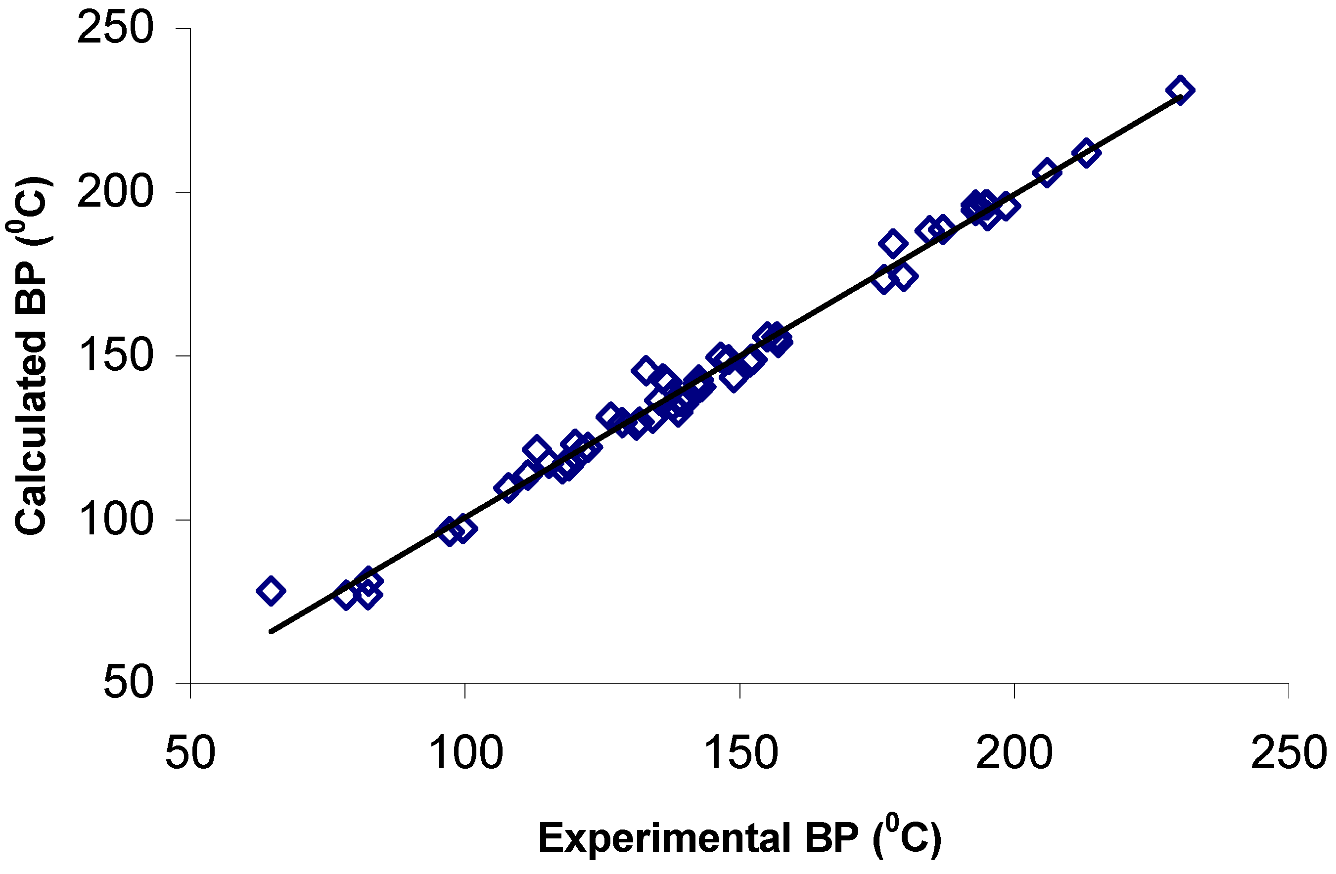
| 0.80 0.80 0.96 1.00 -0.90 | 53.964 χ – 49.003 s = 3.9°C r2 = 0.988 r = 0.994 | 0 |
| 0.80 0.80 0.96 1.00 -0.90 | 53.255 χ – 45.599 s = 2.6°C r2 = 0.994 r = 0.997 | 5 |
| Alcohol | Exp | Calc | Res | Calc* | Res* |
|---|---|---|---|---|---|
| methanol | 64.7 | 78.2 | -13.5 | * | * |
| ethanol | 78.3 | 77.0 | 1.3 | 78.8 | -0.5 |
| 1-propanol | 97.2 | 96.3 | 0.9 | 97.8 | -0.6 |
| 2-propanol | 82.3 | 77.2 | 5.1 | 78.9 | 3.4 |
| 1-butanol | 117.0 | 115.6 | 2.1 | 116.8 | 0.9 |
| 2-butanol | 99.6 | 97.2 | 2.4 | 98.7 | 0.9 |
| 2-M-1-propanol | 107.9 | 109.6 | -1.7 | 110.9 | -3.0 |
| 2-M-2-propanol | 82.4 | 81.3 | 1.1 | 83.0 | -0.6 |
| 1-pentanol | 137.8 | 134.9 | 3.0 | 135.8 | 2.0 |
| 2-pentanol | 119.0 | 116.5 | 2.5 | 117.7 | 1.3 |
| 3-pentanol | 115.3 | 117.2 | -1.9 | 118.5 | -3.2 |
| 2-M-1-butanol | 128.7 | 129.6 | -0.9 | 130.7 | -2.0 |
| 3-M-1-butanol | 131.2 | 128.9 | 2.3 | 129.9 | 1.3 |
| 2-M-2-butanol | 102.0 | 101.8 | 0.2 | 103.2 | -1.1 |
| 3-M-2-butanol | 111.5 | 113.6 | -2.1 | 114.9 | -3.4 |
| 2,2-MM-1-propanol | 113.1 | 121.4 | -8.3 | * | * |
| 1-hexanol | 157.0 | 154.1 | 2.9 | 154.8 | 2.2 |
| 2-hexanol | 139.9 | 135.8 | 4.2 | 136.7 | 3.2 |
| 3-hexanol | 135.4 | 136.5 | -1.1 | 137.5 | -2.1 |
| 2-M-1-pentanol | 148.0 | 148.9 | -0.9 | 149.7 | -1.7 |
| 3-M-1-pentanol | 152.4 | 148.9 | 3.5 | 149.7 | 2.7 |
| 4-M-1-pentanol | 151.8 | 148.2 | 3.6 | 149.0 | 2.8 |
| 2-M-2-pentanol | 121.4 | 121.0 | 0.4 | 122.2 | -0.8 |
| 3-M-2-pentanol | 134.2 | 131.1 | 3.2 | 132.1 | 2.1 |
| 4-M-2-pentanol | 131.7 | 129.8 | 1.9 | 130.9 | 0.9 |
| 2-M-3-pentanol | 126.6 | 131.4 | -4.8 | 132.4 | -5.8 |
| 3-M-2-pentanol | 122.4 | 122.2 | 0.2 | 123.4 | -1.0 |
| 2-ethyl-1-butanol | 146.5 | 149.7 | -3.2 | 150.5 | -4.0 |
| 2,2-MM-1-butanol | 136.8 | 141.8 | -5.0 | 142.7 | -5.9 |
| 2,3-MM-1-butanol | 149.0 | 143.5 | 5.6 | 144.3 | 4.7 |
| 3,3-MM-1-butanol | 143.0 | 140.6 | 2.4 | 141.6 | 1.5 |
| 2,3-MM-2-butanol | 118.6 | 117.3 | 1.3 | 118.6 | 0.0 |
| 3,3-MM-2-butanol | 120.0 | 123.1 | -3.1 | 124.2 | -4.2 |
| 1-heptanol | 176.3 | 173.4 | 2.9 | 173.9 | 2.4 |
| 3-heptanol | 156.8 | 155.8 | 1.0 | 156.5 | 0.3 |
| 4-heptanol | 155.0 | 155.8 | -0.8 | 156.5 | -1.5 |
| 2-M-2-hexanol | 142.5 | 140.3 | 2.2 | 141.2 | 1.3 |
| 3-M-3-hexanol | 142.4 | 141.5 | 0.9 | 142.4 | 0.0 |
| 3-E-3-hexanol | 142.5 | 142.7 | -0.2 | 143.6 | -1.1 |
| 2,3-MM-2-pentanol | 139.7 | 135.9 | 3.8 | 136.9 | 2.9 |
| 3,3-MM-2-pentanol | 133.0 | 143.5 | -10.5 | * | * |
| 2,2-MM-3-pentanol | 136.0 | 143.1 | -7.1 | * | * |
| 2,3-MM-3-pentanol | 139.0 | 136.3 | 2.7 | 137.3 | 1.7 |
| 2,4-MM-3-pentanol | 138.8 | 132.9 | 5.9 | 133.9 | 4.9 |
| 1-octanol | 195.2 | 192.7 | 2.5 | 192.9 | 2.3 |
| 2-octanol | 179.8 | 174.3 | 5.5 | 174.8 | 5.0 |
| 2-E-1-hexanol | 184.6 | 188.2 | -3.6 | 188.5 | -3.9 |
| 2,3,3-MMM-3-pentanol | 152.2 | 149.0 | 3.2 | 149.8 | 2.4 |
| 1-nonanol | 213.1 | 211.9 | 1.2 | 211.9 | 1.2 |
| 2-nonanol | 198.5 | 195.8 | 2.7 | 196.0 | 2.5 |
| 3-nonanol | 194.7 | 196.1 | -1.4 | 196.3 | -1.6 |
| 4-nonanol | 193.0 | 196.1 | -3.1 | 196.3 | -3.3 |
| 5-nonanol | 195.1 | 196.1 | -1.0 | 196.3 | -1.2 |
| 7-M-1-octanol | 206.0 | 206.0 | 0.0 | 206.0 | -0.0 |
| 2,6-MM-4-heptanol | 178.0 | 184.2 | -6.2 | * | * |
| 3,5-MM-4-heptanol | 187.0 | 188.7 | -1.7 | 189.0 | -2.0 |
| 3,5,5-MMM-1-hexanol | 193.0 | 194.4 | -1.4 | 194.6 | -1.6 |
| 1-decanol | 230.2 | 231.2 | -1.0 | 230.9 | -0.7 |

Concluding Remarks
Acknowledgments
References
- Todeschini, R.; Consonni, V. Handbook of Molecular Descriptors (Methods and Principles in Medicinal Chemistry. vol. 11, Mannhold, R., Kubinyi, H., Timmerman, H., Eds.; Wiley-VCH: New York, 2000. [Google Scholar]
- Devillers, J; Balaban, A. T. (Eds.) Topological Indices and Related Descriptors in QSAR and QSPR; Gordon and Breach: Amsterdam, 1999.
- Lučić, B.; Miličević, A.; Nikolić, S.; Trinajstić, N. On variable Wiener index. Ind. J. Chem. A 2003, 42, 1279–1282. [Google Scholar]
- Estrada, E. Three-dimensional generalized graph matrix, Harary descriptors and a generalized interatomic Lennard-Jones potential. J. Phys. Chem. A 2004, 108, 5468–5473. [Google Scholar]
- Estrada, E. Generalized Graph Matrix, Graph Geometry, Quantum Chemistry and the Optimal Description of Physicochemical Properties. J. Phys. Chem. A 2003, 107, 7482–7489. [Google Scholar]
- Estrada, E.; Gutierrez, Y. The Balaban J index in the multidimensional space of generalized topological indices. Generalizations and QSPR Match 2001, 44, 155–167. [Google Scholar]
- Estrada, E. Generalization of topological indices. Chem. Phys. Lett. 2001, 336, 248–252. [Google Scholar]
- Kier, L. B.; Hall, H. L. Molecular Connectivity. VII. Specific treatment of heteroatoms. J. Pharm. Sci. 1976, 65, 1806–1809. [Google Scholar]
- Kier, L. B.; Hall, L. H. Molecular Connectivity in Chemistry and Drug Research; Academic: New York, 1976. [Google Scholar]
- Randić, M. On characterization of molecular branching. J. Am. Chem. Soc. 1975, 97, 6609–6615. [Google Scholar]
- Kier, L. B.; Murray, W. J.; Randić, M.; Hall, L. H. Molecular connectivity V: Connectivity series concept applied to density. J. Pharm. Sci. 1976, 65, 1226–1230. [Google Scholar]
- Barysz, M.; Jashari, G.; Lall, R. S.; Srivastave, V. K.; Trinajstić, N. On the distance matrix of molecules containing heteroatoms. In Applications of Chemical Topology and Graph Theory; King., R. B., Ed.; Elsevier: Amsterdam, 1983; pp. 222–227. [Google Scholar]
- Balaban, A. T. Chemical graphs. 48. Topological index J for heteroatom-containing molecules taking into account periodicities of elements properties. Math. Chem. (MATCH) 1986, 21, 115–122. [Google Scholar]
- Ivanciuc, O; Ivanciuc, T.; Cabrol-Bass, D.; Balaban, T. Comparison of weighted schemes for molecular graph descriptors: Application in quantitative structure – retention relationship for alkylphenols in gas-liquid chromatography. J. Chem. Inf. Comput. Sci. 2000, 40, 732–743. [Google Scholar]
- Ivanciuc, O; Ivanciuc, T.; Balaban, T. Design of topological indices. Part 10. Parameters based on electronegativity and covalent radius for the computation of molecular graph descriptors for heteroatom-containing molecules. J. Chem. Inf. Comput. Sci. 1998, 38, 395–401. [Google Scholar]
- Balaban, A. T. Highly discriminating distance-based topological index. Chem. Phys. Lett. 1982, 80, 399–404. [Google Scholar]
- Antipin, I. S.; Arslanov, N. A.; Palyulin, V. A.; Konovalov, A. I.; Zefirov, N. S. Solvation topological index. Topological description of dispersion interaction (in Russian). Dokl. Akad. Nauk. SSSR 1991, 316, 925–927. [Google Scholar]
- Antipin, I. S.; Arslanov, N. A.; Palyulin, V. A.; Konovalov, A. I.; Zefirov, N. S. Prognosis of enthalpy[y of nonspecific salvation of organic nonelectrolytes (in Russian). Dokl. Akad. Nauk. SSSR 1993, 316, 173–176, [Chem. Abstr. 1993, 120, 133743]. [Google Scholar]
- Zefirov, N. S.; Palyulin, V. A. QSAR for boiling points of “small” sufides. Are the “High-Quality Structure-Property-Activity Regressions” the real high quality QSAR models?”. J. Chem. Inf. Comput. Sci. 2001, 41, 1022–1027. [Google Scholar]
- Katrizky, A. R.; Lobanov, V. S.; Karelson, M. CODESSA (COmprehensive Descriptors for Structural and Statistical Analysis). University of Florida: Gainesville. FL., 1995. [Google Scholar]
- Randić, M. Resolution of ambiguities in structure-property studies by use of orthogonal descriptors. J. Chem. Inf. Comput. Sci. 1991, 31, 311–320. [Google Scholar]
- Randić, M. Orthogonal molecular descriptors. New J. Chem. 1991, 15, 517–525. [Google Scholar]
- Randić, M. Correlation of enthalpy of octanes with orthogonal connectivity indices. J. Mol. Struct. (Theochem) 1991, 233, 45–59. [Google Scholar]
- Randić, M. Fitting of nonlinear regressions by orthogonalized power series. J. Comput. Chem. 1992, 14, 363–370. [Google Scholar]
- Wu, L.; Zhang, W-J. Comparison of different methods for variable selection. Anal. Chim. Acta 2001, 446, 477–483. [Google Scholar]
- Lučić, B.; Amić, D.; Trinajstić, N. Nonlinear multivariate regressions outperforms several concisely designed neural networks on three QSRP data set. J. Chem. Inf. Comput. Sci. 2000, 40, 403–413. [Google Scholar]
- Randić, M. Retro-regression – another important multivariate regression improvement. J. Chem. Inf. Comput. Sci. 2001, 41, 602–606. [Google Scholar]
- Randić, M.; Zupan, J. M. On the structural interpretation of topological indices. In "Topology in Chemistry. Discrete Mathematics of Molecules"; Rouvray, D. H., King, R. B., Eds.; Horwood Publishing Series in Chemical Science, Horwood Publ. Ltd.: Chichester, U.K., 2002; pp. 249–291. [Google Scholar]
- Randić, M.; Zupan, J. On intereptation of well-known topological indices. J. Chem. Inf. Comput. Sci. 2001, 41, 550–560. [Google Scholar]
- Randić, M.; Balaban, A. T.; Basak, S. C. On structural interpretation of several distance related topological indices. J. Chem. Inf. Comput. Sci. 2001, 41, 593–601. [Google Scholar]
- Randić, M.; Basak, N. Novel graphical matrix and novel distance based molecular descriptors. Croat. Chem. Acta. (in press).
- Randić, M. Novel graph theoretical approach to heteroatoms in quantitative structure-activity relationships. Chemometrics Intel. Lab. Systems 1991, 10, 213–227. [Google Scholar]
- Randić, M. On computation of optimal parameters for multivariate analysis of structure-property relationship. J. Comput. Chem. 1991, 12, 970–980. [Google Scholar]
- Randić, M.; Dobrowolski, J. Cz. Optimal molecular connectivity descriptors for nitrogen-containing molecules. Int. J. Quantum Chem. 1998, 70, 1209–1215. [Google Scholar]
- Randić, M. High quality structure-property regressions: boiling points of smaller alkanes. New J. Chem. 2000, 24, 165–171. [Google Scholar]
- Randić, M.; Basak, S. C. Construction of high quality structure-property-activity regressions: the boiling points of sulfides. J. Chem. Inf. Comput. Sci. 2000, 40, 899–905. [Google Scholar]
- Randić, M.; Pompe, M. The variable connectivity index 1χf versus the traditional descriptors: A comparative study of 1chif against descriptors of CODESSA. J. Chem. Inf. Comput. Sci. 2001, 41, 631–638. [Google Scholar]
- Randić, M.; Mills, D.; Basak, S. C. On use of variable connectivity index 1χf in QSAR: Toxicity of aliphatic ethers. J. Chem. Inf. Comput. Sci. 2001, 41, 614–618. [Google Scholar]
- Randić, M.; Pompe, M. The variable connectivity index 1χf versus the traditional molecular descriptors: A comparative study of 1χf against descriptors of CODESSA. J. Chem. Inf. Comput. Sci. 2001, 41, 631–638. [Google Scholar]
- Randić, M.; Plavšić, D.; Lerš, N. Variable connectivity index for cycle-containing structures. J. Chem. Inf. Comput. Sci. 2001, 41, 657–662. [Google Scholar]
- Randić, M.; Mills, D.; Basak, S. C. On use of variable connectivity index for characterization of amino acids. Int. J. Quantum Chem. Int. J. Quantum Chem. 2000, 80, 1199–1209. [Google Scholar]
- Liu, D.; Zhong, C. Modeling of the heat capacity of polymers with the variable connectivity index. Polymer J. 2002, 34, 954–961. [Google Scholar]
- Zhong, C.; He, J.; Xia, Z; Li, Y. Estimation of activity for Efavirenz analogous with the K 103N mutant of HIV reverse transcriptase using variable connectivity indices. Bioorg. Med. Chem. Lett. (submitted).
- Randić, M.; Pompe, M. On characterization of the CC double bond in alkenes. SAR & QSAR in Environ. Res. 1999, 10, 451–471. [Google Scholar]
- Randić, M.; Basak, S. C. Optimal molecular descriptors based on weighted path numbers. J. Chem. Inf. Comput. Sci. 1999, 39, 261–266. [Google Scholar]
- Randić, M.; Basak, S. C. A new descriptor for structure-property and structure-activity correlations. J. Chem. Inf. Comput. Sci. 2001, 41, 650–656. [Google Scholar]
- Randić, M.; Pompe, M. The variable molecular descriptors based on distance related matrices. J. Chem. Inf. Comput. Sci. 2001, 41, 575–581. [Google Scholar]
- Krenkel, G.; Castro, E. A.; Toropov, A. A. Improved molecular descriptors based on the optimization of correlation weights of local graph invariants. J. Mol. Struct. - Theochem. 2001, 542, 107–113. [Google Scholar]
- Randić, M.; Pompe, M. (to be published).
- Cammarata, A. Molecular topology and aqueous solubility of aliphatic alcohols. J. Pharm. Sci. 1979, 68, 839–842. [Google Scholar]
© 2004 by MDPI (http://www.mdpi.org). Reproduction is permitted for noncommercial purposes.
Share and Cite
Randić, M.; Pompe, M.; Mills, D.; Basak, S.C. Variable Connectivity Index as a Tool for Modeling Structure-Property Relationships. Molecules 2004, 9, 1177-1193. https://doi.org/10.3390/91201177
Randić M, Pompe M, Mills D, Basak SC. Variable Connectivity Index as a Tool for Modeling Structure-Property Relationships. Molecules. 2004; 9(12):1177-1193. https://doi.org/10.3390/91201177
Chicago/Turabian StyleRandić, Milan, Matevž Pompe, Denise Mills, and Subhash C. Basak. 2004. "Variable Connectivity Index as a Tool for Modeling Structure-Property Relationships" Molecules 9, no. 12: 1177-1193. https://doi.org/10.3390/91201177