Figure 1.
Repeatability of conductivity values on ageing of preparations PR1 and PR2. Average σ at the start (starting point conductivity) and 310th day with standard error (SE) intervals, measured at 25 °C and 1000 Hz when treatments are combined; PR1 (29 replicate solutions), PR2 (27 replicate solutions).
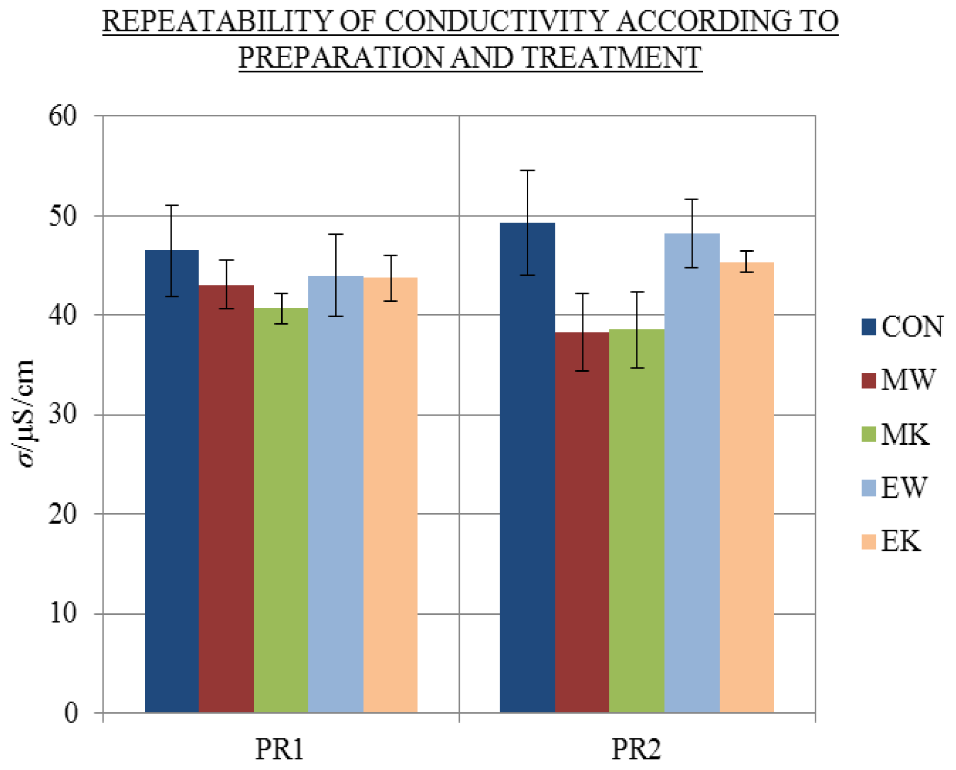
Figure 2.
Repeatability of average σ with standard error (SE) intervals at 25 °C and 1000 Hz after 310 days of ageing of 2 mL treatments CON (blue), MW (red), MK (green), EW (light blue) and EK (orange) of preparations PR1 and PR2; number of replicates, N (/), of PR1: CON (5), MW (7), MK (7), EW (5), EK (5); number of replicates of PR2: CON (5), MW (5), MK (7), EW (5), EK (5).
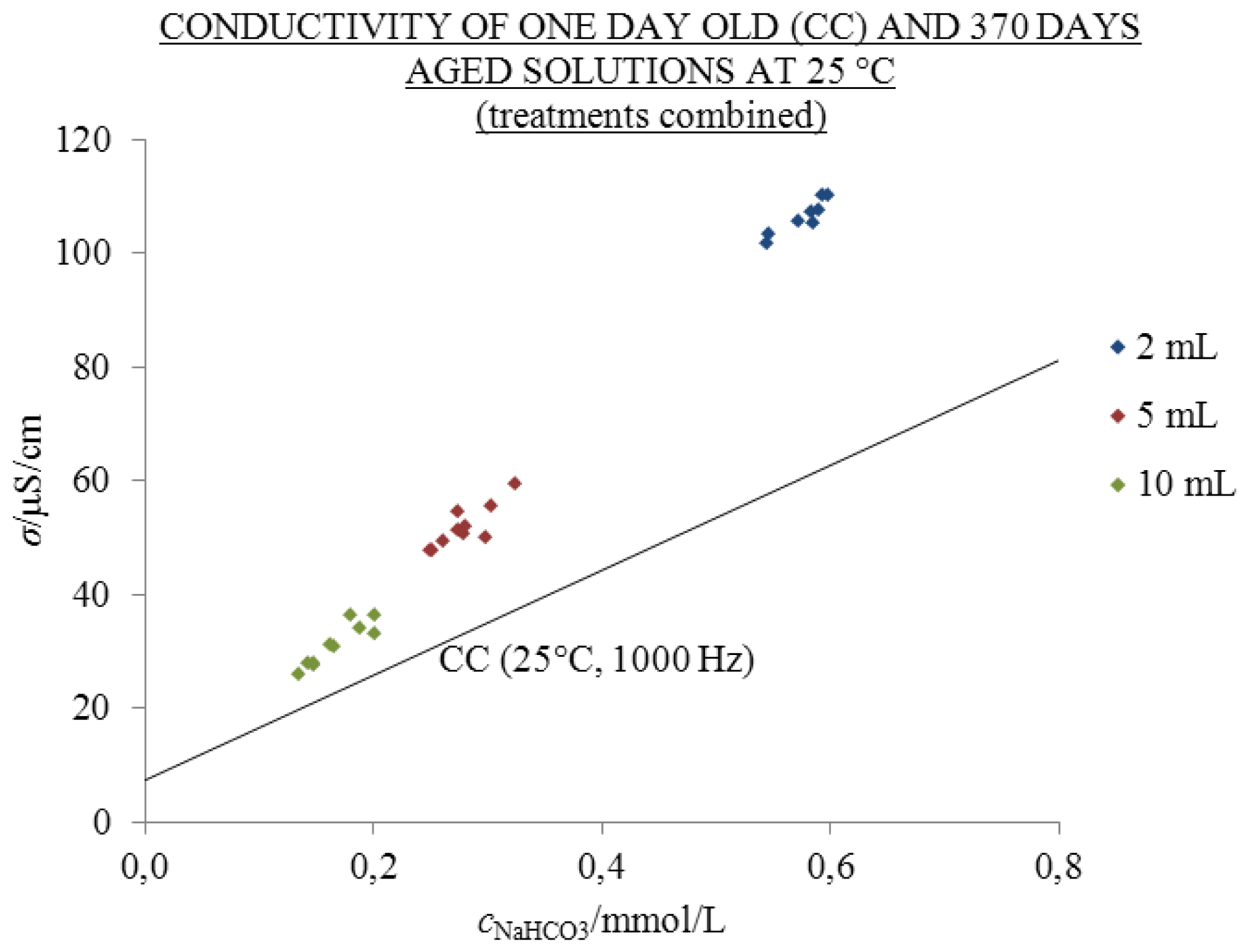
Figure 3.
σ at 25 °C and 1000 Hz as a function of cNaHCO3 of one-day-old (CC) and 370 days in 2 mL (blue), 5 mL (red) and 10 mL (green) volumes of 20 mL flasks under condition PR aged solutions; points in the graph represent individual measurements; number of replicate solutions, N (/): 2 mL (8), 5 mL (10), 10 mL (10). Treatments are combined; conductivity above the CC line is excess.
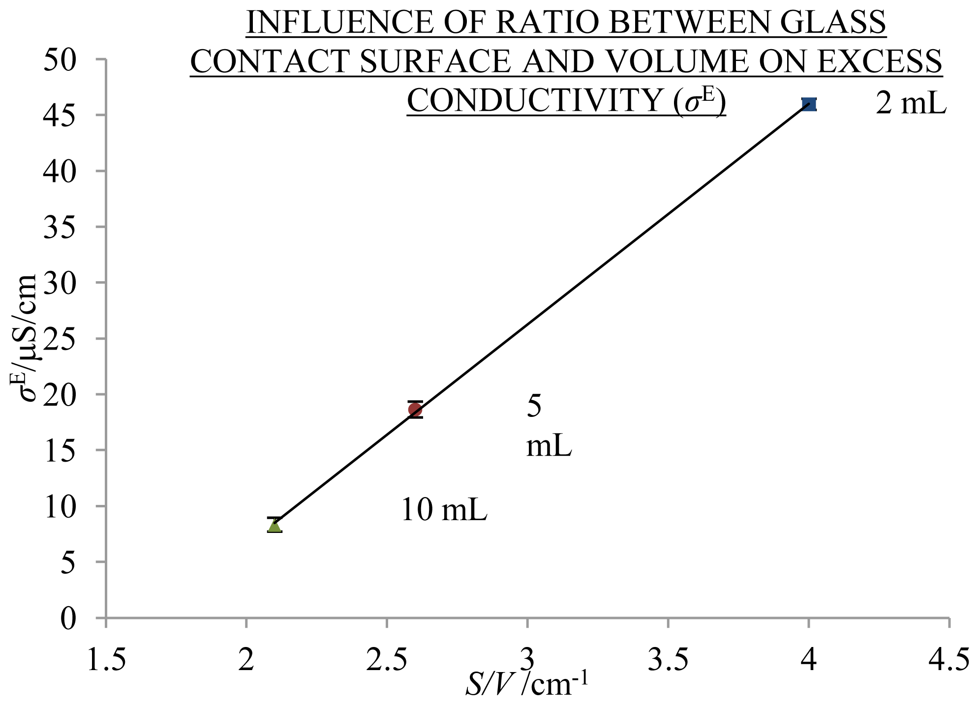
Figure 4.
Influence of the ratio of the glass contact surface and the volume, S/V, on average σE with SE intervals, measured at 25 °C and 1000 Hz, aged for 370 days in 2 mL (blue), 5 mL (red) and 10 mL (green) volumes of 20-mL flasks; number of replicate solutions, N (/): 2 mL (8), 5 mL (10), 10 mL (10). The abscissa starts at 1.5 cm−1.
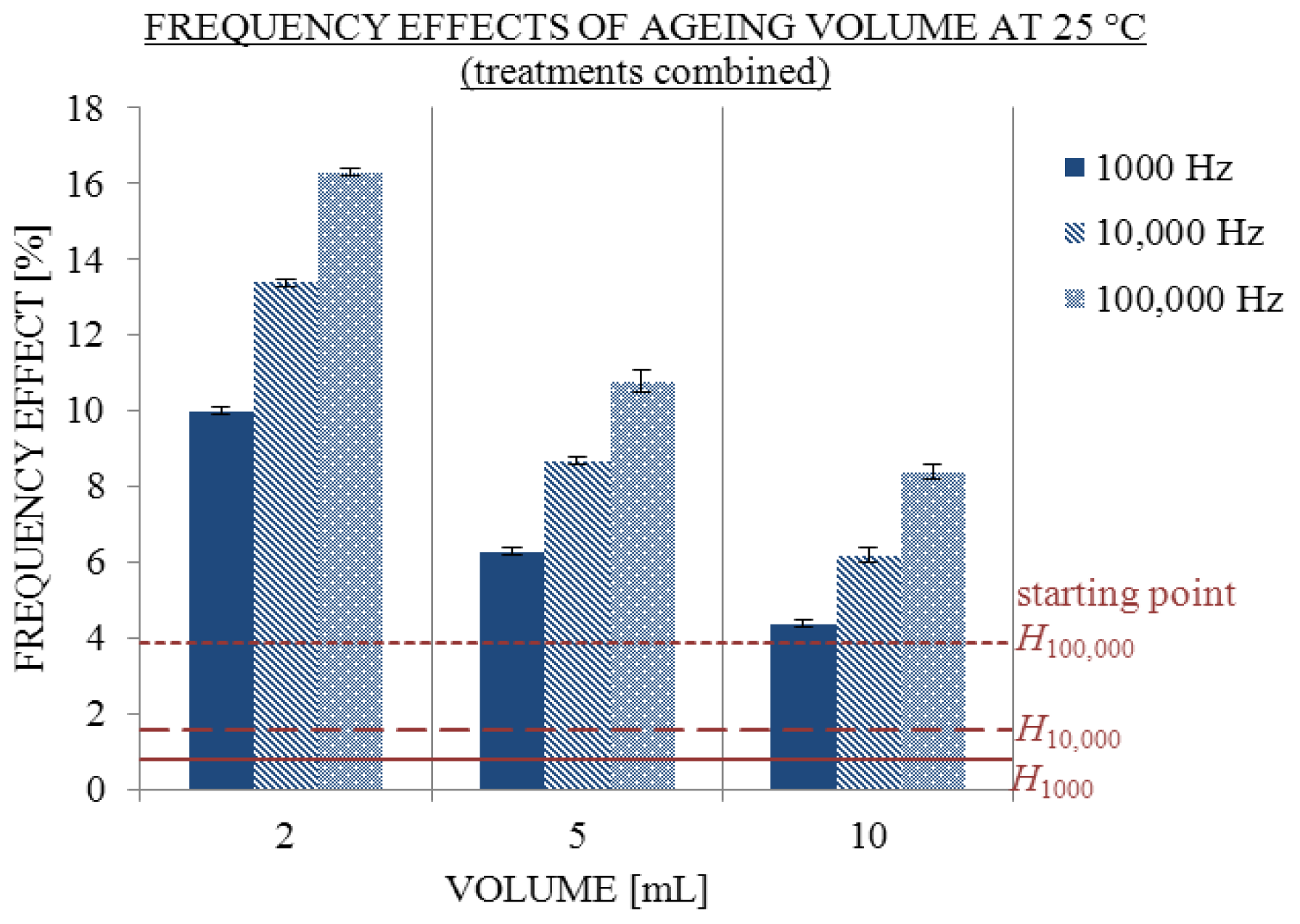
Figure 5.
Influence of ageing volume on average frequency effects with SE intervals at 1000 (filled), 10,000 (striped) and 100,000 Hz (dotted) 25 °C. Conductivity measured at start (starting point H) and 370th day in 2, 5 and 10 mL; number of replicate solutions, N (/): 2 mL (8), 5 mL (10), 10 mL (10).
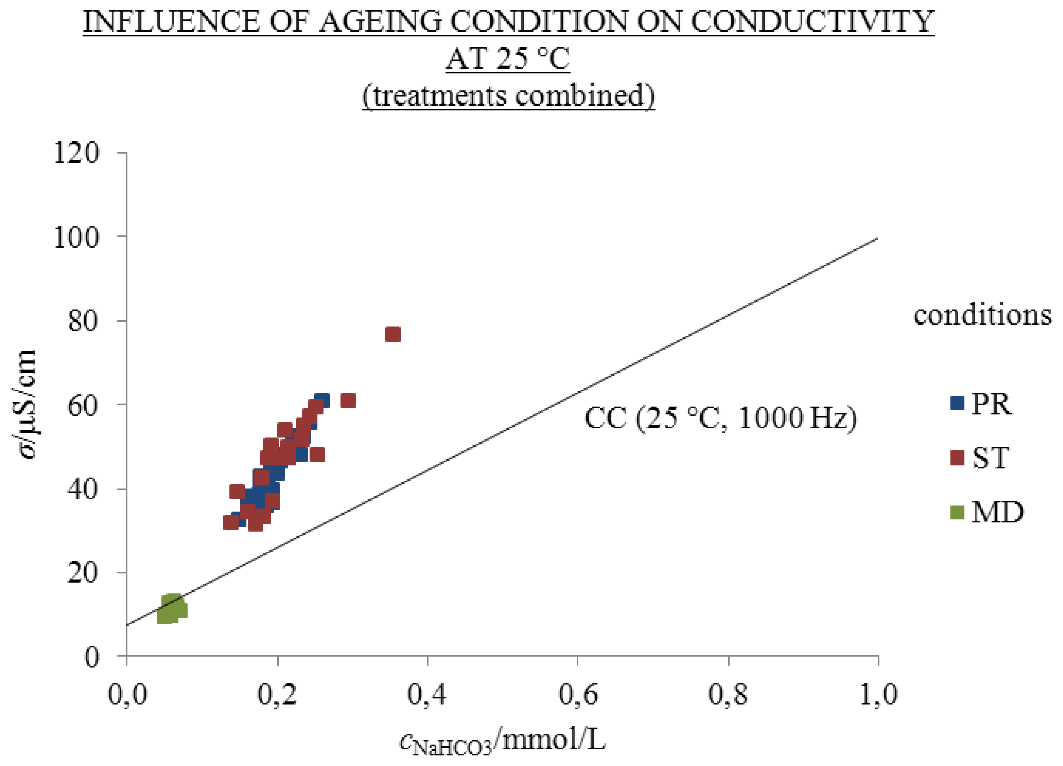
Figure 6.
σ at 25 °C and 1000 Hz as a function of cNaHCO3 of one day old (CC) and 310 days in 2 mL volume of 2.5 mL flasks under conditions PR (blue), ST (red) and MD (green) aged solutions; points in the graph represent individual measurements; number of replicate solutions, N (/): PR (28), ST (20), MD (20). Treatments are combined; conductivity above the CC line is excess.
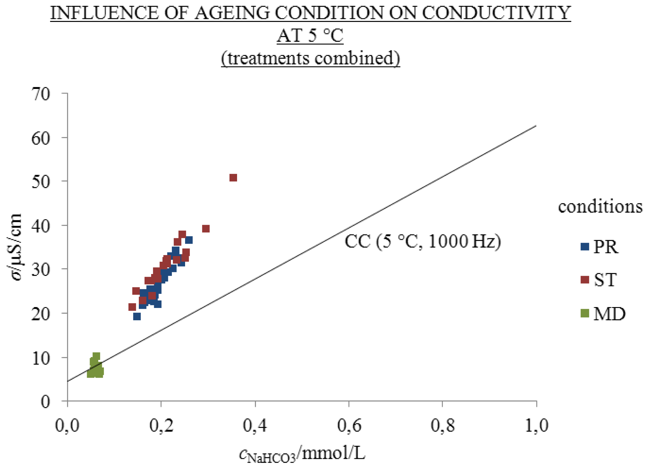
Figure 7.
σ at 5 °C and 1000 Hz as a function of cNaHCO3 of one day old (CC) and 310 days in 2 mL volume of 2.5 mL flasks under conditions PR (blue), ST (red) and MD (green) aged solutions; points in the graph represent individual measurements; number of replicate solutions, N (/): PR (28), ST (20), MD (20). Treatments are combined; conductivity above the CC line is excess.
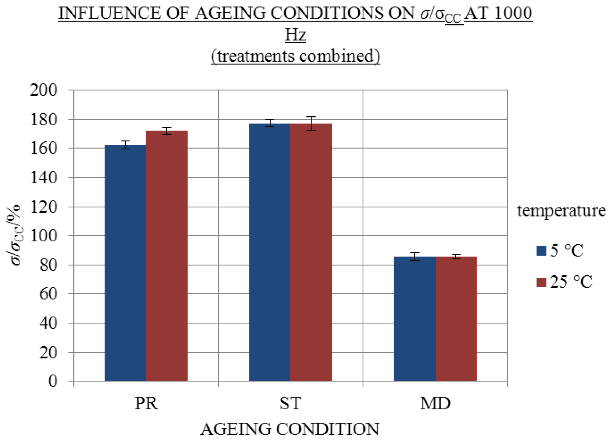
Figure 8.
Influence of ageing conditions PR, ST and MD on average σ/σCC with SE intervals measured at 1000 Hz 25 (red) and 5 °C (blue) (treatments combined); number of replicate solutions, N (/): PR (28), ST (20), MD (20). Solutions aged for 310 days.
Figure 8.
Influence of ageing conditions PR, ST and MD on average σ/σCC with SE intervals measured at 1000 Hz 25 (red) and 5 °C (blue) (treatments combined); number of replicate solutions, N (/): PR (28), ST (20), MD (20). Solutions aged for 310 days.
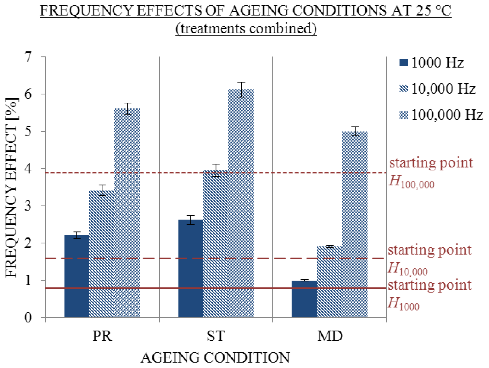
Figure 9.
Influence of ageing condition on frequency effects H; σ measured at 1000 (filled), 10,000 (striped) and 100,000 Hz (dotted) 25 °C with SE intervals, when the treatments are combined. Conductivity was measured initially (starting point H) and on 310th day under PR, ST and MD conditions; number of replicate solutions, N (/): PR (28), ST (20), MD (20).
Figure 10.
Average coefficients σ/σCC at 25 °C and 1000 Hz with SE intervals as a function of ratio of the volume of air above solution and the volume of solution (VCO2/VSOLUTION); treatments are combined. Solutions aged 310 or 370 days under the condition PR. Ordinate starts at 130%. N [/]: 0.01% of VCO2/VSOLUTION: 28; 0.04%: 10; 0.12%: 10; 0.35%: 8.
Figure 11.
Conductivity at 25 °C and 1000 Hz as a function of cNaHCO3 of one day old (CC) and aged solutions. Ageing for 310 days in 2 mL of 2.5 mL flasks under conditions PR, ST and MD (blue) and ageing for 370 days in 2, 5 and 10 mL of 20 mL flasks (red). Points in the graph represent individual measurements. Conductivity above CC is excess.
Figure 12.
Scheme of electrical treatment of solutions.
Figure 12.
Scheme of electrical treatment of solutions.
Figure 13.
Teflon holders for inserting the measuring cell into 2.5 and 20 mL flasks.
Figure 13.
Teflon holders for inserting the measuring cell into 2.5 and 20 mL flasks.
Figure 14.
Calibration curve of NaHCO3 solutions (in duplicate) at 25 °C and 1000 Hz; points in the graph represent individual measurements.
Figure 14.
Calibration curve of NaHCO3 solutions (in duplicate) at 25 °C and 1000 Hz; points in the graph represent individual measurements.
Table 1.
Average σ/σCC and relative standard errors (RSE) at 1000 Hz 25 and 5 °C of NaHCO3 solutions aged for 310 days in 2 mL volume of 2.5 mL flasks under conditions PR—exposed to daylight, ST—protected from daylight and MD—at −20 °C; treatments are combined.
Table 1.
Average σ/σCC and relative standard errors (RSE) at 1000 Hz 25 and 5 °C of NaHCO3 solutions aged for 310 days in 2 mL volume of 2.5 mL flasks under conditions PR—exposed to daylight, ST—protected from daylight and MD—at −20 °C; treatments are combined.
| Temperature (°C) | σ/σCC (%) ± RSE (%) |
|---|
|
|---|
| PR | ST | MD |
|---|
| 25 | 171.9% ± 1.4% | 176.8% ± 2.6% | 85.6% ± 1.8% |
| 5 | 162.3% ± 1.5% | 177.2% ± 1.5% | 85.6% ± 3.2% |
Table 2.
Influence of dissolved CO2 (VCO2/VSOLUTION) on σ/σCC of aged solutions. Conductivity measured at 25 °C and 1000 Hz, treatments are combined.
Table 2.
Influence of dissolved CO2 (VCO2/VSOLUTION) on σ/σCC of aged solutions. Conductivity measured at 25 °C and 1000 Hz, treatments are combined.
| Ageing | VFLASK | VSOLUTION | VAIR | VCO2/VSOLUTION | S/V | NaHCO3 | σ/σCC1000 |
|---|
|
|---|
| AVG | SE | AVG | SE | N |
|---|
|
|---|
| d | mL | mL | mL | % | cm−1 | mmol/L | mmol/L | % | % | / |
|---|
| 310 | 2.5 | 2 | 0.5 | 0.01 | 3.9 | 0.19 | 0.01 | 171.9 | 2.4 | 28 |
| 370 | 20 | 2 | 18 | 0.35 | 4.0 | 0.58 | 0.01 | 176.3 | 0.8 | 8 |
| 370 | 20 | 5 | 15 | 0.12 | 2.6 | 0.28 | 0.01 | 156.7 | 1.9 | 10 |
| 370 | 20 | 10 | 10 | 0.04 | 2.1 | 0.17 | 0.01 | 136.8 | 2.2 | 10 |
Table 3.
Used treatments.
Table 3.
Used treatments.
| Treatment | Donor | Abbreviation |
|---|
| no treatment—control | / | CON |
| mechanical treatment to 10C | Milli-q water | MW |
| KCl | MK |
| electrical treatment | Milli-q water | EW |
| KCl | EK |
Table 4.
Average conductivities of one-day-old NaHCO3 solutions (in duplicate) with deviations between the duplicates (Δ) measured at 25 and 5 °C and 1000 Hz.
Table 4.
Average conductivities of one-day-old NaHCO3 solutions (in duplicate) with deviations between the duplicates (Δ) measured at 25 and 5 °C and 1000 Hz.
| cNaHCO3 | σ (25 °C) | Δ (25 °C) | σ (5 °C) | Δ (5 °C) |
|---|
|
|---|
| mmol/L | μS/cm | μS/cm | μS/cm | μS/cm |
|---|
| 0.05 | 12.5 | 0.1 | 7.5 | 0.0 |
| 0.10 | 16.8 | 0.2 | 10.5 | 0.1 |
| 0.20 | 25.7 | 0.5 | 16.3 | 0.2 |
| 0.30 | 34.6 | 0.1 | 22.1 | 0.0 |
| 0.40 | 44.4 | 0.4 | 28.0 | 0.4 |
| 0.50 | 53.9 | 0.2 | 33.6 | 0.2 |
| 0.60 | 63.7 | 1.3 | 39.5 | 0.0 |
| 0.80 | 83.1 | 1.8 | 50.7 | 0.3 |
| 1.00 | 98.0 | 0.0 | / | / |
Table 5.
Equations of conductivity curves (CC) with deviations from linearity (R2); conductivity of one-day-old NaHCO3 solutions measured at 25 and 5 °C in 2.5 mL flasks. Conductivities, σCC, are in μS/cm, concentrations, cNaHCO3, in mmol/L.
Table 5.
Equations of conductivity curves (CC) with deviations from linearity (R2); conductivity of one-day-old NaHCO3 solutions measured at 25 and 5 °C in 2.5 mL flasks. Conductivities, σCC, are in μS/cm, concentrations, cNaHCO3, in mmol/L.
| T (°C) | 120 Hz | 1000 Hz | 10,000 Hz | 100,000 Hz |
|---|
| 25 | σCC = 90.1cNaHCO3 + 8 | σCC = 92.4cNaHCO3 + 7 | σCC = 93.4cNaHCO3 + 7 | σCC = 95.2cNaHCO3 + 8 |
| R2 = 0.9983 | R2 = 0.9983 | R2 = 0.9983 | R2 = 0.9983 |
| 5 | σCC = 56.7cNaHCO3 + 5 | σCC = 58.1cNaHCO3 + 5 | σCC = 59.0cNaHCO3 + 4 | σCC = 56.0cNaHCO3 + 2 |
| R2 = 0.9996 | R2 = 0.9997 | R2 = 0.9996 | R2 = 0.9973 |
Table 6.
Ageing conditions.
Table 6.
Ageing conditions.
| Condition | Influences |
|---|
| PR | exposed to daylight |
| ST | protected from daylight |
| MD | at low temperatures: −20 °C |


