Article

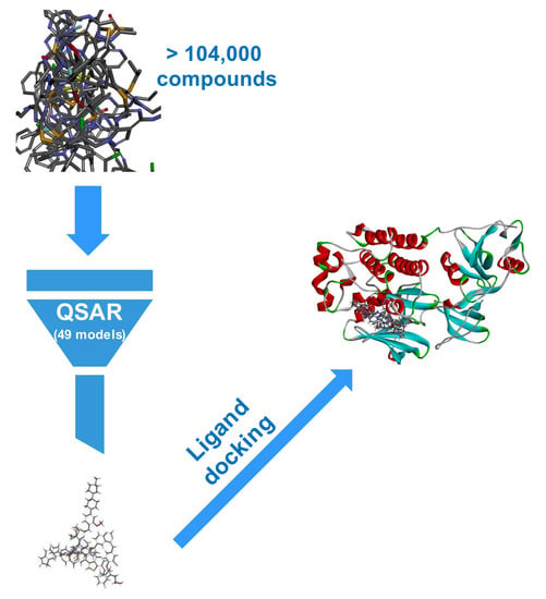
Use of QSAR Global Models and Molecular Docking for Developing New Inhibitors of c-src Tyrosine Kinase

1
Faculty of Pharmacy, Carol Davila University of Medicine and Pharmacy, 020956 Bucharest, Romania
2
Advanced Research and Development Center for Experimental Medicine (CEMEX), Grigore T. Popa, University of Medicine and Pharmacy of Iasi, 700115 Iasi, Romania
3
Department of Chemical Thermodynamics, Institute of Physical Chemistry “Ilie Murgulescu”, 060021 Bucharest, Romania
*
Author to whom correspondence should be addressed.
Int. J. Mol. Sci. 2020, 21(1), 19; https://doi.org/10.3390/ijms21010019
Submission received: 22 October 2019 / Revised: 15 December 2019 / Accepted: 16 December 2019 / Published: 18 December 2019
(This article belongs to the Special Issue QSAR and Chemoinformatics Tools for Modeling)

Abstract

:
A prototype of a family of at least nine members, cellular Src tyrosine kinase is a therapeutically interesting target because its inhibition might be of interest not only in a number of malignancies, but also in a diverse array of conditions, from neurodegenerative pathologies to certain viral infections. Computational methods in drug discovery are considerably cheaper than conventional methods and offer opportunities of screening very large numbers of compounds in conditions that would be simply impossible within the wet lab experimental settings. We explored the use of global quantitative structure-activity relationship (QSAR) models and molecular ligand docking in the discovery of new c-src tyrosine kinase inhibitors. Using a dataset of 1038 compounds from ChEMBL database, we developed over 350 QSAR classification models. A total of 49 models with reasonably good performance were selected and the models were assembled by stacking with a simple majority vote and used for the virtual screening of over 100,000 compounds. A total of 744 compounds were predicted by at least 50% of the QSAR models as active, 147 compounds were within the applicability domain and predicted by at least 75% of the models to be active. The latter 147 compounds were submitted to molecular ligand docking using AutoDock Vina and LeDock, and 89 were predicted to be active based on the energy of binding.

Graphical Abstract

1. Introduction

Src (c-src, pp60-src, or p60-src) is a nonreceptor, cytoplasmic tyrosine kinase, the first of its kind to be discovered (in the 1970s) in the living world, whereas the corresponding gene was the first oncogene to be uncovered [1]. It is the prototype of a larger family, comprising at least nine members, most of them with little activity in normal cells in the absence of stimulatory signals [2]. Src kinases have been suggested to be involved in the exacerbation of neurodegenerative pathologies, whereas their inhibition would diminish microgliosis and mitigate inflammation, findings that are in line with experimental effects seen for nonspecific src inhibitors such as bosutinib or LCB-03-0110 [3]. Nonclinical evidence has pointed to the inhibition of src kinases as a possible method of therapy for the pulmonary vascular remodeling and right ventricular hypertrophy in pulmonary hypertension [4], although several reports indicate that dual Abl/src inhibitor dasatinib may actually induce pulmonary hypertension [5,6,7]; it was more recently suggested that this dasatinib effect may in fact be independent of the src inhibition [7]. This family of kinases has been recently shown to be involved in the subgenomic RNA translation and replication of alpha-viruses, their inhibition being put forward as a potentially effective way of treating infections with such viral particles [8]. A constant interest for understanding the pharmacology of this class of compounds, as well as for developing new src inhibitors, may open the doors wide for multiple therapeutic applications for these inhibitors in a variety of pathologies.
The first member of this family (c-src) may play a more significant role than other members of the same family in certain pathologies or clinical contexts. For instance, c-src, but not Lyn and Fyn src kinases, is upregulated by hypoxia and has an important part in prostate cancer metastasis of hypoxic tumors (hypoxia is a negative prognostic factor in this malignancy) [9]. Furthermore, c-src tyrosin kinase has been shown to be abnormally activated or overexpressed in a number of different malignancies and to stimulate processes associated with tumor progression, such as proliferation, angiogenesis, or metastasis [10]. Src tyrosin kinase inhibitors have been explored as potential new therapeutic agents in a variety of malignancies such as melanoma (one such inhibitor demonstrating in vitro activity on a variety of melanoma cells, including some BRAFV600 mutant cells [11], but a report that src inhibition would induce melanogenesis in melanoma cells has also been published [12]), papillary thyroid carcinoma [13], clear-cell renal carcinoma [14], pancreatic [15], or ovarian cancer [16].
The space of the universe is expanding, but so is the “chemical space”. Currently PubChem includes some 96 million different chemical compounds [17], an impressive number, but minuscule when compared with the number of chemical compounds that might be synthesized in the coming years. GDB-17, probably the largest database of molecules up to date, included in 2015 no less than 166 billion compounds, and these are limited to only a few types of atoms (C, N, O, S, and halogens) and a maximum of 17 atoms per molecule [18]. Theoretical calculations using constraints for circumscribing the drug-like chemical space have suggested that the number of molecules obeying to the Lipinsky’s rules is about 1033 [19], an estimate intermediary between 1060 (as proposed earlier by R.S. Bohacek et al. [20]) and 1023 (as advanced later by P. Ertl. [21]). This raises questions regarding how to assess all these substances for their pharmacological, toxicological, or biological effects (in all contexts, for all targets etc.). While it is simply “mission: impossible” by the traditional route of wet lab experiments, the relatively cheap computing power available today may offer surprisingly good results (although far from perfect).
Built on three pillars (biological data, chemical knowledge, and modeling algorithms), QSAR (quantitative structure-activity relationship) [22] methodologies allow the development of computational tools for predicting with reasonable confidence (when validated appropriately) a wide variety of biological activities from the molecular structure of chemical compounds. Although the QSAR approaches have not gained in popularity as fast as the molecular docking modeling, the field has been far from being inert in the last decade or so, with various new approaches to the mathematical algorithms used or the biological activities explored [23]. The models developed and validated may then be applied for virtual screening of a large number of substances, allowing the quick identification of a sizeable number of compounds of interest (with certain activities or biological properties). Such virtual screening exercises may be further coupled with other computational methods, such as ligand-target docking for confirmation of activity [24,25]. Whereas the classical drug development process is very costly and tedious, computational methods have a high efficiency and are inexpensive [26]. In this context, we developed a set of QSAR models with different descriptors and machine learning classification algorithms, integrated by stacking, to be used for virtual screening of c-src tyrosin kinase inhibitors. A number of 49 QSAR models with reasonably good performance were selected and applied for the virtual screening of over 100,000 chemical compounds from the ZINC database [27]. A total of 147 compounds with the highest probability of being active were also assessed by molecular docking resulting in 89 compounds where the docking data were consistent with a hypothesis of activity. Data from ChEMBL and PubChem externally validated the virtual screening results for a number of compounds.

2. Results

2.1. Dataset Analysis

In our study, the final dataset included 1038 small organic molecules with a molecular weight varying from 188 to 1032 Da, a range usual in the QSAR modeling, with a median value of 390 Da and 75% of the values smaller than 440 Da. The number of atoms per molecule varied between 14 and 143, the median and mean values being 46 and 46.6, respectively. All molecules had at least one ring system and a maximum of six rings (with a median of three). Only 46 of the 1038 molecules satisfied the Lipinsky’s rule of five, of which 32 were labeled as “active” (ki < 1000 nM), and 14 as “inactive” (ki ≥ 1000 nM). The variability of the dataset by several simple constitutional descriptors or molecular properties is presented in Figure 1.
A dissimilarity matrix based on the Gower distance was computed (the Gower distance is appropriate for data of a heterogeneous nature), using 783 most relevant descriptors (that remained after removing autocorrelated and quasi-constant features). Although Gower distance takes values between 0 and 1, because it tends to give larger weights to binary variables [28], we rescaled the distance matrix and plotted it as a dissimilarity plot (Figure 2). Before rescaling the maximum value of the Gower distance was 0.404, following rescaling it became 1. The median (scaled) dissimilarity values were mostly around 0.2–0.3, suggesting that the chemical diversity in the dataset was rather limited (Supplementary Figures S1–S3).

2.2. Performances of Models in Nested Cross-Validation

Using a variety of classification algorithms (random forests, support vector machines, adaboost M1, Bayesian Additive Regression Trees, C5.0, and binomial regression), of feature selection methods (17), and numbers of features (between 3 and 40—for instance, for binomial regression we used models with 3, 5, 10, and 20 features, and thus the number of models built for this classifier was 68), a total number of over 350 models were built and their performance was assessed by nested cross-validation. Only models with an acceptable performance (defined as having both a balanced accuracy higher than 70% and a positive predictive value higher than 70% in the nested cross-validation) were selected (Table 1). In instances when several models (with different numbers of features) had good performance for the same classifier and selection algorithm (over the threshold of 70%), we only tabulated the model we judged as best (highest average between balanced accuracy and positive predictive value (PPV), and for equal value of the average giving preference to higher PPV). Numbers of true positives, true negatives, false positives, and false negatives, allowing computation of other performance metrics are available in Supplementary Table S2.
As the dataset includes 1038 compounds, of which 286 are active and 752 inactive, the most probable random accuracy (Q2, rnd) [29,30] may be estimated to 60.08% (286 × 286 + 752 × 752)/(1038 × 1038). As shown by the last column in Table 1, our models have a superiority of about 20–24% over random accuracy. However, the concept of random accuracy assumes that the correct classification of the two classes is of equal importance; in fact, in our case, we were more interested in correctly predicting the active compounds (i.e., optimizing the PPV was more important than Q2). The models were thus not optimized to increase the global accuracy, but rather both balanced accuracy and PPV.
As the models applied in the nested cross-validation are always based on only a subset of the data, the estimation of performance should be conservative (i.e., applying the selected models on the whole dataset has better performance).

2.3. Y-Randomization Test

As expected, despite following the same steps in building the models, scrambling the activity labels had a strong impact on the performance of the models, which was clearly inferior to those based on the initial (unscrambled) data: the average balanced accuracy of all 10 y-scrambling tests (nested cross-validation performed in the same conditions and following the same pre-processing as the true data) was 50.23%, with a standard deviation of 0.59% (minimum value 49.73% and maximum 51.45%). In a similar way, the mean value of the positive predictive (PPV) was 20.38%, and its value varied between 0.00% and 30.00%. This provides reassurance that the performance of the models is not the result of mere chance, but rather reflects a true relationship between the descriptors and the inhibitory activity on c-src tyrosine kinase.

2.4. Descriptors Associated with c-src Inhibitory Activity

While for all models the number of features was relatively high (in most cases between 20 and 30), the largest predictive effect could be attributed to no more than five features. For instance, in the case of random forest, using ANOVA as a feature selection (filtering) algorithm, with 23 features, the area under the receiver operating characteristic (ROC) curve (AUC) was 82.56% and the balanced accuracy 70.24%; however, using only the first most important five molecular descriptors, the AUC was 77.53%, and the balanced accuracy 66.39%. Although there was an improvement for the higher number of features (23), the first five explained the largest part of the variability in the training and testing datasets. We therefore focused on the first five descriptors selected by each of the 17 selection algorithms and found that most algorithms identified the same features as being the most important. These are shown in Table 2 (and descriptor values in Supplementary Table S3).

2.5. Virtual Screening and External Validation

We applied the models to the 104,619 ZINC compounds and ranked them based on the percentage of models predicting the compounds as active. Using a threshold of 50% (i.e., compounds predicted to be “active“ by more than 50% of all models applied) 744 compounds were identified. Our validation data (using the predictions on the test sets from the nested cross-validation) indicated that the PPV for this threshold was 78.57%. Increasing the decision threshold to 75% the number of compounds decreased to 158, but after eliminating the compounds that had been part of the training set and the duplicates (multiple ZINC ids may correspond to the same substance), their number decreased to 115 (Table S2); the validation data indicated a PPV value for this threshold of 85.43%. For a threshold of 90% the PPV in the validation was also close to 90% (90.1%), but the number of unique compounds was limited to 37.
For external validation purposes, we searched PubChem and ChEMBL for biological data related to the activity of the predicted compounds on the src tyrosine kinase, so as to have at least partial confirmation on the accuracy of the predictions. We found that among the 115 substances predicted as being active, for nine compounds (i.e., 7.83%) there is available evidence that they are active on the c-src tyrosine kinase. We could not find ki values for the nine compounds, but in most cases rather mean inhibition (as a percentage) at 1.0 or 0.1 μM was available. Taking into account that IC50 values are always higher than ki values for a competitive inhibitor, and the fact that percent inhibition is dependent on both substrate and inhibitor concentration, we considered as active compounds those with inhibition values of at least 30%. When a compound was labeled as “active” on the src target in one of the two public databases without further information on the endpoint or bioassay used, we also considered that compound as active (that was the case for balamapimod, reported by PubChem). Of the nine compounds labeled by us as “active”, three had a mean inhibition higher than 50%, one had a ki less than 1000 nM (20 nM to be precise), one was stated as “active” by PubChem with no further information and four had a mean% inhibition between 30% and 42.23% at 1 μM). A total of 34 additional substances (29.56%), predicted by the large majority of models as being active, were in fact proven to be inactive on src-tyrosine kinase, whereas 72 of the substances (62.61%) predicted to be active, seem to have never been tested for their effect on src tyrosine kinase. If the 43 compounds that were indeed tested were representative for the rest, the rate of success for the predictions would be 20.93%.

2.6. Applicability Domain

The “applicability domain” (AD) is a concept meant to evaluate if a model may be validly applied to predict the effect of a candidate compound; such validity is conditioned on the satisfaction of the assumptions applied in the construction of the model [31]. If the new substance whose activity we are trying to predict differs substantially from those on which a QSAR a model was based, such a prediction cannot be trusted. Therefore, assessing the AD for model is of paramount importance if that model is to be used for predictions, and a wide range of methods have been proposed in the literature for this purpose, each with its own advantages and flaws [32].
We used a variety of algorithms to assess the applicability domain for the predictions of the QSAR virtual screening by different models. Using the method by Roy et al. (2015) [33], which considers as an outlier each compound with a value outside the mean ± standard deviation, none of the compounds predicted by more than 50% of our models to be active were outside of the applicability model. This was not very surprising, because that method uses a decision tree based on three standard deviations, whereas we capped, centered, and scaled values to two standard deviations. Using the Kernel Density Estimation Outlier Score (KDEOS) algorithm (with a minimum of three and a maximum of 10 neighbors), which is based on a number of k-nearest neighbors, the number of outliers among the 744 compounds predicted as active by the majority of the QSAR models was small for each model, and not higher than 15% of the total number (with a median proportion toward 5%). Selecting the compounds after filtering them based on the applicability model did not change the hierarchization of the compounds predicted as active. The Influenced Outlierness (INFLO) algorithm (with k = 5), which is also based on a number of k-nearest neighbors, but taking into account a “a reverse nearest neighborhood set”, and that of F. Sahigara et al. (2013), which not only uses k-nearest neighbors, but also individual decision threshold for each data point of the training sample [34], identified a much larger proportion of compounds as outside the applicability method: for the latter, for instance, the proportion of outliers varied (for the different models) between 1.75% and 44.35%, with a median of 32.39% of the total of 744 compounds (Figure 3). A number of 147 compounds (of which five had been in the training dataset) were predicted by 75% of the models as being active, after limiting the votes to those compounds that were within the applicability domain estimated with the F. Sahigara et al. (2013) method [34]. All compounds identified by the virtual screening (before checking the applicability domain) fell for at least some of the models within the applicability domain, but the degree of confidence in the predictions changed after checking for the applicability domain.

2.7. Molecular Docking

In order to assess the performance of docking for the two software programs used (AutoDock Vina [35] and LeDock [36]) we first compared the estimated energies of binding for 175 compounds of the training set, with known activities on the target enzyme. With LeDock, the mean binding energy in the active compound group was −8.02 kcal/mol, whereas in the inactive compound group it was −7.29 kcal/mol (p < 10−7, Welch t-test). For the very active compounds (ki < 20 nM), the mean binding energy was −8.43 kcal/mol (p < 10−8 versus all inactive compounds, Welch t-test). Using the “cutpointr” package, an optimal cut-off was found at an energy of binding of −7.17 kcal/mol, which ensured an accuracy of 70.29%, with high sensitivity (90%), but low specificity (44%). In order to minimize the false positive, a cut-off point of −9.21 kcal/mol was necessary; at this level the specificity was 100% (i.e., none of the inactive compounds had such a low energy of binding in the docking runs), but with a very low sensitivity (only 9% of the active compounds had this low estimated energy of binding) (Figure 4). As our interest was to minimize the false-positive rate, we docked the 147 compounds predicted by the QSAR models to be active and within the applicability domain and somewhat surprisingly no less than 89 of them (61.22%) had such a low energy of binding, in other words they could be considered as active (Table 3). Considering that in our training subset, the sensitivity at this cut-off point (−9.21 kcal/mol) was only 9%, this high value does suggest that an important proportion of the compounds predicted by the QSAR models to be active might be indeed active, although when using docking one must be very cautious [37]. The root-mean-square deviation (RMSD) computed for the first cluster of poses of the ANP was 1.25, under the conventional threshold of 2.0, which may be considered reasonably well. The visual examination of the pose indicated that the ring pose was very well predicted, whereas the side chain prediction was less accurate (Figure 5). Of the 89 compounds of Table 3, 34 (38.20%) have already been reported to inhibit one or multiple tyrosine kinases.
Following the suggestion of one of the reviewers of this paper, we also submitted the 89 compounds to the online version of PASS [38], a software that predicts potential activities for chemical compounds. A total of 24 out of the 89 compounds (26.97%) were predicted to be active on the src tyrosine kinase and 62 of the 89 compounds were predicted to be active on at least one or multiple kinases (Table S4, Supplementary Information). Nevertheless, PASS predictions are also affected by limitations, because Pf-562271, a compound that was in our training set, was not detected at all as a src-tyrosine kinase inhibitor. Gw683134a, which based on the ChEMBL data causes a 36.99% inhibition of c-src tyrosine kinase at 1 μM, was not predicted as an inhibitor at all. Bx-795, which also at 1 μM causes a 27–30% inhibition of human c-src and 77–90% inhibition of Gallus gallus c-src, was also not predicted as an inhibitor. As for lapatinib, the probabilities to be active and to be inactive predicted by PASS were only 0.086 and 0.053, respectively.
AutoDock Vina performance was inferior to that of LeDock: on the same 175 compounds from the training set, the mean energy of binding was −10.30 kcal/mol for the active compounds and −10.03 kcal/mol for the inactive (p = 0.21, Welch t-test). An optimal cut-off for the AutoDock Vina compounds was at −9.26 kcal/mol, which ensured an accuracy of only 62.86%, with a sensitivity of 87.00% and a specificity of only 30.67%. As the performance of Vina was inferior to that of LeDock, we preferred to use only LeDock for virtual screening.
Computing various ligand efficiency metrics did not improve the predictions in the case of LeDock results: the accuracy rather decreased with all ligand efficiency measures attempted. In the case of AutoDock Vina, using different ligand efficiency measures changed the values of accuracy, sensitivity, and specificity, with no spectacular improvement. For instance, dividing the energy of binding to the molecular weight decreased sensitivity (from 87% to 43%), increased specificity (from 30.67% to 81.33%), and slightly increased the AUC (from 56.85% to 62.87%), but it also slightly decreased the accuracy (from 62.86% to 59.43%). Of the different ligand efficiency measures, for the AutoDock Vina results the best was obtained by dividing the energy of binding to the squared Ghose–Crippen octanol-water partition coefficient: 78% sensitivity, 49.33% specificity, 65.71% accuracy, and 65.05% AUC. Even with this ligand efficiency measure, the results were inferior to those obtained with LeDock based on the energies of binding.

3. Discussion

Several studies of QSAR models for c-src tyrosine kinase inhibitors have been published up to date in the scientific literature. Five such studies have explored the use of 3D-QSAR, and all of them used a relatively small number of compounds (80, 42, 156, and 39, respectively), with the same basic chemical structure within each study (pyrrolo-pyrimidine, quinazoline, anilinoquinazoline and quinolinecarbonitrile, quinolinecarbonitrile, and 4,6-substituted-(diaphenylamino)quinazolines); they could, therefore, be considered “local” models [39,40,41,42]. In the QSAR field, the term “local” is used to designate models based on a data set consisting of compounds related by their chemical structure, unlike global models, that are based on data sets consisting of structurally diverse chemical substances [43]. Another paper reported on the use of 2D-QSAR for c-src inhibitors, but these models were also local, focused on ethynyl-3-quinolinecarbonitriles [44]. Therefore, our study is the first one focused on global QSAR models for inhibitors targeting the c-src tyrosine kinase. It has been argued (and it stands to reason) that local models tend to have limited predictive power, even when their apparent performance indicates that they are robust [43]. Our global models are expected to have a higher predictive power, as partially confirmed in our external validation.
By far the most important descriptor in our work, identified by multiple feature selection algorithms, was SpMax4_Bh(m), the largest eigenvalue n. 4 of Burden matrix weighted by mass. This has not generally been reported in previous works as correlating with pharmacological activities. Other two Burden eigenvalues (SpMax3_Bh(m), SpMax5_Bh(m)) have also been among the most important descriptors correlating with the inhibition of c-src. SpMax3_Bh(m) has been used in predicting depuration rate constants for environmental pollutants of the polychlorinated biphenyls group [45], and the less relevant (in our case) SpMax6_Bh(m) has been used to predict chronic toxicity of substances to Pseudokirchneriella subcapitata [46]. The second most important descriptor for our data set was DECC (eccentric topologic index), which has been previously reported to be important in the prediction of monoamine oxidase A (MAO-A) activity [47,48], placental barrier permeability [49], and gas chromatographic retention times [50]. F06[C-N] was used in a model to describe the anti-proliferative effect of phenyl 4-(2-oxoimidazolidin-1-yl)-benzenesulfonates (local QSAR model) [51], antimalaric effect [52], or skin permeability of substances [53]. P_VSA_MR_6 has also been used for modeling of skin permeability [53], whereas we identified the use of Chi1_EA(dm) only for the QSPR modeling of fluorescence properties of a number of fluorescent dyes [54]. The aromatic nitrogen (N-073) has been shown to correlate positively with HIV-1 integrase activity inhibition [55] and negatively with the inhibition of the fibroblast growth factor (FGFR) [56]. We found no previous reports on the use of the Balaban distance connectivity index (J_D) in other models in the biological field, neither of the F05[C-N].
Rarely, the 49 QSAR models with similarly good performance converged in their predictions. Only eight compounds were predicted by all models to be active, and half of them (n = 4) were already in the training data set; for the large majority of compounds at least one or more of the models had contradictory results. This illustrates the need to avoid making decisions based on the results of a single or a small number of models.
As shown in the results section, for nine compounds (7.83% of the 115 substances with the best predictions) it has been confirmed that they are active. How good is such a measure for a virtual screening exercise? If we compare it with the PPV value in the nested cross-validation, the results are rather disappointing and indicate that one should always be cautious in interpreting results even when using double cross-validation, because the real world data are likely to be different from the data set used for training and testing. For instance, it is likely that the proportion of actives in the available data set used for the construction of the models is higher than the proportion of actives in the “real world“ (i.e., the wide chemical space used for virtual screening), and this may lead to a decrease in the positive predictive value in the real world. However, if we compare the results of the virtual screening with those of the most costly high throughput screening (HTS), the results are noteworthy. It has been reported that the hit rate of HTS should be expected to be less than 1% [57] and even less than 0.1% or 0.01% [58]. In one study, adding a computer-aided virtual screen was able to increase the screening hit proportion to 5.8% [57]. Thus, our success rate of at least 7.83% is reasonably good. If we compute the confirmation rate against the compounds that were assessed for their effect on src-tyrosine kinase (20.93%), the results are even better. As another positive aspect, more than a quarter of our predictions were supported by the PASS online software. Our virtual screening results showed, however, additional interesting facts.
A total of 16 additional false positives were in fact reported to be active on other members of the src family members, particularly Yes1 tyrosine kinase. This suggests that although our virtual screening exercise failed in multiple cases, the failure was often not far from the true target. Thus, from a total of 43 molecules that were tested for their effects on the src and other tyrosine kinases, 58.14% (25 compounds) were inhibitors of one or several members of the src-tyrosine kinase family (most often Yes1, sometimes also LCK or LYN tyrosin kinase).
Other false positives of the virtual screening exercise are inhibitors of proteins that src tyrosine kinase interacts directly, either activating them or being activated by them. It is known, for instance, that EGFR (epidermal growth factor receptor) can be activated by src without the presence of the EGFR ligand and that there is a direct correlation between EGFR overexpression and src activation [59]. Rather surprisingly for us, 13 compounds wrongly predicted by our models to be src tyrosine kinase inhibitors, are in fact inhibitors of EGFR, and 10 additional compounds that were inactive on src or other members of src family, were reported to be inhibitors of EGFR. Most of these 10 additional compounds (as well as most of the compounds active on src or Yes1 tyrosine kinase) are also active on ErbB4, and it has been reported that ErbB4-derived phosphopeptides are able to interact with the SH2 domain of src [60], that following stimulation by EGF, c-src is rapidly recruited to ErbB receptor complexes [61] and that activated src binds to ERBB4s80 (E4ICD), a cleaved fragment of ERBB4 [62]. Moreover, dasatinib, described often as a src inhibitor [63], has also shown to be one of the most potent ligands of ErbB4 [64]. Defactinib, apparently a false positive of our virtual screening is a potent FAK (focal adhesion kinase) inhibitor; it is known that FAK and nonreceptor src tyrosin kinase are both part of a focal adhesion complex (together with other structural, enzymatic, or adapter proteins), where they interact directly [65]. Three false positives of the virtual screening results were KIT and PDGFR inhibitors; KIT promotes phosphorylation of src and is activated by src [66], while src and PDGFR interact and phosphorylate each other at certain Tyr positions [67].
Such findings (compounds inactive on c-src tyrosine kinase, but active on kinases from the same kinase family or signaling pathway) tend to suggest that where the QSAR virtual screening fails is often not far from the target (but this is nonetheless a failure). How could these failures be explained, considering that multiple models converge in predicting a certain molecule as active on the target of interest (src tyrosine kinase)? It seems that the models manage to predict the tyrosine kinase properties of certain compounds, without having sufficient specificity to always separate those active on src from those active on other tyrosine kinases. We hypothesize that the training set is too small and does not include (a sufficient number of) molecules with selective src inhibitory properties; we intend to evaluate whether extending the data set with additional molecules inactive on src but active on other tyrosine kinases may improve the results of the virtual screening. It is also worth exploring the combining of more diverse descriptor sets in the final assembly of models with a view of improving the performance of the virtual screening.
Among the results produced by our virtual screening there is a sizeable number of antiviral molecules (vedroprevir, daclatasvir, ciluprevir, deleobuvir, ledipasvir, faldaprevir, tegobuvir, elbasvir, ombitasvir, narlaprevir), all of them approved or developed against hepatitis C viruses. They either target the NS3/NS4A (vedroprevir, ciluprevir, faldaprevir, narlaprevir) [68] or NS5A (daclatasvir, elbasvir, ombitasvir, ledipasvir) [69] or NS5B (deleobuvir, tegobuvir) [70] nonstructural proteins of the virus. It is not very surprising to see inhibitors of NS5A and NS5B here, considering that is already known that NS5A protein binds to tyrosine kinases from the src-family [71], and c-src is an essential host protein involved in the formation of the HCV replication complex, together with NS5A and NS5B [72]. It was less expected to see also inhibitors of the NS3/NS4A among the results of the virtual screening, because no direct interaction was reported between the Ns3/NS4A complex and src tyrosine kinase. This list of HCV antivirals might consist only of false positives, but it is worth testing in wet lab experiments.
The docking applied to 147 compounds predicted with a high probability by the QSAR models to be active, reduced their number to about 61% of the initial size. For a number (27.78%) of these 89 compounds, predicted by both QSAR and docking to be active, data available in ChEMBL or PubChem (from a single wet lab test) indicate that they are inactive, and for others (6.67%), that they are active, as discussed for the QSAR models. This suggests that computational results have to be interpreted with caution even when different models, with different methodologies and assumptions, converge in their predictions. On the other hand, the last decade has witnessed a growing realization of what has been dubbed “the reproducibility crisis”, ascribed to the inappropriate quality of antibodies used as reagents [73], insufficiently described methodologies or simply to the biology itself [74]. Whereas positive findings have often not been reproduced when experiments were repeated in other laboratories, it is not impossible that negative findings could also not be replicable and some of the compounds shown by databases to be inactive might, as a matter of fact, be active. However, in the absence of contrary evidence, such compounds have to be considered inactive.
Virtual screening results are also influenced by potential errors affecting the input data: if the wet lab data that were used to generate the models are affected by errors, they will propagate forward in the models built and in the predictions made on new compounds. The estimated docking energies are also potentially affected by errors (in our estimation the accuracy was about 70%, but the large number of compounds used in screening may differ more from our data set, and thus accuracy might be lower). Moreover, docking methods are also prone to errors, there are often discrepancies between docking results and ligand-based studies, and there are multiple cases where top compounds identified by docking methods failed in wet lab experiments [37].

4. Materials and Methods

4.1. Dataset

The dataset (Table S1) was downloaded from ChEMBL (https://www.ebi.ac.uk/chembl) and included experimental data for c-src as a target (target code CHEMBL267). Only the records with ki values expressed in nM were kept. Records with “=” values in the field “Relation” were kept for analysis and labeled as “active” if ki < 1000 nM and “inactive” if ki ≥ 1000 nM; records with “>” or “<” values in the field “Relation” were kept for analysis only if they allowed unequivocal classification (e.g., records with ki > 5000 nM were kept and labeled as “inactive”, whereas those with ki > 100 nM were discarded; similarly, records with ki < 5000 nM were discarded). A threshold of 1000 nM for the formal discrimination between “active” and “inactive” compounds is usual in the field and has been used in other publications [75]. We used classification rather than regression, because the data came from different laboratories and experimental settings, and although ki values have less variability than IC50, published experimental ki values still vary considerably (of the 75 compounds in our data set with multiple ki values, the relative standard deviation (RSD) of ki varied from 0% to 103%; for the first three quartiles, RSD was relatively low, under 13.85%, but for the last quartile it was quite high). Inorganic compounds were removed. For the detection and removal of duplicate compounds we proceeded in two steps: first, canonical SMILES (available in the downloaded dataset) were searched for duplicates in R (v. 3.6.0) and their ki values were replaced by the average of the duplicates. We then used ChemAxon Standardizer v. 18.8.0 (ChemAxon, Budapest, Hungary) for the standardization of the molecules, and then employed the ISIDA/Duplicates software (http://infochim.u-strasbg.fr; University of Strasbourg, Strassbourg, France) software for the identification of potential further duplicates. We used Discovery Studio Visualizer v16.1.0.15350 (Dassault Systèmes BIOVIA, San Diego, CA, USA) to convert the standardized SMILES to 2D chemical structures (sdf). Following the removal of duplication, our dataset decreased from an initial number of 1151 compounds to 1038, of which 286 were labeled as “active” and 752 as “inactive”.

4.2. Descriptors

Molecular descriptors of the dataset molecules were computed using the Dragon 7 software (version 7.0, https://chm.kode-solutions.net; Kode SRL, Milano, Italy). A total of 19 blocks of molecular descriptors were computed: constitutional descriptors (n = 47), ring descriptors (n = 32), topological indices (n = 75), walk and path counts (n = 46), connectivity indices (n = 37), information indices (n = 50), 2D matrix-based descriptors (n = 607), 2D-autocorrelations (n = 213), Burden eigenvalues (n = 96), P-VSA-like descriptors (n = 55), ETA indices (n = 23), edge adjacency indices (n = 324), functional groups count (153), atom-centered fragments (n = 115), atom-type E-state indices (n = 172), CATS 2D (n = 150), 2D atom pairs (n = 1596), molecular properties (n = 20), and drug-like indices (n = 28). All descriptors thus computed were 3839.

4.3. Feature Selection

As the number of computed descriptors is very large (almost 4000), the “dimensionality curse” precludes optimal operation of the classification or regression algorithms, which are generally designed for a relatively small number of variables, and tends to result in overfitting [76]. Feature selection, which is a process of filtering a high number of variables while keeping only the most relevant of them increases the performance of machine learning algorithms, reduces the computational costs, and strengthens the generalization ability of the models built [76]. Multiple algorithms of feature selection have been proposed in the literature, with variable performance, often depending on the nature and particularities of the data. We used 17 different feature selection algorithms, implemented directly in the “mlr” R package [77] or through other R packages: based on an ANOVA test, on a Kruskal test, on the Area Under the Curve (AUC), variance, and an univariate model performance score (‘mlr’), based on a permutation importance of random forest (as implemented in the R package ‘party’, [78]), based on a chi-square test, gain ratio, information gain, OneR classifier, RELIEF algorithm, and symmetrical uncertainty (methods implemented in the ‘FSelector’ R package [79]), three algorithms based on random forest importance (as implemented in the randomForest [80] and randomForestSRC [81] packages), and two algorithms based on node impurity and permutation in random forests, as implemented in the ‘ranger’ R package [82]. The feature selection algorithms were applied after pre-processing consisting of removal of constant and quasi-constant features (i.e., those where less than 1% of the observations differed from the mode value) and highly correlated features (defined as those with a correlation coefficient higher than 0.9).

4.4. Machine Learning Algorithms and Model Building

For building the models we used the following algorithms: random forests, support vector machines, ada Boosting M1, Bayesian additive regression trees, binomial regression, and C5.0 decision trees and rule-based models.
Based on an arbitrary number of decision trees used as an ensemble with a majority vote to decide on the most probable class assigned to each data point, random forests (RF) are a popular classification algorithm often used with very good performance in QSAR models [83,84,85]. Each decision tree is constructed using bootstrap sets of the training set and subsets of descriptors that are selected in a random manner [86].
The support vector machines (SVM) algorithm is able to address data sets with high number of variables and has often been used with very good performance in a variety of classification and regression tasks, including QSAR applications [87,88]. It uses a variety of kernel functions (e.g., linear, polynomial, radial, etc.) to project features in a vector space maximizing the partitioning boundary between classes and to identify the hyperplane that best discriminates the classes [89].
The adaboost M1 (Adaptive Boosting) algorithms were described as “widely used in QSAR studies” [90], although they are probably less used than RF or SVM. AdaBoost is an iterative algorithm that uses weights to improve the performance of “weak” classifiers (particularly decision tress), giving higher weights to the trees with better performance (smaller misclassification rates) [90].
Bayesian Additive Regression Trees (BART) is nonlinear regression technique based on a Bayesian approach, whose performance in QSAR modelling has been stated to be competitive with that of other machine learning methods [91]. Unlike other decision trees, where decision is taken based on a majority vote or with the help of empirical weights, BART makes use of prior knowledge and likelihood to improve the performance of the decision trees.
Binomial regression (logistic regression), despite the term “regression” is a relatively simple algorithm used for classification purposes, because it linearly models the probability that an observation belongs to one of two categorical outcomes [92]. In other words, logistic regression computes the probability P = 1/(1 + e−t), where t = a0 + a1x1 + a2x2 + ... + anxn [93].
C5.0 decision trees and rule-based models represent an extension of a classification algorithm proposed by R. Quinlan in 1993, under the name “C4.5”, and builds models that can take either the form of a decision tree or a set of rules (in simple or boosted versions) [94]. Although apparently less used in QSAR modeling than other machine learning algorithms, when employed, it gave excellent performance, comparable with that of random forests or support vector machines [95].
All models were built and their performance was assessed in the computing and programming environment R, v. 3.6.0 [96], using ‘mlr’ package [77] coupled with “parallelMap” [97] for parallel computing, and to a small extent, the “caret” package [98]. Classification algorithms were used from the corresponding R packages implementing them: ‘randomForest’ [80], ‘e1071′ [99] (for SVM), ‘RWeka’ [100,101] (for adaboost M1), ‘bartMachine’ [102] (for BART), ‘stats’ [96] (for the logistic regression), and ‘C50′ (for the C5.0 algorithm) [94]. Gower distances were computed with the “cluster” R package [103]. Graphs were built in “ggplot2” [104] and (for the dissimilarity plot) “seriation” [105]. All values were standardized by centering and scaling, and values larger than two standard deviations were capped to 2.

4.5. Performance Evaluation

Nested cross-validation using five folds in the inner loop and 10 folds in the outer loop was used to evaluate the performance of the models selected, except for the Bayesian Additive Regression Trees, for which five folds were also used in the external loop (due to the long time taken by this classifier). The assessment of QSAR model performance should include both internal and external evaluations, and the external validation is generally deemed as “the gold standard” [106,107]. However, the concept of “external validation” has received different interpretations and most often is assumed to describe a holdout data set, obtained by an initial one-time split (i.e., a set that has not been seen by the model during any adjustments or hyperparameter optimization) [108]. Despite its apparent advantages of objectivity and ability to assess the generalization of the selected model(s), the use of a hold-out data set is fraught with thorny issues: the split may be simply fortunate, leading to overestimation of performance (or of contrary, it may be unfortunate, leading to underestimation of performance), it requires the holdout sample to be large (which in practice may be costly or a requirement impossible to satisfy), and the sample size needed for holdout is larger than it is necessary for cross-validation to estimate the prediction error with a similar degree of precision [106]. For these reasons, using nested cross-validation (also known as double cross-validation) not only does not reject the idea of external validation, but it extends it to the entire data set [109].
All models were assessed by computing (within the nested cross-validation) the balanced accuracy (BA), mean misclassification error (MMCE), sensitivity (true positive rate, TPR), specificity (true negative rate, TNR), area under the receiver operating characteristics curve (AUC), and positive predictive value (PPV), with their widely known definitions and equations [75,110] (formulae for their computation are available in the Supplementary Information). Particularly for virtual screening purposes PPV is important (because it indicates the likely proportion of positive values among the values predicted as positive). We therefore selected only models with a PPV higher than 70% and BA higher than 70%.
To make sure that the performance of the models is not consequential to chance, a Y-scrambling procedure was applied, where for multiple models the dependent variable (in our case the ki values) was shuffled through 1000 permutations (using the R package ‘gtools’ [111]), then the models were rebuilt using the same procedure from the first steps (i.e., applying the same feature selection algorithms, in the same order) and their performance evaluated. If there is a real relationship between the activity and the descriptors, following the y randomization the performance of the new models thus built should be worse.

4.6. Applicability Domain

We used two local density-based outlier methods implemented in the DDoutlier R package [112]—the Kernel Density Estimation Outlier Score (KDEOS) algorithm with gaussian kernel [113], and the INFLO algorithm (which compares the density in the neighborhood of an observed value with the density in the “reverse neighborhood”) [114]—adding each new test observation one at a time and computing whether it is or not an outlier in comparison with the reference (i.e., training) data set. We also applied the KNN (k nearest neighbour) approach proposed by Sahigara et al. (2013) [34] and the method advanced by Roy et al. (2015) [33] using R code written in house.

4.7. Virtual Screening by QSAR

The 49 best-performing QSAR models were used to predict the activity of a data set consisting of 104,619 ZINC database compounds (the “named” subset, i.e., compounds that have names in the ZINC 15 database [115]). The 49 models were stacked using a simple majority voting for the decision; the performance of the stacking was assessed by applying the same majority voting to the independent predictions in the nested cross-validation loops. The compounds were ranked in decreasing order, from those predicted by 100% of the models to those predicted by only 51% of the models.

4.8. Molecular Docking Study

Crystallographic data available in the PDB database (PDB ID: 4MXO [116], PDB ID: 3QLG [117]) show that src-tyrosin kinase inhibitors engage the enzyme primarily at the hinge residues, a few amino acid residues having a particular relevance: Val 281, Ala 293, Met 314, Ile 336, Met 341, Leu 393 [118]. We intended to evaluate whether the molecules ranked in our virtual screening as active with highest confidence bind in the back pocket of the src-tyrosin kinase in a similar way with dasatinib or bosutinib. Docking was performed using AutoDock Vina [35] with default parameters under Yasara (version 19.7.20), and LeDock. Human c-src protein (PDB ID: 2src [119]) was used as a target. For Vina, the protein preparation was performed in Chimera (Resource for Biocomputing, Visualization, and Informatics at the University of California, San Francisco, CA, USA) using the Dock Prep module (deleting the ligand and water molecules, eliminating alternate locations of residues, replacing selenomethionine with methionine, etc.); protonation states were assigned with the addH module of Dock Prep, at physiological pH (about 7.4), using the default method. The active site for the Vina docking was defined as a cubic cell of 5 Å around the selected residues (mentioned above). The setup was performed with the YASARA molecular modeling software (YASARA Biosciences GmbH, Vienna, Austria), the compounds being sorted by the program by the free energy of binding (the best hit of 25 runs), this being used for post-analysis, as discussed below. For LeDock the protein preparation was carried out using the LePro module (with the default values) and the docking was run with the default values of the LeDock module; the binding pocket was also a rectangular box with a radius of 5 Å. Clustering by RMSD (1.0 Å) was used to reduce redundancy, and the score of the first cluster (obtained from 20 runs) was selected for each compound for post-analysis.
The SMILES structures corresponding to the ZINC codes of the compounds predicted as active in the virtual screening by at least 75% of the models were downloaded in Python with the help of the smilite package; they were then converted to sdf format in DataWarrior (adding 3D coordinates) and then to mol2 format (with hydrogens added) in Biovia Discovery Studio and batch split to individual mol2 files with Open Babel. Ligand energy minimization was performed with Marvin Sketch, v. 19.19. The mol2 files were used in the LeDock software (Lephar Research, Stockholm, Sweden) for virtual screening.
To estimate the performance of the docking a subset of the training set comprising 175 compounds (33 with ki < 20 nM, 67 with 500 < ki < 1000 nM, 32 with 1500 < ki < 2000 nM, and 43 compounds with ki > 10,000 nM) was used and “cutpointr” R package was employed to define the best cut-off point of computed energies of binding between actives and inactives, based on the sum of sensitivity and specificity. We also computed various ligand efficiency metrics, which have been reported in the literature to improve the docking scoring; they were computed by dividing the energy of binding to the molecular weight, number of heavy atoms, number of carbon atoms, partition coefficient, and Wiener index [120]. We also explored computing ligand efficiencies by dividing the energy of binding to the squared value of the partition coefficient, to the total surface area, McGowan volume, van der Waals volume from McGowan volume, and van der Waals volume from the Zhao–Abraham–Zissimos equation (metrics not reported previously). The “cutpointr” R package [121] was used to define the best cut-off point of computed energies of binding between active and inactive compounds, based on the sum of sensitivity and specificity. For further validation we also docked the co-crystallized ligand from the c-src protein (PDB ID 2csrc), namely the phosphoaminophosphonic acid-adenylate ester, and RMSD was computed for the first cluster of poses predicted by LeDock. RMSD computation was performed in R based on the well-known formula and the results were compared with those obtained with the online DockRMSD [122], the values obtained being identical. Following the strong suggestion of one of the reviewers of this paper, we tested the compounds predicted by both the QSAR models and docking to be active and evaluate their potential effects using the online version of the program PASS [38].

5. Conclusions

A total of 49 global QSAR models have been developed, predicting the c-src tyrosine kinase inhibition with reasonable accuracy (>70%) and positive predictive value (>70%). The 49 models were assembled by stacking and used for the virtual screening of over 100,000 named compounds from the ZINC database. Several hundreds of compounds were predicted to be active, depending on the decision threshold used. Those with the highest probability of being active were also subjected to molecular docking and for the majority (about 61%) of them the energies of binding obtained were consistent with a hypothesis of activity. External data from ChEMBL and PubChem confirmed that at least 7.83% (in the case of QSAR) or 6.67% (in the case of integrated QSAR and molecular docking) of the compounds are active on the c-src target; more than a quarter of the predictions were also confirmed by prediction performed by the online version of PASS The ratio of active compounds is smaller than what was to be expected from the nested cross-validation data, but still better than what one should expect from any high-throughput type of screening experiments.

Supplementary Materials

Supplementary Materials can be found at https://www.mdpi.com/1422-0067/21/1/19/s1.

Author Contributions

Conceptualization, R.A. and M.D.; Formal analysis, B.T.; Investigation, R.A., M.D. and C.S.S.; Methodology, R.A.; Visualization, R.A.; Writing—original draft, R.A. and M.D.; Writing—review and editing, B.T. and C.S.S. All authors have read and agreed to the published version of the manuscript.

Funding

This paper was financially supported by “Carol Davila” University of Medicine and Pharmacy through Contract no. 23PFE/17.10.2018 funded by the Ministry of Research and Innovation within PNCDI III, Program 1 – Development of the National RD system, Subprogram 1.2 – Institutional Performance – RDI excellence funding projects.

Acknowledgments

The authors would like to thank the anonymous reviewers who, through their comments, contributed to the improvement of this paper.

Conflicts of Interest

The authors declare no conflict of interest. R.A has received consultancy and speakers’ fees from various pharmaceutical companies. The companies had no role in the design of the study; in the collection, analyses, or interpretation of data; in the writing of the manuscript, and in the decision to publish the results.

Abbreviations

QSARQuantitative structure-activity relationship
AUCArea under the ROC curve
PPVPositive predictive value
RMSDRoot-mean-square deviation
BABalanced accuracy
MMCEMean misclassification error
TPRTrue positive rate
TNRTrue negative rate
KDEOSKernel Density Estimation Outlier Score
INFLOInfluenced Outlierness
MAO-AMonoamine oxidase A
RFRandom forests
SVMSupport vector machines
BARTBayesian additive regression trees

References

  1. Oneyama, C.; Okada, M. MicroRNAs as the fine-tuners of Src oncogenic signalling. J. Biochem. 2015, 157, 431–438. [Google Scholar] [CrossRef] [PubMed] [Green Version]
  2. Parsons, J.T.; Parsons, S.J. Src family protein tyrosine kinases: Cooperating with growth factor and adhesion signaling pathways. Curr. Opin. Cell Biol. 1997, 9, 187–192. [Google Scholar] [CrossRef]
  3. Fowler, A.J.; Hebron, M.; Missner, A.A.; Wang, R.; Gao, X.; Kurd-Misto, B.T.; Liu, X.; Moussa, C.E.-H. Multikinase Abl/DDR/Src Inhibition Produces Optimal Effects for Tyrosine Kinase Inhibition in Neurodegeneration. Drugs R D 2019, 19, 149–166. [Google Scholar] [CrossRef] [PubMed] [Green Version]
  4. Liu, P.; Gu, Y.; Luo, J.; Ye, P.; Zheng, Y.; Yu, W.; Chen, S. Inhibition of Src activation reverses pulmonary vascular remodeling in experimental pulmonary arterial hypertension via Akt/mTOR/HIF-1<alpha> signaling pathway. Exp. Cell Res. 2019, 380, 36–46. [Google Scholar] [CrossRef] [PubMed]
  5. Montani, D.; Seferian, A.; Savale, L.; Simonneau, G.; Humbert, M. Drug-induced pulmonary arterial hypertension: A recent outbreak. Eur. Respir. Rev. 2013, 22, 244–250. [Google Scholar] [CrossRef] [PubMed]
  6. Guignabert, C.; Phan, C.; Seferian, A.; Huertas, A.; Tu, L.; Thuillet, R.; Sattler, C.; Le Hiress, M.; Tamura, Y.; Jutant, E.-M.; et al. Dasatinib induces lung vascular toxicity and predisposes to pulmonary hypertension. J. Clin. Investig. 2016, 126, 3207–3218. [Google Scholar] [CrossRef] [PubMed]
  7. Özgür Yurttaş, N.; Eşkazan, A.E. Dasatinib-induced pulmonary arterial hypertension. Br. J. Clin. Pharmacol. 2018, 84, 835–845. [Google Scholar] [CrossRef]
  8. Broeckel, R.; Sarkar, S.; May, N.A.; Totonchy, J.; Kreklywich, C.N.; Smith, P.; Graves, L.; DeFilippis, V.R.; Heise, M.T.; Morrison, T.E.; et al. Src Family Kinase Inhibitors Block Translation of Alphavirus Subgenomic mRNAs. Antimicrob. Agents Chemother. 2019, 63, e02325. [Google Scholar] [CrossRef] [Green Version]
  9. Dai, Y.; Siemann, D. c-Src is required for hypoxia-induced metastasis-associated functions in prostate cancer cells. Onco Targets Ther. 2019, 12, 3519–3529. [Google Scholar] [CrossRef] [Green Version]
  10. Molinari, A.; Fallacara, A.L.; Di Maria, S.; Zamperini, C.; Poggialini, F.; Musumeci, F.; Schenone, S.; Angelucci, A.; Colapietro, A.; Crespan, E.; et al. Efficient optimization of pyrazolo [3,4-d] pyrimidines derivatives as c-Src kinase inhibitors in neuroblastoma treatment. Bioorganic Med. Chem. Lett. 2018, 28, 3454–3457. [Google Scholar] [CrossRef]
  11. Halaban, R.; Bacchiocchi, A.; Straub, R.; Cao, J.; Sznol, M.; Narayan, D.; Allam, A.; Krauthammer, M.; Mansour, T.S. A novel anti-melanoma SRC-family kinase inhibitor. Oncotarget 2019, 10, 2237–2251. [Google Scholar] [CrossRef] [PubMed] [Green Version]
  12. Ku, K.-E.; Choi, N.; Oh, S.-H.; Kim, W.-S.; Suh, W.; Sung, J.-H. Src inhibition induces melanogenesis in human G361 cells. Mol. Med. Rep. 2019, 19, 3061–3070. [Google Scholar] [CrossRef] [PubMed] [Green Version]
  13. Henderson, Y.C.; Toro-Serra, R.; Chen, Y.; Ryu, J.; Frederick, M.J.; Zhou, G.; Gallick, G.E.; Lai, S.Y.; Clayman, G.L. Src inhibitors in suppression of papillary thyroid carcinoma growth. Head Neck 2014, 36, 375–384. [Google Scholar] [CrossRef] [PubMed] [Green Version]
  14. Roelants, C.; Giacosa, S.; Pillet, C.; Bussat, R.; Champelovier, P.; Bastien, O.; Guyon, L.; Arnoux, V.; Cochet, C.; Filhol, O. Combined inhibition of PI3K and Src kinases demonstrates synergistic therapeutic efficacy in clear-cell renal carcinoma. Oncotarget 2018, 9, 30066–30078. [Google Scholar] [CrossRef] [PubMed]
  15. Ahn, K.; Ahn, K.; Ji, Y.G.; Cho, H.J.; Lee, D.H. Synergistic Anti-Cancer Effects of AKT and SRC Inhibition in Human Pancreatic Cancer Cells. Yonsei Med. J. 2018, 59, 727–735. [Google Scholar] [CrossRef] [PubMed]
  16. Simpkins, F.; Jang, K.; Yoon, H.; Hew, K.E.; Kim, M.; Azzam, D.J.; Sun, J.; Zhao, D.; Ince, T.A.; Liu, W.; et al. Dual Src and MEK Inhibition Decreases Ovarian Cancer Growth and Targets Tumor Initiating Stem-Like Cells. Clin. Cancer Res. 2018, 24, 4874–4886. [Google Scholar] [CrossRef] [Green Version]
  17. PubChem Data Counts. Available online: https://pubchemdocs.ncbi.nlm.nih.gov/statistics (accessed on 17 December 2019).
  18. Reymond, J.-L. The Chemical Space Project. Acc. Chem. Res. 2015, 48, 722–730. [Google Scholar] [CrossRef] [Green Version]
  19. Polishchuk, P.G.; Madzhidov, T.I.; Varnek, A. Estimation of the size of drug-like chemical space based on GDB-17 data. J. Comput. Aided Mol. Des. 2013, 27, 675–679. [Google Scholar] [CrossRef]
  20. Bohacek, R.S.; McMartin, C.; Guida, W.C. The art and practice of structure-based drug design: A molecular modeling perspective. Med. Res. Rev. 1996, 16, 3–50. [Google Scholar] [CrossRef]
  21. Ertl, P. Cheminformatics Analysis of Organic Substituents: Identification of the Most Common Substituents, Calculation of Substituent Properties, and Automatic Identification of Drug-like Bioisosteric Groups. J. Chem. Inf. Comput. Sci. 2003, 43, 374–380. [Google Scholar] [CrossRef]
  22. Gini, G. QSAR: What Else? In Computational Toxicology; Nicolotti, O., Ed.; Springer: New York, NY, USA, 2018; Volume 1800, pp. 79–105. ISBN 978-1-4939-7898-4. [Google Scholar]
  23. Bellera, C.L.; Talevi, A. Quantitative structure–activity relationship models for compounds with anticonvulsant activity. Expert Opin. Drug Discov. 2019, 14, 653–665. [Google Scholar] [CrossRef] [PubMed]
  24. Ai, S.; Lin, G.; Bai, Y.; Liu, X.; Piao, L. QSAR Classification-Based Virtual Screening Followed by Molecular Docking Identification of Potential COX-2 Inhibitors in a Natural Product Library. J. Comput. Biol. 2019, 26. [Google Scholar] [CrossRef] [PubMed]
  25. Allam, L.; Fatima, G.; Wiame, L.; Hamid, E.A.; Azeddine, I. Molecular screening and docking analysis of LMTK3and AKT1 combined inhibitors. Bioinformation 2018, 14, 499–503. [Google Scholar] [CrossRef] [PubMed]
  26. Zhou, Y.; Peng, J.; Li, P.; Du, H.; Li, Y.; Li, Y.; Zhang, L.; Sun, W.; Liu, X.; Zuo, Z. Discovery of novel indoleamine 2,3-dioxygenase 1 (IDO1) inhibitors by virtual screening. Comput. Biol. Chem. 2019, 78, 306–316. [Google Scholar] [CrossRef] [PubMed]
  27. Sterling, T.; Irwin, J.J. ZINC 15—Ligand Discovery for Everyone. J. Chem. Inf. Model. 2015, 55, 2324–2337. [Google Scholar] [CrossRef]
  28. Wang, S.; Yabes, J.G.; Chang, C.-C.H. Hybrid Density- and Partition-based Clustering Algorithm for Data with Mixed-type Variables. arXiv 2019, arXiv:1905.02257. [Google Scholar]
  29. Batista, J.; Vikić-Topić, D.; Lučić, B. The Difference between the Accuracy of Real and the Corresponding Random Model is a Useful Parameter for Validation of Two-State Classification Model Quality. Croat. Chem. Acta 2016, 89, 527–534. [Google Scholar] [CrossRef]
  30. Lučić, B.; Batista, J.; Bojović, V.; Lovrić, M.; Sović Kržić, A.; Bešlo, D.; Nadramija, D.; Vikić-Topić, D. Estimation of Random Accuracy and its Use in Validation of Predictive Quality of Classification Models within Predictive Challenges. Croat. Chem. Acta 2019, 92, P1–P13. [Google Scholar] [CrossRef] [Green Version]
  31. Berenger, F.; Yamanishi, Y. A Distance-Based Boolean Applicability Domain for Classification of High Throughput Screening Data. J. Chem. Inf. Model. 2019, 59, 463–476. [Google Scholar] [CrossRef]
  32. Sahigara, F.; Mansouri, K.; Ballabio, D.; Mauri, A.; Consonni, V.; Todeschini, R. Comparison of Different Approaches to Define the Applicability Domain of QSAR Models. Molecules 2012, 17, 4791–4810. [Google Scholar] [CrossRef] [Green Version]
  33. Roy, K.; Kar, S.; Ambure, P. On a simple approach for determining applicability domain of QSAR models. Chemom. Intell. Lab. Syst. 2015, 145, 22–29. [Google Scholar] [CrossRef]
  34. Sahigara, F.; Ballabio, D.; Todeschini, R.; Consonni, V. Defining a novel k-nearest neighbours approach to assess the applicability domain of a QSAR model for reliable predictions. J. Cheminform. 2013, 5, 27. [Google Scholar] [CrossRef] [PubMed] [Green Version]
  35. Trott, O.; Olson, A.J. AutoDock Vina: Improving the speed and accuracy of docking with a new scoring function, efficient optimization, and multithreading. J. Comput. Chem. 2010, 31, 455–461. [Google Scholar] [CrossRef] [Green Version]
  36. Zhao, H.; Caflisch, A. Discovery of ZAP70 inhibitors by high-throughput docking into a conformation of its kinase domain generated by molecular dynamics. Bioorg. Med. Chem. Lett. 2013, 23, 5721–5726. [Google Scholar] [CrossRef]
  37. Chen, Y.-C. Beware of docking! Trends Pharmacol. Sci. 2015, 36, 78–95. [Google Scholar] [CrossRef]
  38. PASS online. Available online: http://www.pharmaexpert.ru/passonline (accessed on 17 December 2019).
  39. Tintori, C.; Magnani, M.; Schenone, S.; Botta, M. Docking, 3D-QSAR studies and in silico ADME prediction on c-Src tyrosine kinase inhibitors. Eur. J. Med. Chem. 2009, 44, 990–1000. [Google Scholar] [CrossRef]
  40. Bairy, S.K.; Suneel Kumar, B.V.S.; Bhalla, J.U.T.; Pramod, A.B.; Ravikumar, M. Three-dimensional quantitative structure-activity relationship studies on c-Src inhibitors based on different docking methods. Chem. Biol. Drug Des. 2009, 73, 416–427. [Google Scholar] [CrossRef]
  41. Cao, R.; Mi, N.; Zhang, H. 3D-QSAR study of c-Src kinase inhibitors based on docking. J. Mol. Model. 2010, 16, 361–375. [Google Scholar] [CrossRef]
  42. Patil, R.; Das, S.; Stanley, A.; Yadav, L.; Sudhakar, A.; Varma, A.K. Optimized hydrophobic interactions and hydrogen bonding at the target-ligand interface leads the pathways of drug-designing. PLoS ONE 2010, 5, e12029. [Google Scholar] [CrossRef]
  43. Chaudhry, Q.; Piclin, N.; Cotterill, J.; Pintore, M.; Price, N.R.; Chrétien, J.R.; Roncaglioni, A. Global QSAR models of skin sensitisers for regulatory purposes. Chem. Cent. J. 2010, 4, S5. [Google Scholar] [CrossRef] [Green Version]
  44. Fang, D.Q.; Wu, W.J.; Zhang, R.; Zeng, G.H.; Zheng, K.C. Theoretical studies of QSAR and molecular design on a novel series of ethynyl-3-quinolinecarbonitriles as SRC inhibitors. Chem. Biol. Drug Des. 2012, 80, 134–147. [Google Scholar] [CrossRef] [PubMed]
  45. Yu, X. Prediction of Depuration Rate Constants for Polychlorinated Biphenyl Congeners. ACS Omega 2019, 4, 15615–15620. [Google Scholar] [CrossRef] [PubMed] [Green Version]
  46. Ding, F.; Wang, Z.; Yang, X.; Shi, L.; Liu, J.; Chen, G. Development of classification models for predicting chronic toxicity of chemicals to Daphnia magna and Pseudokirchneriella subcapitata. SAR QSAR Environ. Res. 2019, 30, 39–50. [Google Scholar] [CrossRef] [PubMed]
  47. Vilar, S.; Ferino, G.; Quezada, E.; Santana, L.; Friedman, C. Predicting monoamine oxidase inhibitory activity through ligand-based models. Curr. Top. Med. Chem. 2012, 12, 2258–2274. [Google Scholar] [CrossRef] [PubMed] [Green Version]
  48. Zanni, R.; Garcia-Domenech, R.; Galvez-Llompart, M.; Galvez, J. Alzheimer: A Decade of Drug Design. Why Molecular Topology can be an Extra Edge? Curr. Neuropharmacol. 2018, 16, 849–864. [Google Scholar] [CrossRef] [PubMed]
  49. Zhang, Y.-H.; Xia, Z.-N.; Yan, L.; Liu, S.-S. Prediction of placental barrier permeability: A model based on partial least squares variable selection procedure. Molecules 2015, 20, 8270–8286. [Google Scholar] [CrossRef] [PubMed] [Green Version]
  50. Varmuza, K.; Filzmoser, P.; Dehmer, M. Multivariate linear QSPR/QSAR models: Rigorous evaluation of variable selection for PLS. Comput. Struct. Biotechnol. J. 2013, 5, e201302007. [Google Scholar] [CrossRef] [Green Version]
  51. Masand, V.H.; Mahajan, D.T.; Alafeefy, A.M.; Bukhari, S.N.A.; Elsayed, N.N. Optimization of antiproliferative activity of substituted phenyl 4-(2-oxoimidazolidin-1-yl) benzenesulfonates: QSAR and CoMFA analyses. Eur. J. Pharm. Sci. 2015, 77, 230–237. [Google Scholar] [CrossRef]
  52. Birck, M.G.; Campos, L.J.; Melo, E.B. Estudo computacional de 1h-imidazol-2-il-pirimidina-4, 6-diaminas para a identificação de potenciais precursores de novos agentes antimaláricosf06[C-N]. Química Nova 2016, 39, 567–574. [Google Scholar]
  53. Baba, H.; Takahara, J.; Yamashita, F.; Hashida, M. Modeling and Prediction of Solvent Effect on Human Skin Permeability using Support Vector Regression and Random Forest. Pharm. Res. 2015, 32, 3604–3617. [Google Scholar] [CrossRef]
  54. Chen, C.-H.; Tanaka, K.; Funatsu, K. Random Forest Approach to QSPR Study of Fluorescence Properties Combining Quantum Chemical Descriptors and Solvent Conditions. J. Fluoresc. 2018, 28, 695–706. [Google Scholar] [CrossRef] [PubMed]
  55. Zakariazadeh, M.; Barzegar, A.; Soltani, S.; Aryapour, H. Developing 2D-QSAR models for naphthyridine derivatives against HIV-1 integrase activity. Med. Chem. Res. 2015, 24, 2485–2504. [Google Scholar] [CrossRef]
  56. Durgapal, J.; Bisht, N.; Alam, M.; Sharma, D.; Salman, M.; Nandi, S. QSAR and Structure-Based Docking Studies of Aryl Pyrido[2 ,3-d]pyrimidin-7(8H)-ones: An Attempt to Anticancer Drug Design. Int. J. Quant. Struct. Prop. Relatsh. 2018, 3, 43–73. [Google Scholar] [CrossRef] [Green Version]
  57. Evelyn, C.R.; Biesiada, J.; Duan, X.; Tang, H.; Shang, X.; Papoian, R.; Seibel, W.L.; Nelson, S.; Meller, J.; Zheng, Y. Combined Rational Design and a High Throughput Screening Platform for Identifying Chemical Inhibitors of a Ras-activating Enzyme. J. Biol. Chem. 2015, 290, 12879–12898. [Google Scholar] [CrossRef] [Green Version]
  58. Neves, B.J.; Braga, R.C.; Melo-Filho, C.C.; Moreira-Filho, J.T.; Muratov, E.N.; Andrade, C.H. QSAR-Based Virtual Screening: Advances and Applications in Drug Discovery. Front. Pharmacol. 2018, 9, 1275. [Google Scholar] [CrossRef] [Green Version]
  59. Kopetz, S. Targeting SRC and epidermal growth factor receptor in colorectal cancer: Rationale and progress into the clinic. GCR 2007, 1, S37–S41. [Google Scholar]
  60. Kaushansky, A.; Gordus, A.; Budnik, B.A.; Lane, W.S.; Rush, J.; MacBeath, G. System-wide investigation of ErbB4 reveals 19 sites of Tyr phosphorylation that are unusually selective in their recruitment properties. Chem. Biol. 2008, 15, 808–817. [Google Scholar] [CrossRef] [Green Version]
  61. Olayioye, M.A.; Beuvink, I.; Horsch, K.; Daly, J.M.; Hynes, N.E. ErbB Receptor-induced Activation of Stat Transcription Factors Is Mediated by Src Tyrosine Kinases. J. Biol. Chem. 1999, 274, 17209–17218. [Google Scholar] [CrossRef] [Green Version]
  62. Reactome. Search Results for SRC. Available online: https://reactome.org/content/query?q=SRC&species=Homo+sapiens&types=Reaction&types=Pathway&cluster=true (accessed on 17 December 2019).
  63. Araujo, J.; Logothetis, C. Dasatinib: A potent SRC inhibitor in clinical development for the treatment of solid tumors. Cancer Treat. Rev. 2010, 36, 492–500. [Google Scholar] [CrossRef] [Green Version]
  64. IUPHAR/BPS Guide to Pharmacology erb-b2 receptor tyrosine kinase 4. Available online: https://www.guidetopharmacology.org/GRAC/LigandInteractionsDisplayForward?ligandId=7903&species=Human (accessed on 17 December 2019).
  65. Lo, S.H. Focal adhesions: What’s new inside. Dev. Biol. 2006, 294, 280–291. [Google Scholar] [CrossRef] [Green Version]
  66. Gene Cards. Human Gene Database KIT Gene. Available online: https://www.genecards.org/cgi-bin/carddisp.pl?gene=KIT (accessed on 17 December 2019).
  67. Amanchy, R.; Zhong, J.; Hong, R.; Kim, J.H.; Gucek, M.; Cole, R.N.; Molina, H.; Pandey, A. Identification of c-Src tyrosine kinase substrates in platelet-derived growth factor receptor signaling. Mol. Oncol. 2009, 3, 439–450. [Google Scholar] [CrossRef] [PubMed]
  68. McCauley, J.A.; Rudd, M.T. Hepatitis C virus NS3/4a protease inhibitors. Curr. Opin. Pharmacol. 2016, 30, 84–92. [Google Scholar] [CrossRef] [PubMed]
  69. Benzine, T.; Brandt, R.; Lovell, W.C.; Yamane, D.; Neddermann, P.; De Francesco, R.; Lemon, S.M.; Perelson, A.S.; Ke, R.; McGivern, D.R. NS5A inhibitors unmask differences in functional replicase complex half-life between different hepatitis C virus strains. PLoS Pathog. 2017, 13, e1006343. [Google Scholar] [CrossRef] [PubMed] [Green Version]
  70. Watkins, W.J. Evolution of HCV NS5B Non-Nucleoside Inhibitors; Springer: Berlin/Heidelberg, Germany, 2019. [Google Scholar]
  71. Macdonald, A. The hepatitis C virus NS5A protein binds to members of the Src family of tyrosine kinases and regulates kinase activity. J. Gen. Virol. 2004, 85, 721–729. [Google Scholar] [CrossRef]
  72. Klinker, S.; Stindt, S.; Gremer, L.; Bode, J.G.; Gertzen, C.G.W.; Gohlke, H.; Weiergräber, O.H.; Hoffmann, S.; Willbold, D. Phosphorylated tyrosine 93 of hepatitis C virus nonstructural protein 5A is essential for interaction with host c-Src and efficient viral replication. J. Biol. Chem. 2019, 294, 7388–7402. [Google Scholar] [CrossRef]
  73. Baker, M. Reproducibility crisis: Blame it on the antibodies. Nature 2015, 521, 274–276. [Google Scholar] [CrossRef] [Green Version]
  74. Hunter, P. The reproducibility “crisis”: Reaction to replication crisis should not stifle innovation. EMBO Rep. 2017, 18, 1493–1496. [Google Scholar] [CrossRef]
  75. Lagunin, A.A.; Romanova, M.A.; Zadorozhny, A.D.; Kurilenko, N.S.; Shilov, B.V.; Pogodin, P.V.; Ivanov, S.M.; Filimonov, D.A.; Poroikov, V.V. Comparison of Quantitative and Qualitative (Q)SAR Models Created for the Prediction of Ki and IC50 Values of Antitarget Inhibitors. Front. Pharmacol. 2018, 9, 1136. [Google Scholar] [CrossRef]
  76. Li, J.; Cheng, K.; Wang, S.; Morstatter, F.; Trevino, R.P.; Tang, J.; Liu, H. Feature Selection: A Data Perspective. ACM Comput. Surv. 2017, 50, 1–45. [Google Scholar] [CrossRef] [Green Version]
  77. Bischl, B.; Lang, M.; Kotthoff, L.; Schiffner, J.; Richter, J.; Studerus, E.; Casalicchio, G.; Jones, Z.M. mlr: Machine Learning in R. J. Mach. Learn. Res. 2016, 17, 1–5. [Google Scholar]
  78. Strobl, C.; Boulesteix, A.-L.; Kneib, T.; Augustin, T.; Zeileis, A. Conditional Variable Importance for Random Forests. BMC Bioinform. 2008, 9, 307. [Google Scholar] [CrossRef] [PubMed] [Green Version]
  79. Romanski, P.; Kotthoff, L. FSelector: Selecting Attributes. Available online: https://CRAN.R-project.org/package=FSelector (accessed on 16 May 2018).
  80. Liaw, A.; Wiener, M. Classification and Regression by randomForest. R News 2002, 2, 18–22. [Google Scholar]
  81. Ishwaran, H.; Kogalur, U.B. Fast Unified Random Forests for Survival, Regression, and Classification (RF-SRC). Available online: https://cran.r-project.org/web/packages/randomForestSRC/index.html (accessed on 18 November 2019).
  82. Wright, M.N.; Ziegler, A. Ranger: A Fast Implementation of Random Forests for High Dimensional Data in C++ and R. J. Stat. Softw. 2017, 77, 1–17. [Google Scholar] [CrossRef] [Green Version]
  83. Ancuceanu, R.; Dinu, M.; Neaga, I.; Laszlo, F.; Boda, D. Development of QSAR machine learning-based models to forecast the effect of substances on malignant melanoma cells. Oncol. Lett. 2019, 17, 4188–4196. [Google Scholar] [CrossRef]
  84. Hdoufane, I.; Bjij, I.; Soliman, M.; Tadjer, A.; Villemin, D.; Bogdanov, J.; Cherqaoui, D. In Silico SAR Studies of HIV-1 Inhibitors. Pharmaceuticals 2018, 11, 69. [Google Scholar] [CrossRef] [Green Version]
  85. Gadaleta, D.; Manganelli, S.; Roncaglioni, A.; Toma, C.; Benfenati, E.; Mombelli, E. QSAR Modeling of ToxCast Assays Relevant to the Molecular Initiating Events of AOPs Leading to Hepatic Steatosis. J. Chem. Inf. Model. 2018, 58, 1501–1517. [Google Scholar] [CrossRef] [Green Version]
  86. Hodyna, D.; Kovalishyn, V.; Semenyuta, I.; Blagodatnyi, V.; Rogalsky, S.; Metelytsia, L. Imidazolium ionic liquids as effective antiseptics and disinfectants against drug resistant S. aureus: In silico and in vitro studies. Comput. Biol. Chem. 2018, 73, 127–138. [Google Scholar] [CrossRef]
  87. Sun, Y.; Shi, S.; Li, Y.; Wang, Q. Development of quantitative structure-activity relationship models to predict potential nephrotoxic ingredients in traditional Chinese medicines. Food Chem. Toxicol. 2019, 128, 163–170. [Google Scholar] [CrossRef]
  88. Chen, H.; Chen, L. Support Vector Machine Classification of Drunk Driving Behaviour. Int. J. Environ. Res. Public Health 2017, 14, 108. [Google Scholar] [CrossRef]
  89. Idakwo, G.; Luttrell, J.; Chen, M.; Hong, H.; Zhou, Z.; Gong, P.; Zhang, C. A review on machine learning methods for in silico toxicity prediction. J. Environ. Sci. Health Part C 2018, 36, 169–191. [Google Scholar] [CrossRef]
  90. Lei, T.; Sun, H.; Kang, Y.; Zhu, F.; Liu, H.; Zhou, W.; Wang, Z.; Li, D.; Li, Y.; Hou, T. ADMET Evaluation in Drug Discovery. 18. Reliable Prediction of Chemical-Induced Urinary Tract Toxicity by Boosting Machine Learning Approaches. Mol. Pharm. 2017, 14, 3935–3953. [Google Scholar] [CrossRef]
  91. Feng, D.; Svetnik, V.; Liaw, A.; Pratola, M.; Sheridan, R.P. Building Quantitative Structure-Activity Relationship Models Using Bayesian Additive Regression Trees. J. Chem. Inf. Model. 2019, 59, 2642–2655. [Google Scholar] [CrossRef] [PubMed]
  92. Dieguez-Santana, K.; Pham-The, H.; Rivera-Borroto, O.M.; Puris, A.; Le-Thi-Thu, H.; Casanola-Martin, G.M. A Two QSAR Way for Antidiabetic Agents Targeting Using α-Amylase and α-Glucosidase Inhibitors: Model Parameters Settings in Artificial Intelligence Techniques. Lett. Drug Des. Discov. 2017, 14, 862–868. [Google Scholar] [CrossRef]
  93. Raevsky, O.A.; Grigorev, V.Y.; Yarkov, A.V.; Polianczyk, D.E.; Tarasov, V.V.; Bovina, E.V.; Bryzhakina, E.N.; Dearden, J.C.; Avila-Rodriguez, M.; Aliev, G. Classification (Agonist/Antagonist) and Regression “Structure-Activity” Models of Drug Interaction with 5-HT6. Cent. Nerv. Syst. Agents Med. Chem. 2018, 18, 213–221. [Google Scholar] [CrossRef] [PubMed]
  94. Kuhn, M.; Quinlan, R. C50: C5.0 Decision Trees and Rule-Based Models. Available online: https://CRAN.R-project.org/package=C50 (accessed on 22 May 2018).
  95. Bharti, D.R.; Lynn, A.M. QSAR based predictive modeling for anti-malarial molecules. Bioinformation 2017, 13, 154–159. [Google Scholar] [CrossRef] [PubMed] [Green Version]
  96. R Core Team. R: A Language and Environment for Statistical Computing; R Foundation for Statistical Computing: Vienna, Austria, 2019. [Google Scholar]
  97. Bischl, B.; Lang, M. Parallelmap: Unified Interface to Parallelization Back-Ends. Available online: https://CRAN.R-project.org/package=parallelMap (accessed on 17 May 2019).
  98. Wing, M.K.C.; Weston, S.; Williams, A.; Keefer, C.; Engelhardt, A.; Cooper, T.; Mayer, Z.; Kenkel, B.; Team, R.C.; Benesty, M.; et al. Caret: Classification and Regression Training. Available online: https://CRAN.R-project.org/package=caret (accessed on 27 April 2019).
  99. Meyer, D.; Dimitriadou, E.; Hornik, K.; Weingessel, A.; Leisch, F. E1071: Misc Functions of the Department of Statistics, Probability Theory Group (Formerly: E1071), TU Wien. R Package Version 2019, 1, 6–8. [Google Scholar]
  100. Witten, I.H.; Frank, E. Data Mining: Practical Machine Learning Tools and Techniques, 2nd ed.; Morgan Kaufmann: San Francisco, CA, USA, 2005. [Google Scholar]
  101. Hornik, K.; Buchta, C.; Zeileis, A. Open-Source Machine Learning: R Meets Weka. Comput. Stat. 2009, 24, 225–232. [Google Scholar] [CrossRef] [Green Version]
  102. Kapelner, A.; Bleich, J. bartMachine: Machine Learning with Bayesian Additive Regression Trees. J. Stat. Softw. 2016, 70, 1–40. [Google Scholar] [CrossRef] [Green Version]
  103. Maechler, M.; Rousseeuw, P.; Struyf, A.; Hubert, M.; Hornik, K. Cluster: Cluster Analysis Basics and Extensions. R Package Version 2012, 1, 56. [Google Scholar]
  104. Wickham, H. Ggplot2: Elegant Graphics for Data Analysis; Springer: New York, NY, USA, 2016; ISBN 978-3-319-24277-4. [Google Scholar]
  105. Hahsler, M.; Hornik, K.; Buchta, C. Getting things in order: An introduction to the R package seriation. J. Stat. Softw. 2008, 25, 1–34. [Google Scholar] [CrossRef] [Green Version]
  106. Baumann, D.; Baumann, K. Reliable estimation of prediction errors for QSAR models under model uncertainty using double cross-validation. J. Cheminform. 2014, 6, 47. [Google Scholar] [CrossRef] [PubMed] [Green Version]
  107. Gramatica, P. Principles of QSAR models validation: Internal and external. QSAR Comb. Sci. 2007, 26, 694–701. [Google Scholar] [CrossRef]
  108. Roy, K.; Ambure, P. The “double cross-validation” software tool for MLR QSAR model development. Chemom. Intell. Lab. Syst. 2016, 159, 108–126. [Google Scholar] [CrossRef]
  109. Tetko, I.V.; Sushko, I.; Pandey, A.K.; Zhu, H.; Tropsha, A.; Papa, E.; Oberg, T.; Todeschini, R.; Fourches, D.; Varnek, A. Critical assessment of QSAR models of environmental toxicity against Tetrahymena pyriformis: Focusing on applicability domain and overfitting by variable selection. J. Chem. Inf. Model. 2008, 48, 1733–1746. [Google Scholar] [CrossRef] [PubMed] [Green Version]
  110. Capuzzi, S.J.; Sun, W.; Muratov, E.N.; Martínez-Romero, C.; He, S.; Zhu, W.; Li, H.; Tawa, G.; Fisher, E.G.; Xu, M.; et al. Computer-Aided Discovery and Characterization of Novel Ebola Virus Inhibitors. J. Med. Chem. 2018, 61, 3582–3594. [Google Scholar] [CrossRef] [PubMed]
  111. Warnes, G.R.; Bolker, B.; Lumley, T. Gtools: Various R Programming Tools. Available online: https://CRAN.R-project.org/package=gtools (accessed on 26 June 2018).
  112. Yang, H.; Du, Z.; Lv, W.-J.; Zhang, X.-Y.; Zhai, H.-L. In silico toxicity evaluation of dioxins using structure–activity relationship (SAR) and two-dimensional quantitative structure–activity relationship (2D-QSAR). Arch. Toxicol. 2019, 93, 3207–3218. [Google Scholar] [CrossRef]
  113. Madsen, J.H. DDoutlier: Distance & Density-Based Outlier Detection. Available online: https://github.com/jhmadsen/DDoutlier (accessed on 30 May 2018).
  114. Schubert, E.; Zimek, A.; Kriegel, H.-P. Generalized Outlier Detection with Flexible Kernel Density Estimates. In Proceedings of the 2014 SIAM International Conference on Data Mining; Society for Industrial and Applied Mathematics: Philadelphia, PA, USA, 2014; pp. 542–550. [Google Scholar]
  115. Jin, W.; Tung, A.K.H.; Han, J.; Wang, W. Ranking Outliers Using Symmetric Neighborhood Relationship. In Advances in Knowledge Discovery and Data Mining; Ng, W.-K., Kitsuregawa, M., Li, J., Chang, K., Eds.; Springer: Berlin/Heidelberg, Germany, 2006; Volume 3918, pp. 577–593. ISBN 978-3-540-33206-0. [Google Scholar]
  116. Levinson, N.M.; Boxer, S.G. Human Src Kinase Bound to Kinase Inhibitor Bosutinib. Available online: https://www.rcsb.org/structure/4mxo (accessed on 4 December 2013).
  117. Boubeva, R.; Pernot, L.; Perozzo, R.; Scapozza, L. Crystal Structure of the L317I Mutant of the C-src Tyrosine Kinase Domain Complexed with Dasatinib. Available online: http://www.rcsb.org/structure/3QLG (accessed on 8 February 2012).
  118. Roskoski, R. Src protein-tyrosine kinase structure, mechanism, and small molecule inhibitors. Pharmacol. Res. 2015, 94, 9–25. [Google Scholar] [CrossRef]
  119. Xu, W.; Doshi, A.; Lei, M.; Eck, M.J.; Harrison, S.C. Crystal Structure of Human Tyrosine-Protein Kinase C-Src, in Complex with Amp-Pnp. Available online: http://www.rcsb.org/pdb/explore/litView.do?structureId=2SRC (accessed on 22 July 1999).
  120. Garcia-Sosa, A.T.; Hetenyi, C.; Maran, U. Drug efficiency indices for improvement of molecular docking scoring functions. J. Comput. Chem. 2010, 31, 174–184. [Google Scholar] [CrossRef]
  121. Thiele, C. cutpointr: Determine and Evaluate Optimal Cutpoints in Binary Classification Tasks. Available online: https://CRAN.R-project.org/package=cutpointr (accessed on 17 September 2019).
  122. Bell, E.W.; Zhang, Y. DockRMSD: An open-source tool for atom mapping and RMSD calculation of symmetric molecules through graph isomorphism. J. Cheminform. 2019, 11, 40. [Google Scholar] [CrossRef] [Green Version]
Figure 1. Variability of the dataset illustrated by several simple constitutional descriptors or molecular properties. Blue—inactive compounds; red—active compounds. For the Lipinsky rule, “No” indicates compounds not obeying to the Lipinsky’s rule of five, and “Yes” compounds satisfying the rule; among the latter the active compounds are more frequent. C% indicates the percentage of carbon atoms, N% the percentage of nitrogen atoms, whereas ALOGP is the Ghose-Crippen octanol-water partition coeff. (logP).
Ijms 21 00019 g001
Figure 2. Dissimilarity matrix illustrating the variability among the dataset based on the Gower distances between the compounds.
Ijms 21 00019 g002
Figure 3. Variation of the proportion of compounds estimated to be outside the applicability domain (F. Sahigara et al. method [34]) for the 49 QSAR models used in virtual screening.
Ijms 21 00019 g003
Figure 4. Receiver operating characteristic curve for the performance of molecular docking using LeDock software on the training set (n = 175 compounds, as described in the text).
Ijms 21 00019 g004
Figure 5. Crystallographic pose of the NAP ligand within c-src tyrosine kinase (in red) and predicted pose by LeDock (in blue). It may be seen that the rings overlap very closely, whereas the free aliphatic chains do not overlap so well.
Ijms 21 00019 g005
Table 1. Performance of the quantitative structure-activity relationship (QSAR) models selected.
Model *BA (%)PPV (%)MMCE (%)AUC (%)TPR (%)TNR (%)Q2 − Q2, rnd
RF_anova_2370.2478.2618.6082.5645.3995.0821.33
RF_auc_2070.0778.0818.6982.8545.0495.0921.23
RF_cforest_1370.0779.3918.6082.9644.8095.3421.33
RF_kruskal_3070.5277.4218.6082.6146.3594.6821.33
RF_RFimp_3071.5480.0417.7386.0347.6995.3922.19
RF_RF.SRCimp_2071.0177.4418.3183.7647.1894.8321.62
RF_RF.SRCvarselect_1072.9378.7217.3486.0151.2994.5622.58
RF_impurity_1570.6776.4318.6983.7246.9194.4321.23
RF_permutation_1071.5380.5117.8383.6347.8695.2022.10
RF_univariate_3071.4883.4917.4484.3146.8096.1622.48
SVM_anova_3071.8371.2619.0782.0851.6092.0520.48
SVM_auc_3072.0271.5618.9883.2551.9992.0520.94
SVM_cforest_3075.1174.9617.0585.6057.6592.5722.87
SVM_chi.sq_3071.9175.4418.5982.4550.8692.9721.33
SVM_gainratio_3072.0372.7818.9882.8551.9992.0720.94
SVM_information_3072.4473.3418.5983.9152.5492.3521.33
SVM_kruskal_2072.0672.2918.9882.0652.0692.0520.94
SVM_oneR_3072.4978.0817.7381.1650.6894.3122.19
SVM_RFimp_3074.7474.7117.2586.9257.1692.3222.68
SVM_RF.SRCimp_3075.9277.0716.2886.2058.5793.2823.64
SVM_RF.SRCvarselect_2076.3376.2216.2886.7560.1092.5623.64
SVM_impurity_3073.9673.8617.8284.2755.6192.3022.10
SVM_permutation_2072.1473.8218.5984.3751.5892.7121.33
SVM_relief_3072.4271.9319.0882.1553.5791.2620.84
SVM_sym.uncertain_2071.9173.3118.6983.3350.9992.8421.23
Adabm1_RFimp_3071.0673.5019.0883.4949.1193.0020.84
Adabm1_RF.SRCvarselect_2071.1570.3619.5681.9650.3691.9520.36
Adabm1_impurity_2071.2273.3418.8083.6649.1893.2621.13
Adabm1_univariate_3070.5074.3019.2782.3647.6193.3920.65
BartM_chi.sq_3073.1573.2818.1183.5453.8792.4221.81
BartM_gainratio_2071.6170.1919.3782.4551.5791.6420.56
BartM_information_2073.5673.5217.9284.0854.6892.4422.00
BartM_RFimp_2574.2471.4518.0285.2857.1391.3621.90
BartM_impurity_2073.4870.9418.5083.7955.7491.2221.42
BartM_permutation_2274.7071.6417.8285.0458.1791.2322.10
BartM_sym.uncertain_3073.5971.1918.3184.3655.6991.4921.62
C50_anova_3075.9672.5617.0584.7360.7091.2322.87
C50_auc_2074.0072.0318.1283.7556.8091.1921.81
C50_cforest_2075.0871.6217.7385.0659.3290.8422.19
C50_chi.sq_3075.5570.4017.7383.5560.7990.3222.19
C50_gainratio_3075.2670.8517.8284.4360.0890.4522.10
C50_kruskal_3074.5671.3518.0284.5258.0391.1021.90
C50_oneR_3073.9172.7818.4183.6257.0690.7621.52
C50_RFimp_3078.5675.3915.3287.2465.2391.8924.60
C50_RF.SRCimp_3076.2172.8217.0585.4561.3291.1022.87
C50_RF.SRCvarselect_2077.6472.0816.7687.8465.4389.8623.16
C50_impurity_2076.4076.1416.1086.7060.1392.6623.83
C50_permutation_3075.9372.2816.9686.2960.5191.3622.96
C50_univariate_3075.4470.5517.7385.4760.4690.4322.19
* Each model name is formed by three parts separated by an underscore: the first part of the name indicates the classifier, the second part the feature selection algorithm (in an abbreviated form), and the third part the number of features used to build the model. The names of the classification and feature selection algorithms are provided in Section 4. For instance, RF_anova_20 was a random forest based on features selected based on ANOVA (as implemented in “anova.test” within “mlr” R package) and the number of features used was 20. BA: balanced accuracy; PPV: positive predictive value; MMCE: mean misclassification error; AUC: area under the ROC curve; TPR: true positive rate; TNR: true negative rate; Q2 – accuracy; Q2, rnd - most probable random accuracy (as explained in the text).
Table 2. The most important molecular descriptors associated with the inhibition of the c-src tyrosine kinase.
NameInterpretationDescriptor Block (Group)Frequency Occurring among the First Five Most Important Features
SpMax4_Bh(m)Largest eigenvalue n. 4 of Burden matrix weighted by massBurden eigenvalues14
DECCEccentric topological indexTopological indices11
SpMax5_Bh(m)Largest eigenvalue n. 5 of Burden matrix weighted by massBurden eigenvalues8
SpMax3_Bh(m)Largest eigenvalue n. 3 of Burden matrix weighted by massBurden eigenvalues8
J_DBalaban-like index from topological distance matrix (Balaban distance connectivity index)2D matrix-based descriptors6
F06[C–N]Frequency of C–N at topological distance 62D Atom Pairs5
Chi1_EA(dm)Connectivity-like index of order 1 from edge adjacency mat. weighted by dipole momentEdge adjacency indices4
P_VSA_MR_6P_VSA-like on Molar Refractivity, bin 6P_VSA-like descriptors3
SpMax6_Bh(m)largest eigenvalue n. 6 of Burden matrix weighted by massBurden eigenvalues3
N-073Ar2NH/Ar3N/Ar2N-Al/R..N..RAtom-centered fragments2
F05[C–N]Frequency of C–N at topological distance 52D Atom Pairs2
A total of 19 other descriptors occurred only once among the five most important features identified by each of the 17 feature selection algorithms.
Table 3. Compounds predicted to be active by both the assembled QSAR models and ligand docking.
ZINC CodeSubstance NameConfirmation in Wet Lab Experiments *Activity Confirmed on Other Tyrosin Kinases *Presence in the Training SetEnergy of Binding **
ZINC000001550477LapatinibYesYesYes−10.07 (0.67)
ZINC000034638188Pf-562271YesYesYes−9.3 (0.74)
ZINC000063298074IlorasertibYesYesYes−10.09 (0.66)
ZINC000034800096Gw583373aNoYesNo−11.02 (1.01)
ZINC000027184814VibriobactinNANoNo−9.77 (0.74)
ZINC000034800093Gw580496aNoYesNo−9.33 (1.09)
ZINC000150528975VedroprevirNANoNo−11.51 (1.04)
ZINC000034800112Gw576484xNoYesNo−10.36 (0.84)
ZINC000072190218AvatrombopagNANoNo−9.28 (0.43)
ZINC000034800091Gw576609aNoYesNo−11.38 (0.69)
ZINC000044418656Gw784684xNoYesNo−10.77 (0.93)
ZINC000042804069Gsk-182497aNoYesNo−9.57 (0.37)
ZINC000103297739DefactinibNoYesNo−10.23 (0.40)
ZINC000004215255CefpimizoleNANoNo−10.54 (0.70)
ZINC000042834127Gsk1751853aNoYesNo−10.34 (1.40)
ZINC000014945166Gw830365aNoYesNo−9.53 (0.29)
ZINC000150339466CiluprevirNANoNo−10.95 (0.88)
ZINC000043195317GolvatinibNoYesNo−14 (1.06)
ZINC000042201866Gw566221aNoYesNo−10.06 (0.71)
ZINC000095615094Patellamide GNANoNo−9.32 (0.79)
ZINC000003604326VaneprimNANoNo−11.01 (0.79)
ZINC000002007399Gw458787aNoYesNo−10.95 (0.76)
ZINC000028639340PosaconazoleNANoNo−10.92 (1.01)
ZINC000072122048Gsk259178aNoYesNo−12.44 (0.49)
ZINC000068204830DaclatasvirNANoNo−10.75 (0.42)
ZINC000043131420FostamatinibNAYesNo−10.77 (1.11)
ZINC000169289453SimeprevirNANoNo−11.45 (0.88)
ZINC000042834162Gw869810xNoYesNo−12.11 (0.76)
ZINC000049709569AsperazineNANoNo−11.6 (0.82)
ZINC000096928979DeleobuvirNANoNo−10.2 (0.68)
ZINC000042201868Gw568377aNoNoNo−9.36 (0.60)
ZINC000014945147Gw809897xYesYesNo−10.44 (0.71)
ZINC000014945171Gw830263aYesYesNo−10.53 (0.57)
ZINC000014945045Gw569530aNoYesNo−9.52 (0.55)
ZINC000003925087Gw806742xYesYesNo−10.43 (0.78)
ZINC000095618748Candesartan O-GlucuronideNANoNo−9.71 (0.58)
ZINC000098052868OlcegepantNANoNo−9.55 (0.48)
ZINC000049833405PreulicyclamideNANoNo−11.13 (0.62)
ZINC000034800110Gw574782aNoYesNo−10.42 (0.60)
ZINC000014965596Gw683134aYesYesNo−10.91 (0.80)
ZINC000034800112Gw576484xNoYesNo−9.93 (0.36)
ZINC000019862646FedratinibYesYesNo−10.23 (0.64)
ZINC000150377731Bms-247243NANoNo−10.42 (0.83)
ZINC000003986669Bx-795YesYesNo−9.28 (0.69)
ZINC000095615898Tyrokeradine ANANoNo−11.14 (0.76)
ZINC000003919988L-766892NANoNo−9.59 (0.67)
ZINC000095544067Ulithiacyclamide FNANoNo−9.76 (0.52)
ZINC000049889335Edulirin ANANoNo−11.45 (1.04)
ZINC000003995140Gw621823aNoYesNo−10.63 (0.63)
ZINC000040379218Gw684626bNoYesNo−10.46 (0.87)
ZINC000034800121Gw567808aNoYesNo−10.42 (0.53)
ZINC000169306513HydroxyitraconazoleNANoNo−9.78 (1.02)
ZINC000169368380Kni-1039NANoNo−10.13 (0.41)
ZINC000150601177OmbitasvirNANoNo−10.07 (0.69)
ZINC000040404350Gsk-969786aNoYesNo−10.2 (0.75)
ZINC000150592451MicromideNANoNo−12.96 (1.00)
ZINC000028249631Pd-170292NANoNo−10.1 (0.73)
ZINC000169366333PorphyrinNANoNo−11.05 (0.71)
ZINC000034800119Gw576924aNoYesNo−10.18 (0.92)
ZINC000150362888Pyropheophytin BNANoNo−10.23 (0.73)
ZINC000100057121TegobuvirNANoNo−10.55 (0.58)
ZINC000103213128Heptamethylene 1,7-Bis-ImadaclopridNANoNo−9.58 (0.47)
ZINC000169291993Sansanmycin FNANoNo−9.5 (0.56)
ZINC000230052516UrobilinNANoNo−10.9 (0.85)
ZINC000003994828BrecanavirNANoNo−10.41 (0.86)
ZINC000169363931Ansacarbamitocin CNANoNo−10.56 (0.52)
ZINC000095535868Rwj-58259NANoNo−10.09 (0.77)
ZINC000003921862TallimustineNANoNo−9.76 (0.67)
ZINC000063933734RebastinibNoYesNo−9.73 (0.57)
ZINC000095615652Patellamide CNANoNo−9.46 (0.73)
ZINC000197688172S-[(3e,5z)-3,5-OctadienoateNANoNo−9.6 (0.67)
ZINC000014965588Gw709042aNoYesNo−9.89 (0.89)
ZINC000085537136BarixibatNANoNo−9.72 (0.56)
ZINC000169291499KibdelomycinNANoNo−10.99 (0.66)
ZINC000003946578MitratapideNANoNo−10.41 (0.62)
ZINC000001481922SetipafantNANoNo−10.05 (0.62)
ZINC000072173092Deoxyvobstusine LactoneNANoNo−9.66 (0.64)
ZINC000006717126QuarfloxinNANoNo−9.85 (0.78)
ZINC000077301904Losartan N2-GlucuronideNANoNo−10.86 (1.27)
ZINC000150609364Pseudoceratinazole ANANoNo−11.38 (0.97)
ZINC000095616246Ulithiacyclamide ENANoNo−9.35 (0.69)
ZINC000068151111NarlaprevirNANoNo−9.96 (0.44)
ZINC000150351429Phytosulfokine BNANoNo−9.7 (0.70)
ZINC000003989268Ceftaroline FosamilNANoNo−9.84 (0.62)
ZINC000008552132StafacNANoNo−11.01 (0.91)
ZINC000095618880Clofazimine GlucuronideNANoNo−9.65 (0.58)
ZINC000096006065Xv638NANoNo−9.56 (0.57)
ZINC000169292535RifapentineNANoNo−12.81 (0.92)
ZINC000150341961MafodotinNANoNo−9.32 (0.71)
* Based on ChEMBL and PubChem data for each substance (“Yes” means that there are at least limited confirmatory data in one of the public databases, “No” means that there is no such confirmatory data; NA—data not available at all). ** For an estimation of the docking error we provided in brackets the standard deviation of the energy of binding computed from the value of the different clusters of 20 poses.

