
Species Richness, Taxonomic Distinctness and Environmental Influences on Euphausiid Zoogeography in the Indian Ocean

Environmental & Conservation Sciences, School of Veterinary and Life Sciences, Murdoch University, 90 South Street, Murdoch, WA 6150, Australia
*
Author to whom correspondence should be addressed.
Diversity 2017, 9(2), 23; https://doi.org/10.3390/d9020023
Submission received: 29 March 2017
/
Revised: 25 May 2017
/
Accepted: 27 May 2017
/
Published: 31 May 2017
(This article belongs to the Special Issue Tropical Marine Biodiversity)
Abstract
:Although two thirds of the world’s euphausiid species occur in the Indian Ocean, environmental factors influencing patterns in their diversity across this atypical ocean basin are poorly known. Distribution data for 56 species of euphausiids were extracted from existing literature and, using a geographic information system, spatially-explicit layers of species richness and average taxonomic distinctness (AveTD) were produced for the Indian Ocean. Species richness was high in tropical areas of the southern Indian Ocean (0–20° S), and this high richness extended southwards via the Agulhas and Leeuwin boundary currents. In contrast, the land-locked northern Indian Ocean exhibited lower species richness but higher AveTD, with the presence of the monotypic family Bentheuphausiidae strongly influencing the latter result. Generalised additive modelling incorporating environmental variables averaged over 0–300 m depth indicated that low oxygen concentrations and reduced salinity in the northern Indian Ocean correlated with low species richness. Depth-averaged temperature and surface chlorophyll a concentration were also significant in explaining some of the variation in species richness of euphausiids. Overall, this study has indicated that the patterns in species richness in the Indian Ocean are reflective of its many unusual oceanographic features, and that patterns in AveTD were not particularly informative because of the dominance by the family Euphausiidae.
1. Introduction
Euphausiids are holoplanktonic, pelagic crustaceans inhabiting the world’s oceans from the surface waters to beyond the bathypelagic realm [1,2]. Globally, there are 86 species of euphausiids, and they play an important role in the pelagic food web by consuming other plankton and by being a food source for higher order consumers, such as fishes, seabirds, and whales [3,4,5]. Euphausiids have been the subject of broad-scale zoogeographical studies as most extant species are expected to have been identified, and their distributions are relatively well known across the world’s oceans [6,7]. Euphausiid assemblages have been used to define biogeographical provinces for the South Atlantic [8], Southeast Asia [9], and Pacific Ocean [1], while species richness has been used to identify patterns across ocean basins for the world [10], the Pacific Ocean [11] and the Atlantic Ocean [12].
Oceanography plays a key role in influencing the distribution of euphausiids [11,12,13,14,15]. Species possess different tolerances to environmental variables such as temperature, salinity and dissolved oxygen, and this can link their distributions with tropical, subtropical or temperate water masses and geographic areas [9,16,17]. Environmental variables influencing euphausiid species richness have been investigated for the Pacific Ocean [11] and Atlantic Ocean [12]; sea surface temperature and salinity were the main drivers of species richness for the Pacific, and sea surface temperature was the main environmental driver for the Atlantic Ocean. The broad scale global analysis of marine biodiversity in [10] included euphausiids as an example taxon and identified sea surface temperature and primary productivity as important predictors of species richness. Environmental variables influencing euphausiid zoogeography specifically in the Indian Ocean have yet to be investigated.
Two thirds of the world’s euphausiid species live in the Indian Ocean [7]. However, many features of the Indian Ocean make it very different to the Pacific and Atlantic Oceans. The northern extent of the Indian Ocean is landlocked by Asia, and it thereby lacks subtropical and temperate zones. The northern Indian Ocean experiences a seasonal reversal of currents as a result of monsoonal winds, which are also linked to large changes in upwelling and downwelling [18,19,20]. The seasonal reversals and associated changes in upwelling intensity have significant influences on nutrient [21] and oxygen concentrations in the northern Indian Ocean [22], which can have impacts throughout trophic levels. In particular, the northern Indian Ocean is a major open-ocean oxygen minimum zone, where oxygen concentrations can decline to nearly zero between 100 and 800 m depths [23,24]. Pacific Ocean waters intrude into the Indian Ocean via the Indonesian Throughflow at a flow rate of 10–15 Sv, and this plays a significant role by controlling the heat and fresh water budgets between the two oceans [25,26,27,28]. Water from the Indonesian Throughflow also helps form the source waters for the poleward-flowing Leeuwin Current [29,30]. Together with the Agulhas Current along the southeast coast of Africa, the Indian Ocean is the only ocean to have poleward-flowing boundary currents along both eastern and western margins.
The first Indian Ocean-wide investigation of euphausiid distributions was conducted during 1962–1965 as part of the first International Indian Ocean Expedition (IIOE) [31], and these records were included in a later collation of global patterns of euphausiid distributions [7]. Other studies examining euphausiids have been conducted in the eastern Indian Ocean (e.g., [15,32]), western Indian Ocean (e.g., [33]), northern Indian Ocean (e.g., [34]) and around southern Africa (e.g., [16]). Accurately representing euphausiid species richness (i.e., the number of species) in the Indian Ocean from these collated studies is confounded by differences in survey effort and sampling methods, as well as the behaviour of euphausiids themselves i.e. net avoidance and diel vertical migration [35,36]. Traditional measures like species richness fail to capture the full extent of true biodiversity and give an equal weighting to all species in their contribution to diversity, i.e., five species from one genus are considered as diverse as five species from five families [37].
Taxonomic distinctness is a measure of the taxonomic relatedness of species comprising the assemblage in a sample, based on the level of separation through the Linnean classification tree [38]. It is a diversity measure that is growing in application and has been applied to communities in estuaries and ocean current systems (e.g., [39,40]). Average taxonomic distinctness (AveTD) calculates an average of all the path lengths in the classification tree between pairs of species, which gives an indication of the taxonomic breadth of a sample [41]. This measure of biodiversity can be applied to presence/absence data, is not generally dependent on sampling effort or the number of species because of averaging of path lengths [41], and is different from conventional diversity measures as it includes the degree to which species are taxonomically related to each other. This means that historical data sets, such as those from the IIOE, can be included in analyses.
This study aims to: (1) determine zoogeographic patterns of euphausiids in the Indian Ocean using species richness and AveTD; and (2) to use generalised additive modelling to determine environmental variables correlated with euphausiid species richness and AveTD in the Indian Ocean. It was hypothesized that greater species richness would occur in the tropics, but that the unique Indian Ocean oceanography, particularly in the northern part of the basin, would disrupt the typical distribution patterns of high species richness in the tropics.
2. Materials and Methods
2.1. Study Area and Euphausiid Distributions
Using ArcGIS 10.2.1, a sampling cell design of 2° latitude × 3° longitude was applied to the Indian Ocean basin from 30° N to 40° S and from 20° E to 122° E, giving a total of 708 sampling cells. The size of the sampling cells was a trade-off between a manageable data set and a biological meaningful resolution for euphausiids, and is similar to the cell size used for other studies on euphausiids [11,12]. To populate these cells, presence/absence data for individual euphausiid species throughout the Indian Ocean were initially obtained from the global collation of records, assembled up until the year 2000 [7]. Although this global collation was quite comprehensive, some additional studies conducted prior to 2000 were discovered. These and the other pre-2000 data were combined with all published post-2000 data for use in this study on euphausiid diversity and are listed in Table 1. Presence/absence data were imported into ArcGIS to produce a polygon of the distribution for each of the 56 species.
2.2. Measures of Diversity
Species richness values were obtained from overlaying individual polygons for species distributions and calculating the number of species per cell in the Indian Ocean. Those cells that only contained a single species (n = 5) were excluded from further analyses as taxonomic path lengths could not be calculated for AveTD.
PRIMER-7 software (Quest Research Limited, Auckland, New Zealand) was used to calculate AveTD for each cell based on species richness information [42,43]. AveTD calculates the average path length distance between pairs of species in a cell, based on a classification tree [41]. It is defined as:
where ω is the branch length between species pairs i and j, and s is the number of species in the sample. A Linnaean classification tree was used with four taxonomic levels, species, genus, family, and order. As only two families are represented in the data, and all but one species belong to a single family, taxonomic branches were weighted for genus level (ω = 75 instead of an equal weighting of ω = 66.6) to place more importance on the differences across genera [44]. The maximum distance through the tree was ω = 100. A master list of all euphausiid species recorded from the Indian Ocean was used in a randomisation test to detect significant departures in AveTD from the expected AveTD for the Indian Ocean using funnel plots and 95% probability limits.
AveTD = [∑ ∑i<j ωij] / [s(s−1)/2]
2.3. Environmental Explanatory Variables
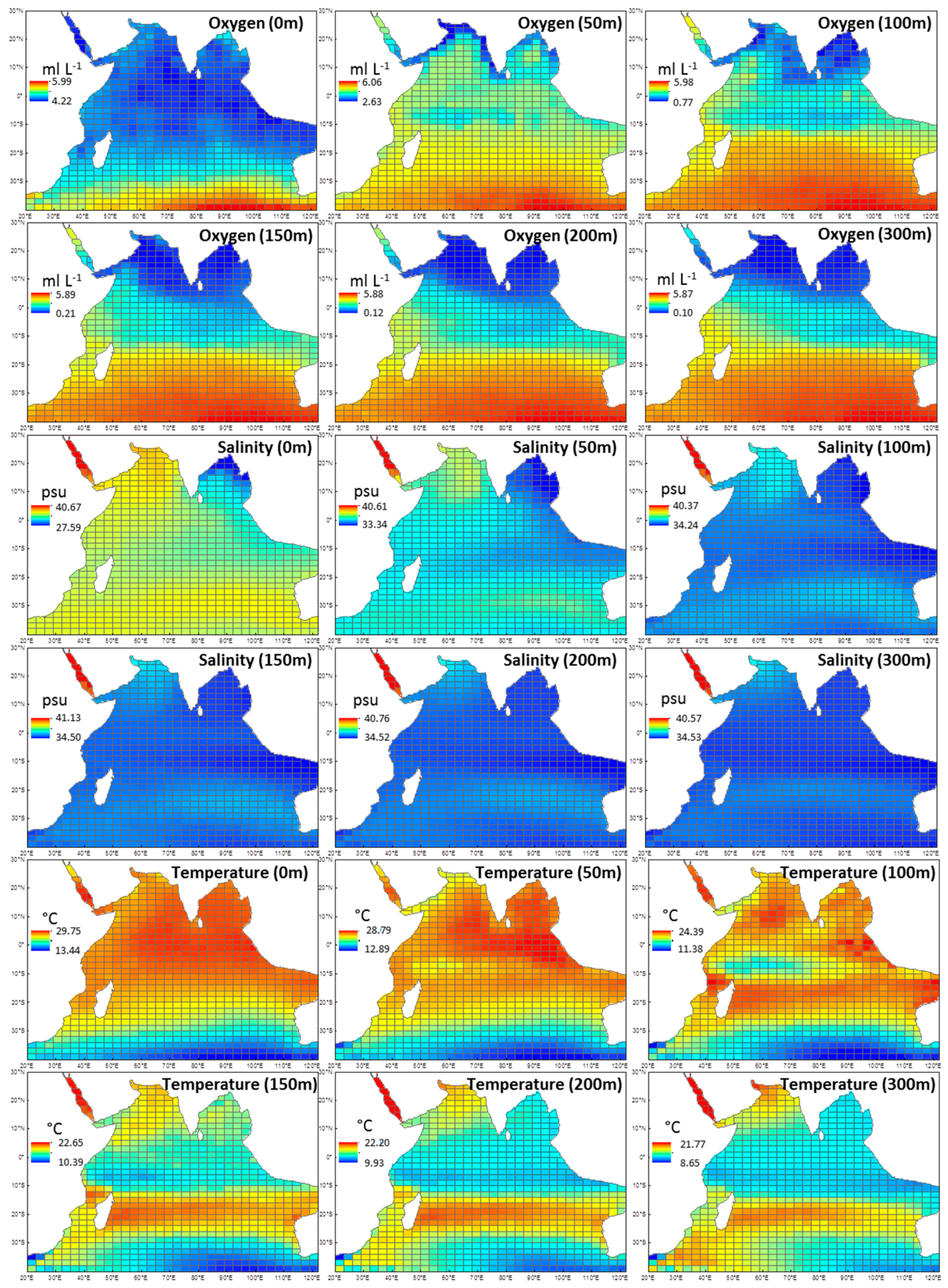
As euphausiid records span back to the IIOE of the 1960s, long-term climatologies and data sets were sourced. Environmental data were obtained from the Commonwealth Scientific and Industrial Research Organisation (CSIRO) Atlas of Regional Seas and National Aeronautics and Space Administration (NASA) OceanColor online databases (Table 2). The environmental variables included in the models were temperature, dissolved oxygen, salinity and surface chlorophyll a. Data for temperature, salinity and oxygen were obtained from a number of depths (0, 50, 100, 150, 200, 300 m; Appendix 1), and then averaged to give one mean value for the 300-m water column. A maximum depth of 300 m was chosen because euphausiids migrate through the water column, and most of the studies included in this analysis collected euphausiids within this range, particularly data from the IIOE (0–200 m sampling depths). All explanatory variables were chosen in order to find the most parsimonious and biologically relevant model for euphausiids.
2.4. Statistical Modelling
Data exploration was carried out using R v3.1.1 software (R Foundation for Statistical Computing, Vienna, Austria) and data were inspected for independence, outliers, normality and collinearity of variables, following [57]. Cleveland dot plots and box plots were used to identify any outliers, and histograms were used to assess normality. Collinearity between two variables was assessed using scatterplots and the Pearson correlation coefficient, and if the correlation was >0.7, the variable most appropriate in relation to euphausiids was kept. A generalised additive model (GAM) was used to investigate the relationships between environmental variables and euphausiid species richness and AveTD. A GAM was chosen for its ability to describe non-linear data [58]. Models were constructed using the mgcv package in R v3.1.1 [59]. A Poisson distribution with a log link was chosen for species richness and a Gaussian distribution with identity link to improve residuals was chosen for AveTD. Thin plate regression spline smoothers were applied to any non-linear variables included in the GAM model, as justified by the estimated degrees of freedom being >1 [60]. The estimated degrees of freedom were restricted to four for all models to avoid over-fitting of the data. Manual forward and backward stepwise selection after the GAM procedure was also performed to validate this selection based on minimisation of the Akaike information criteria (AIC) [61]. The importance of each explanatory variable in the models was determined by calculating the pseudo-R2 after sequentially removing one explanatory variable at a time from the model and comparing the change in the residual deviance from the full model. Model validation was assessed using scatter plots of residuals vs fitted values (equal variances), as well as residual histograms and quantile-quantile plots (normality) to identify any violations of the assumptions of the GAM.
3. Results
3.1. Euphausiid Species Richness in the Indian Ocean
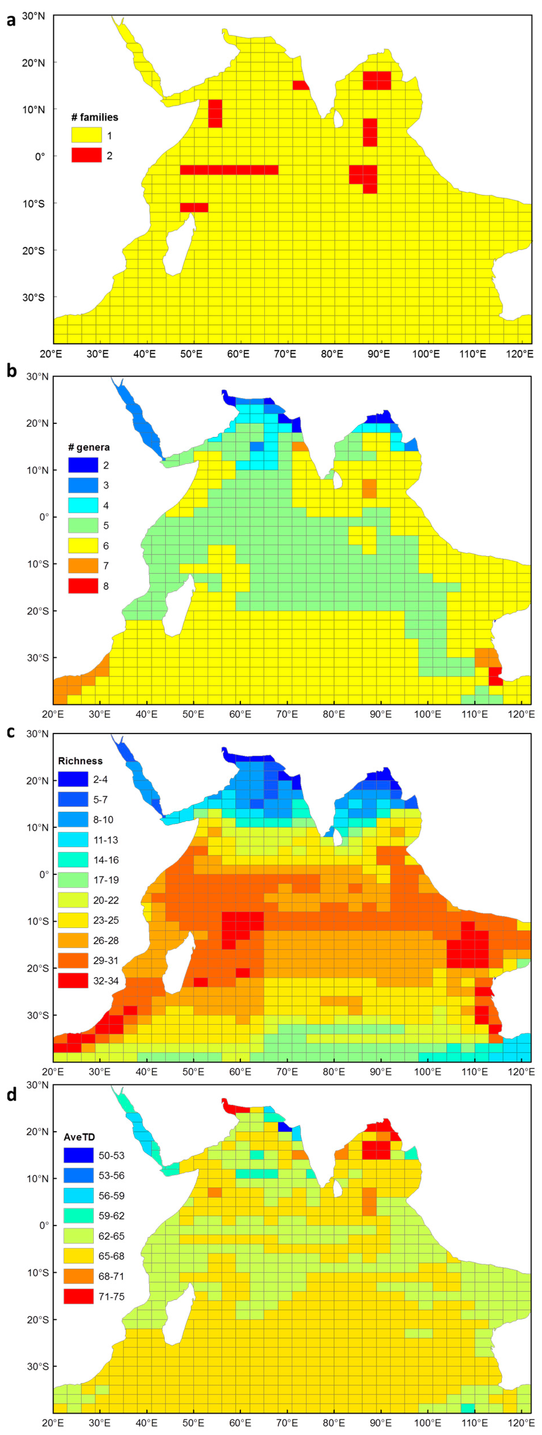
Fifty-six species of euphausiids occur within the Indian Ocean study area (Appendix 2). These include species from two families (Figure 1a), Bentheuphausiidae and Euphausiidae, and nine genera (Figure 1b) namely, Bentheuphausia, Euphausia, Nematoscelis, Nematobrachion, Nyctiphanes, Pseudeuphausia, Stylocheiron, Thysanoessa and Thysanopoda. Euphausia, Stylocheiron and Thysanopoda are the euphausiid genera with the most number of species, and these were well represented in the Indian Ocean, together accounting for 77% of the species recorded.
Species richness ranged between 2 and 34 species per cell (Figure 1c). Overall, there was a general decrease in species richness with increasing latitude, although there was an extension of high species richness in the southern hemisphere boundary currents i.e. Agulhas and Leeuwin Currents (Figure 1c). Species richness declined more rapidly with increasing latitude in the northern Indian Ocean, compared with the southern Indian Ocean. Areas with the highest species richness occurred within the Agulhas Current, Leeuwin Current, Indo-Australian basin and over the Mascarene Plateau. Areas of low species richness occurred in the northern Indian Ocean, most notably in the Arabian Sea, Bay of Bengal, Red Sea and the Persian Gulf. Relatively lower species richness also occurred off the southern coast of Australia.
3.2. Taxonomic Distinctness of Euphausiids in the Indian Ocean
AveTD ranged between 62 and 68 for most of the Indian Ocean (Figure 1d). A lower AveTD occurred across the tropics in comparison to the subtropical and temperate middle ocean basin of the southern Indian Ocean. The highest AveTD of euphausiids occurred where there was lowest species richness. The centre of the Bay of Bengal attained values between 71 and 75 and this was largely due to the presence of Benthueuphausia amblyops, from the monotypic family Bentheuphausiidae, and Pseudeuphausia latifrons, which is the only species of this genus found in the Indian Ocean. Additional areas of higher distinctness occurred in the Gulf of Oman and the northern extent of the Bay of Bengal. These localities were somewhat anomalous as only P. latifrons and Euphausia sibogae were recorded there, and the path length between these two species returned a relatively higher AveTD. The lowest AveTD occurred in the Red Sea (~56–62), and to the northeast of the Arabian Sea (~50–62). A randomisation test showed that all values of AveTD fell within the 95% probability limits of the expected mean for AveTD, which indicated that the euphausiid species sampled were representative of the Indian Ocean species pool.
3.3. The Indian Ocean Environment
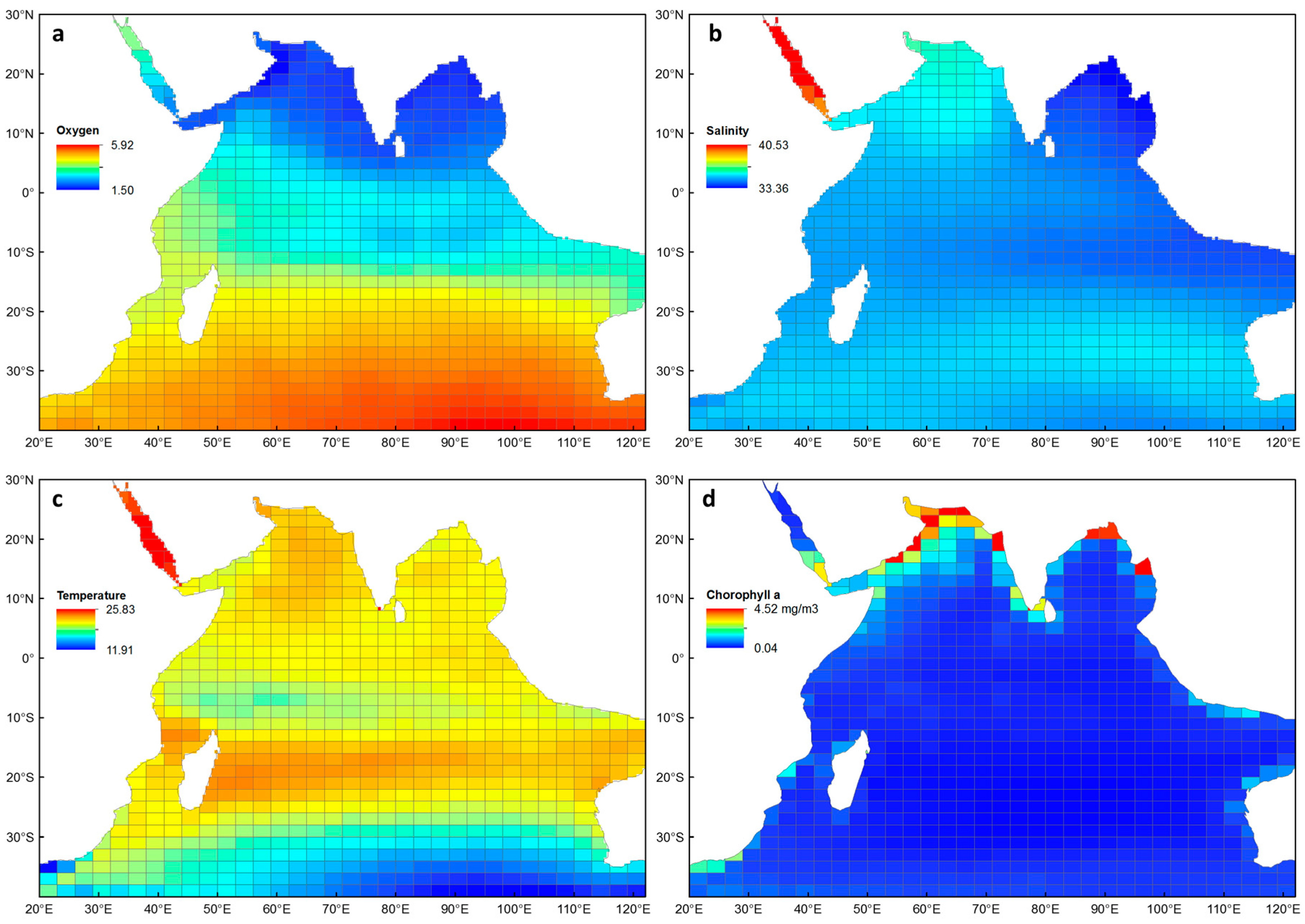
The four environmental explanatory variables that were correlated with euphausiid diversity are shown in Figure 2. There is a very clear gradient in average oxygen concentrations, from relatively low (1.5 ml L−1) in the northern Indian Ocean, to relatively high (5.9 ml L−1) in the southern Indian Ocean (Figure 2a). Average salinity was lowest in the Bay of Bengal (33.4 psu) and highest in the Red Sea, reaching a maximum of 40.4 psu (Figure 2b). Much of the Indian Ocean had average temperatures ranging between 19 and 21 °C, with a warmer band occurring around 20° S (Figure 2c), and a cooler band occurring between 0 and 10° S. The Red Sea had the highest average temperatures (> 23 °C), while cooler water was evident across the temperate zones of the southern Indian Ocean (< 14 °C). Average chlorophyll a was relatively low and ranged between 0.04–0.9 mg m−3 for most of the Indian Ocean (Figure 2d), with higher concentrations occurring along the coastlines, particularly in the Arabian Sea and Bay of Bengal (up to 4.52 mg m−3). The environmental data from cells in the Red Sea were removed from the GAMs due to being identified as outliers in the data set (n = 7).
3.4. Environmental Explanations of Euphausiid Zoogeography
3.4.1. Species Richness
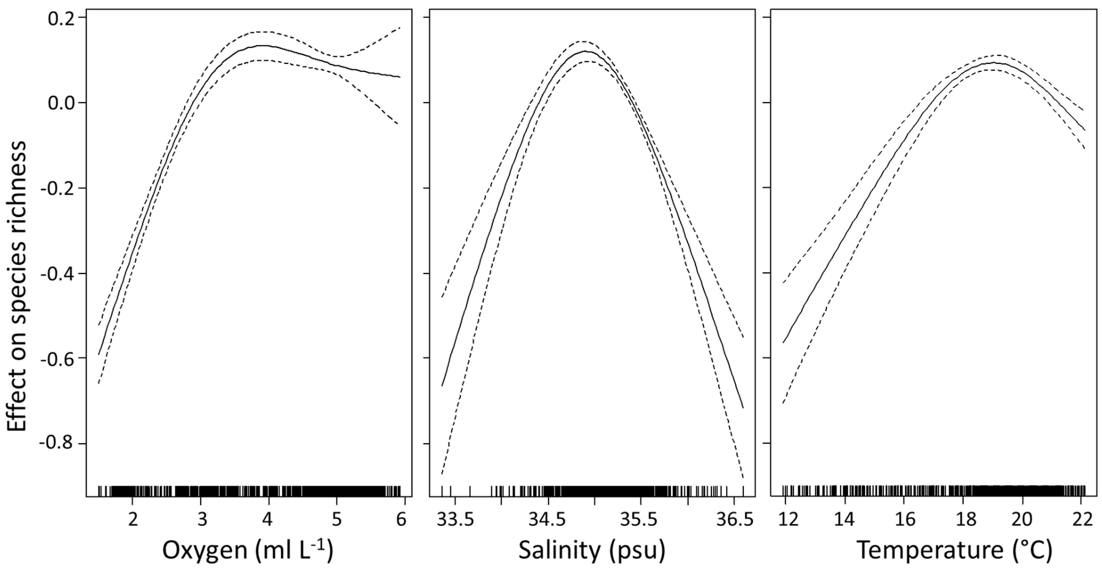
The GAM explained 78% of the variation in species richness (r2 = 0.783, p < 0.001, n = 701) (Table 3), and included all four explanatory variables (average temperature, salinity, dissolved oxygen and chlorophyll a). All variables were significant in the model (p < 0.001) (Table 4). All variables, except chlorophyll a, required the inclusion of a thin plate regression spline smoothing term. Chlorophyll a had a negative linear relationship with species richness (df = 1). Oxygen was the most important variable explaining the variance in species richness (Table 4). Species richness increased with greater oxygen levels until ~3.5 ml L−1 (Figure 3), thereafter richness remained relatively high and constant with any further rise in oxygen. Species richness increased with increasing salinity, with a clear peak occurring ~35 psu, after which species richness started to decline. Temperature had a similar effect, where richness increased until a temperature of ~19 °C, thereafter decreasing with further increases in temperature. The more linear relationship between species richness and chlorophyll a showed a decrease in richness with increasing chlorophyll a.
3.4.2. Average Taxonomic Distinctness
The GAM only explained 20% of the variation in AveTD of euphausiids (r2 = 0.19, p < 0.001, n = 701) (Table 3) and included the explanatory variables of average salinity, oxygen and chlorophyll a. Given this low explanatory power of the AveTD model, further exploration of the explanatory variables was not considered.
4. Discussion
Species richness and average taxonomic distinctness (AveTD) provided different perspectives on euphausiid diversity across the Indian Ocean. Species richness was generally higher in the tropics, and was extended southwards by boundary currents [55,62,63]. Conversely, AveTD was relatively uniform across the basin, reflecting the dominance by a single euphausiid family and a few genera. The unique environment of the northern Indian Ocean, most notably the low dissolved oxygen and salinity, were significantly correlated with the patterns observed for species richness.
The number of species occurring in the Indian Ocean (56) is less compared to values for the Atlantic Ocean (> 60) and Pacific Ocean (~ 81) [1,7,8,11,12]. There has been speculation that the high number of euphausiid species in the Pacific may be attributable to the older age and larger area encompassed by this ocean [11], some 32% of the earth’s surface. The Indian Ocean contains about 65% of the world’s species of euphausiids and this may be attributable, in part, to species entering the Indian Ocean from the more species rich Pacific Ocean via the Indonesian Throughflow [1,9].
Euphausiids are very low in diversity, in terms of total known species (86), compared to other orders from the class Malacostraca, such as Decapoda (>14,500 extant species) [64]. Most euphausiid species and their distributions are known [1,7,9,11,12,31], which would lessen the issue of sampling effort in comparison to more species-rich taxa that are relatively unknown. While future genetic differentiation of euphausiids may increase the number of species currently known [65], differentiation at the family level seems less likely. All but one species of euphausiid are attributed to the family Euphausiidae [6]. Any new species discovered would likely belong to this dominant family thus the pathway lengths would not be increased and taxonomic distinctness of euphausiids would remain similar. Bentheuphausia amblyops is from the monotypic family Bentheuphausiidae, and although AveTD converges on an average of all species pairs in the sample, the presence of B. amblyops in a sample increased the AveTD due to a longer path length through the classification tree. Bentheuphausia amblyops has a wide distribution throughout the Pacific and Atlantic Oceans, and thus, it is likely that this species occurs more widely in the Indian Ocean. However, due to its deep vertical distribution range (500–2000+ m) [7], the collection of this euphausiid may prove more difficult.
The northern Indian Ocean, particularly the Arabian Sea and Bay of Bengal, was different from the rest of the Indian Ocean in terms of species richness and environmental variables. These regions are known oxygen minimum zones [23,24,66], and as evident in the GAM, contributed to low euphausiid species richness. Similarly, a lower species richness of euphausiids occurs in the eastern Pacific Ocean [11], which has well-known oxygen minimum zones [67]. Bentheuphausia amblyops is usually found below 500 m [7], and has been found at the lower oxyclines in the Costa Rica Dome [68]. Euphausia sibogae has also been reported to tolerate oxygen minimum zones in the northern Indian Ocean, typically occurring around 300–400 m during the day, but migrating to the surface waters at night [7,9]. This behaviour is likely in response to such factors as predator avoidance, metabolic advantage and/or niche partitioning [23,69,70].
Salinity was also an important variable explaining some of the variation in species richness across the Indian Ocean. The lowest salinity was recorded from the Bay of Bengal, which receives a large freshwater influx from the rivers draining the Indian subcontinent and Southeast Asia [71], and this area corresponded with the lowest species richness of euphausiids. Euphausiid species richness modelled from the Pacific Ocean also found salinity to be a significant explanatory variable with high salinity correlated with high euphausiid richness, particularly in the subtropical gyres [11]. Species richness was highest for salinities of ~35 psu, which occurred across the majority of the Indian Ocean basin.
A latitudinal gradient in species richness is a widely observed pattern for a number of marine taxa [72,73], and is often strongly correlated with surface temperature [10,74]. For the Indian Ocean, high species richness of euphausiids was found in the tropics south of the equator (0–20° S) and was extended further south along the boundaries by transport in the Agulhas and Leeuwin Currents. However, in this study, the correlation between temperature and species richness, although significant, was relatively weak. The strength of the temperature and species richness relationship was likely inhibited by the confounding effect of the oxygen minimum zones in the northern Indian Ocean, creating lower species richness than would usually occur at tropical latitudes, due to the intolerance to low oxygen by many species [75]. Further, the presence of the cooler temperatures across the Seychelles–Chagos thermocline ridge (0–10° S) possibly contributed to the overall weakness of this relationship [76]. In contrast, the latitudinal gradients in euphausiids are clearly evident in the Atlantic Ocean [12] and Pacific Ocean [11], although gradients were investigated over a wider latitudinal range (60° S–60° N) than in this Indian Ocean study.
Chlorophyll a was a significant variable in the model for species richness and was highest where chlorophyll a concentrations were low. A negative relationship between chlorophyll a and species richness was also observed for the Atlantic Ocean [12] and it was suggested that a unimodal relationship existed between zooplankton and phytoplankton [77]. Contributing to this negative relationship in the Indian Ocean is the occurrence of high chlorophyll a in the Arabian Sea and Bay of Bengal, where oxygen minimum zones exist and fewer euphausiid species occur. Although a unimodal relationship could be occurring in the Indian Ocean as well, the effect of the oxygen minimum zones confounds the relationship between chlorophyll a and the species richness of euphausiids.
Patterns in species richness and taxonomic distinctness across the Indian Ocean are also a reflection of the holoplanktonic nature of euphausiids and ocean connectivity, with their distribution assisted via transport in currents [55,62,63]. One of the unique features of the Indian Ocean is its connectivity with the Pacific Ocean via the Indonesian Throughflow. The Indo-Australia Basin is a region with relatively high euphausiid species richness, which would be contributed to by the transport of species from the Pacific Ocean [9]. High species richness extended across the middle of the ocean basin in line with the South Equatorial Current, and this high species richness was extended southwards from the tropics via the Agulhas Current and Leeuwin Current. The Leeuwin Current attained richness values of up to 34 species in some cells and 37% of the world’s euphausiid species have been recorded in its waters [15,55,56]. Tropical species are also found as far south as 34° S, highlighting the Leeuwin Current as an effective transport route for euphausiids [55]. This is similar for the Agulhas Current, which contains ~45% of the world’s species. The species found in both current systems span eight genera from the Euphausiidae family, and most species are from the Euphausia, Stylocheiron and Thysanopoda genera. Given this, AveTD was not high, and is similar to the rest of the Indian Ocean.
5. Conclusion
This study has updated information on species richness and zoogeography for euphausiids in the Indian Ocean. It is the first study to apply taxonomic distinctness as a diversity measure across an entire ocean basin, but patterns in AveTD were not found to be particularly informative because of the dominance by one family (Euphausiidae). The results of this study suggest that oxygen and salinity are the most significant environmental variables influencing euphausiid species richness in the Indian Ocean, and reflects the unique oceanographic environment of the northern part of the basin.
Acknowledgements
Thanks are given to Susan Wijffels (CSIRO), for helpful discussion on the use of environmental data sets from the CSIRO Atlas of Regional Seas (CARS). The Ocean Biology Processing Group is credited for making chlorophyll a data available on the Ocean Color Web. Fiona Valesini and James Tweedley are thanked for useful statistical discussions. AS was funded by an Australian Postgraduate Scholarship from Murdoch University.
Author Contributions
A.S. and L.B conceived and designed the study; A.S. analysed the data; A.S. and L.B. wrote the paper.
Conflicts of Interest
The authors declare no conflict of interest.
Appendix A
Figure A1.
Derived environmental data from depths 0, 50, 100, 150, 200, 300 m that were used to obtain averages for oxygen (0–300 m), salinity (0–300 m), and temperature (0–300 m). Data was accessed from the Commonwealth Scientific and Industrial Research Organisation (CSIRO) Atlas of Regional Seas and represents annual means between 1950–2009.

Appendix B
List of the euphausiid species included in this study that had distribution records in the Indian Ocean between 30° N–40° S. Their frequency of occurrence in the 708 sampling cells is given as a percentage (in brackets).
| Euphausiid Species | ||
| Bentheuphausia amblyops (4%) | Nematobrachion flexipes (86%) | Stylocheiron microphthalma (47%) |
| Euphausia brevis (71%) | Nematobrachion sexspinosum (44%) | Stylocheiron robustum (34%) |
| Euphausia diomedae (65%) | Nematoscelis atlantica (55%) | Stylocheiron suhmi (58%) |
| Euphausia fallax (3%) | Nematoscelis gracilis (65%) | Thysanoessa gregaria (36%) |
| Euphausia hemigibba (69%) | Nematoscelis megalops (30%) | Thysanopoda acutifrons (15%) |
| Euphausia longirostris (1%) | Nematoscelis microps (75%) | Thysanopoda aequalis (59%) |
| Euphausia lucens (14%) | Nematoscelis tenella (87%) | Thysanopoda astylata (22%) |
| Euphausia mutica (65%) | Nyctiphanes australis (1%) | Thysanopoda cornuta (8%) |
| Euphausia paragibba (38%) | Nyctiphanes capensis (1%) | Thysanopoda cristata (58%) |
| Euphausia pseudogibba (15%) | Pseudeuphausia latifrons (31%) | Thysanopoda egregia (6%) |
| Euphausia recurva (40%) | Stylocheiron abbreviatum (91%) | Thysanopoda microphthalma (<1%) |
| Euphausia sanzoi (19%) | Stylocheiron affine (89%) | Thysanopoda minyops (1%) |
| Euphausia sibogae (32%) | Stylocheiron armatum (5%) | Thysanopoda monocantha (60%) |
| Euphausia similis (54%) | Stylocheiron carinatum (95%) | Thysanopoda obtusifrons (54%) |
| Euphausia similisarmata (16%) | Stylocheiron elongatum (85%) | Thysanopoda orientalis (76%) |
| Euphausia spinifera (25%) | Stylocheiron indicum (1%) | Thysanopoda pectinata (86%) |
| Euphausia tenera (61%) | Stylocheiron insulare (3%) | Thysanopoda spinicaudata (1%) |
| Euphausia vallentini (1%) | Stylocheiron longicorne (95%) | Thysanopoda tricuspidata (63%) |
| Nematobrachion boopis (89%) | Stylocheiron maximum (91%) | |
References
- Brinton, E. The distribution of Pacific euphausiids. Bull. Scripps Inst. Oceanogr. 1962, 8, 51–269. [Google Scholar]
- Mauchline, J.; Fisher, L.R. The biology of euphausiids. In Advances in Marine Biology; Russell, F.S., Younge, M., Eds.; Academic Press: London, UK, 1969; Volume 7, pp. 1–54. [Google Scholar]
- Kawamura, A. A review of food of balaenopterid whales. Sci. Rep. Whales Res. Inst. 1980, 32, 155–197. [Google Scholar]
- Hipfner, M.J. Euphausiids in the diet of a North Pacific seabird: Annual and seasonal variation and the role of ocean climate. Mar. Ecol. Prog. Ser. 2009, 390, 277–289. [Google Scholar] [CrossRef]
- Itoh, T.; Kemps, H.; Totterdell, J. Diet of young southern bluefin tuna Thunnus maccoyii in the southwestern coastal waters of Australia in summer. Fish. Sci. 2011, 77, 337–344. [Google Scholar]
- Baker, A.C.; Boden, P.; Brinton, E. A Practical Guide to Euphausiids of the World.; Natural History Museum: London, UK, 1990. [Google Scholar]
- Brinton, E.; Ohman, M.D.; Townsend, A.W.; Knight, M.D.; Bridgeman, A.L. Euphausiids of the World Ocean World Biodiversity Database CD-ROM Series; Springer: Paris, France, 2000. [Google Scholar]
- Gibbons, M. Pelagic biogeography of the South Atlantic Ocean. Mar. Biol. 1997, 129, 757–768. [Google Scholar] [CrossRef]
- Brinton, E. Euphausiids of southeast Asian waters. In Scientific Results of Marine Investigations of the South China Sea and the Gulf of Thailand; Naga Report; University of California, Scripps Institution of Oceanography: La Jolla, CA, USA, 1975; Volume 4, pp. 1–287. [Google Scholar]
- Tittensor, D.P.; Mora, C.; Jetz, W.; Lotze, H.K.; Ricard, D.; Berghe, E.V.; Worm, B. Global patterns and predictors of marine biodiversity across taxa. Nature 2010, 466, 1098–1101. [Google Scholar] [CrossRef] [PubMed]
- Letessier, T.B.; Cox, M.J.; Brierley, A.S. Drivers of variability in euphausiid species abundance throughout the Pacific Ocean. J. Plankton Res. 2011, 33, 1342–1357. [Google Scholar] [CrossRef]
- Letessier, T.B.; Cox, M.J.; Brierley, A.S. Drivers of euphausiid species abundance and numerical abundance in the Atlantic Ocean. Mar. Biol. 2009, 156, 2539–2553. [Google Scholar] [CrossRef]
- Brinton, E. Parameters relating to the distribution of planktonic organisms, especially euphausiids in the eastern tropical Pacific. Prog. Oceanogr. 1979, 8, 125–189. [Google Scholar] [CrossRef]
- Taki, K. Vertical distribution and diel migration of euphausiids from Oyashio Current to Kuroshio area off northeastern Japan. Plankton Benthos Res. 2008, 3, 27–35. [Google Scholar] [CrossRef]
- Sutton, A.L.; Beckley, L.E.; Holliday, D. Euphausiid assemblages in and around a developing anticyclonic Leeuwin Current eddy in the south-east Indian Ocean. J. R. Soc. West. Aust. 2015, 98, 9–18. [Google Scholar]
- Gibbons, M.; Barange, M.; Hutchings, L. Zoogeography and diversity of euphausiids around southern Africa. Mar. Biol. 1995, 123, 257–268. [Google Scholar] [CrossRef]
- Tarling, G.A.; Ward, P.; Sheader, M.; Williams, J.A.; Symon, C. Distribution patterns of macrozooplankton assemblages in the southwest Atlantic. Mar. Ecol. Prog. Ser. 1995, 120, 29–40. [Google Scholar] [CrossRef]
- Schott, F.A.; McCreary, J.P. The monsoon circulation in the Indian Ocean. Prog. Oceanogr. 2001, 51, 1–123. [Google Scholar] [CrossRef]
- Shankar, D.; Vinayachandran, P.N.; Unnikrishnan, A.S. The monsoon currents in the north Indian Ocean. Prog. Oceanogr. 2002, 52, 63–120. [Google Scholar] [CrossRef]
- Schott, F.A.; Xie, S.P.; McCreary, J.P. Indian Ocean circulation and climate variability. Rev. Geophys. 2009, 47. [Google Scholar] [CrossRef]
- Wiggert, J.D.; Murtugudde, R.G.; Christian, J.R. Annual ecosystem variability in the tropical Indian Ocean: Results of a coupled bio-physical ocean general circulation model. Deep-Sea Res. II 2006, 53, 644–676. [Google Scholar] [CrossRef]
- Naqvi, S.W.A.; Narvekar, P.V.; Desa, E. Coastal biogeochemical processes in the North Indian Ocean. In The Sea; Robinson, A., Brink, K., Eds.; Harvard University Press: Cambridge, MA, USA, 2006; Volume 14, pp. 723–780. [Google Scholar]
- Morrison, J.M.; Codispoti, L.A.; Smith, S.L.; Wishner, K.; Flagg, C.; Gardner, W.D.; Gaurin, S.; Naqvi, S.W.A.; Manghnani, V.; Prosperie, L.; Gundersen, J.S. The oxygen minimum zone in the Arabian Sea during 1995. Deep Sea Res. II 1999, 46, 1903–1931. [Google Scholar] [CrossRef]
- Naqvi, S.W.A.; Naik, H.; Jayakumar, A.; Pratihary, A.; Narvenkar, G.; Kurian, S.; Agnihotri, R.; Shailaja, M.S.; Narvekar, P.V. Seasonal anoxia over the western Indian continental shelf. In Indian Ocean Biogeochemical Processes and Ecological Variability; Wiggert, J.D., Hood, R.R., Naqvi, S.W.A., Smith, S.L., Brink, K.H., Eds.; American Geophysical Union: Washington, DC, USA, 2009; pp. 333–345. [Google Scholar]
- Gordon, A.L.; Fine, R.A. Pathways of water between the Pacific and Indian oceans in the Indonesian seas. Nature 1996, 379, 146–149. [Google Scholar] [CrossRef]
- Wijffels, S.; Meyers, G. An intersection of oceanic waveguides: Variability in the Indonesian Throughflow region. J. Phys. Oceanogr. 2004, 34, 1232–1253. [Google Scholar] [CrossRef]
- McCreary, J.P.; Miyama, T.; Furue, R.; Jensen, T.; Kang, H.W.; Bang, B.; Qu, T. Interactions between the Indonesian throughflow and circulations in the Indian and Pacific Oceans. Prog. Oceanogr. 2007, 75, 70–114. [Google Scholar] [CrossRef]
- Xu, J. Change of Indonesian Throughflow outflow in response to East Asian monsoon and ENSO activities since the last glacial. Sci. China Ser. D Earth Sci. 2014, 57, 791–801. [Google Scholar] [CrossRef]
- Meyers, G.; Bailey, R.J.; Worby, A.P. Geostrophic transport of Indonesian throughflow. Deep Sea Res. I 1995, 42, 1163–1174. [Google Scholar] [CrossRef]
- Domingues, C.M.; Maltrud, M.E.; Wijffels, S.E.; Church, J.A.; Tomczak, M. Simulated Lagrangian pathways between the Leeuwin Current System and the upper-ocean circulation of the southeast Indian Ocean. Deep Sea Res. II 2007, 54, 797–817. [Google Scholar] [CrossRef]
- Brinton, E.; Gopalakrishnan, K. The distribution of Indian Ocean euphausiids. In Biology of the Indian Ocean; Zeitzschel, B., Gerlach, S.A., Eds.; Springer Berlin Heidelberg: London, UK, 1973; pp. 357–382. [Google Scholar]
- Wilson, S.G.; Meekan, M.G.; Carleton, J.H.; Stewart, T.C.; Knott, B. Distribution, abundance and reproductive biology of Pseudeuphausia latifrons and other euphausiids on the southern North West Shelf, Western Australia. Mar. Biol. 2003, 142, 369–379. [Google Scholar] [CrossRef]
- Gallienne, C.P.; Conway, D.V.P.; Robinson, J.; Naya, N.; William, J.S.; Lynch, T.; Meunier, S. Epipelagic mesozooplankton distribution and abundance over the Mascarene Plateau and Basin, south-western Indian Ocean. J. Mar. Biol. Assoc. UK 2004, 84, 1–8. [Google Scholar] [CrossRef]
- Jayalakshmi, K.J.; Jasmine, P.; Muraleedharan, K.R.; Prabhakaran, M.P.; Habeebrehman, H.; Jacob, J.; Achuthankutty, C.T. Aggregation of Euphausia sibogae during Summer Monsoon along the Southwest Coast of India. J. Mar. Biol. 2011, 2011, 1–12. [Google Scholar] [CrossRef]
- Brinton, E. Vertical migration and avoidance capability of euphausiids in the California Current. Limnol. Oceanogr. 1967, 12, 451–483. [Google Scholar] [CrossRef]
- Wiebe, P.H.; Boyd, S.H.; Davis, B.M.; Cox, J.L. Avoidance of towed nets by the euphausiid Nematoscelis megalops. Fish. Bull. 1982, 80, 75–91. [Google Scholar]
- Gotelli, N.J.; Colwell, R.K. Quantifying biodiversity: procedures and pitfalls in the measurement and comparison of species richness. Ecol. Lett. 2001, 4, 379–391. [Google Scholar] [CrossRef]
- Warwick, R.M.; Clarke, K.R. New “biodiversity” measures reveal a decrease in taxonomic distinctness with increasing stress. Mar. Ecol. Prog. Ser. 1995, 129, 301–305. [Google Scholar] [CrossRef]
- Tolimieri, N.; Anderson, M.J. Taxonomic distinctness of demersal fishes of the California Current: moving beyond simple measures of diversity for marine ecosystem-based management. PLoS ONE 2010, 5, e10653. [Google Scholar] [CrossRef] [PubMed]
- Tweedley, J.R.; Warwick, R.M.; Valesini, F.J.; Platell, M.E.; Potter, I.C. The use of benthic macroinvertebrates to establish a benchmark for evaluating the environmental quality of microtidal, temperate southern hemisphere estuaries. Mar. Pollut. Bull. 2012, 64, 1210–1221. [Google Scholar] [CrossRef] [PubMed]
- Clarke, K.R.; Warwick, R.M. A taxonomic distinctness index and its statistical properties. J. App. Ecol. 1998, 35, 523–531. [Google Scholar] [CrossRef]
- Clarke, K.R.; Warwick, R.M. Changes in Marine Communities: An Approach to Statistical Analysis and Interpretation; PRIMER-E Ltd.: Plymouth, UK, 2001. [Google Scholar]
- Clarke, K.R.; Gorley, R.N. PRIMER v7: User Manual/Tutorial; PRIMER-E Ltd.: Plymouth, UK, 2015. [Google Scholar]
- Clarke, K.R.; Warwick, R.M. The taxonomic distinctness measure of biodiversity: Weighting of step lengths between hierarchical levels. Mar. Ecol. Prog. Ser. 1999, 184, 21–29. [Google Scholar] [CrossRef]
- Taniguchi, A. Mysids and euphausiids in the eastern Indian Ocean with particular reference to invasion of species from the Banda Sea. J. Mar. Biol. Assoc. India 1974, 16, 349–357. [Google Scholar]
- Cassanova, B. Evolution spatiale et structurale des peuplements d’euphausiaces de l’Antarctique au Golfe d’Aden. Sci. Mar. 1980, 44, 377–394. [Google Scholar]
- Nair, S.R.; Nair, V.R.; Achuthankutty, C.T.; Madhupratap, M. Zooplankton composition and diversity in western Bay of Bengal. J. Plankton Res. 1981, 3, 493–508. [Google Scholar] [CrossRef]
- Mathew, K.J. The ecology of Euphausiacea along the southwest coast of India. J. Mar. Biol. Assoc. India 1985, 27, 138–157. [Google Scholar]
- Silas, E.G.; Mathew, K.J. Spatial distribution of Euphausiacea (Crustacea) in the southeastern Arabian Sea. J. Mar. Biol. Assoc. India 1986, 28, 1–21. [Google Scholar]
- Fatima, M. Euphausiids of Somalian waters and Gulf of Aden collected in S.W. Monsoon season. Pak. J. Sci. Ind. Res. 1987, 30, 935–937. [Google Scholar]
- Hirota, Y. Vertical distribution of euphausiids in the Western Pacific Ocean and the Eastern Indian Ocean. Bull. Jpn. Sea Reg. Fish. Res. Lab. 1987, 37, 175–224. [Google Scholar]
- Hitchcock, G.L.; Lane, P.; Smith, S.; Luo, J.; Ortner, P.B. Zooplankton spatial distribution on coastal waters of the northern Arabian Sea, August, 1995. Deep Sea Res. II 2002, 49, 2403–2423. [Google Scholar] [CrossRef]
- Mathew, K.J.; Sivan, G.; Krishnakumar, P.K.; Kuriakose, S. Euphausiids of the West Coast of India; Central Marine Fisheries Research Institute: Cochin, India, 2003; p. 149. [Google Scholar]
- Holliday, D.; Beckley, L.E.; Weller, E.; Sutton, A.L. Natural variability of macro-zooplankton and larval fishes off the Kimberley, north-western Australia: Preliminary findings. J. R. Soc. West. Aust. 2011, 94, 85–99. [Google Scholar]
- Sutton, A.L.; Beckley, L.E. Influence of the Leeuwin Current on the epipelagic euphausiid assemblages of the south-east Indian Ocean. Hydrobiologia 2016, 779, 193–207. [Google Scholar] [CrossRef]
- Sutton, A.L.; Beckley, L.E. Euphausiid assemblages of the oceanographically complex north-west marine bioregion of Australia. Mar. Fresh. Res. 2017. [Google Scholar] [CrossRef]
- Zuur, A.F.; Ieno, E.N.; Elphick, C.S. A protocol for data exploration to avoid common statistical problems. Methods Ecol. Evol. 2010, 1, 3–14. [Google Scholar] [CrossRef]
- Austin, M.P. Spatial prediction of species distribution: An interface between ecological theory and statistical modelling. Ecol. Model. 2002, 157, 101–118. [Google Scholar] [CrossRef]
- Wood, S.N. Generalised Additive Models, An Introduction with R, 2nd ed.; Chapman and Hall/CRC: Boca Raton, FL, USA, 2006; 392p. [Google Scholar]
- Zuur, A.F. A Beginner’s Guide to Generalised Additive Models with R; Highland Statistics Ltd.: Newburgh, UK, 2012; p. 194. [Google Scholar]
- Burnham, K.P.; Anderson, D.R. Multimodel inference—Understanding AIC and BIC in model selection. Sociol. Methods Res. 2004, 33, 261–304. [Google Scholar] [CrossRef]
- Swartzman, G.; Hickey, B.; Kosro, P.M.; Wilson, C. Poleward and equatorward currents in the Pacific Eastern Boundary Current in summer 1995 and 1998 and their relationship to the distribution of euphausiids. Deep Sea Res. II 2005, 52, 73–88. [Google Scholar] [CrossRef]
- Nicol, S. Krill, currents, and sea ice: Euphausia superba and its changing environment. Bioscience 2006, 56, 111. [Google Scholar] [CrossRef]
- De Grave, S.; Pentcheff, N.D.; Ahyong, S.T.; Chan, T.-Y.; Crandall, K.A.; Dworschak, P.C.; Felder, D.L.; Feldmann, R.M.; Fransen, C.H.J.M.; Goulding, L.Y.D.; et al. A classification of living and fossil genera of decapod crustaceans. Raffles Bull. Zool. 2009, 21, 1–109. [Google Scholar]
- Bucklin, A.; Wiebe, P.H.; Smolenack, A.B.M.; Copley, N.J.; Beaudet, J.G.; Bonner, K.G.; Farber-Lorda, J.; Pierson, J.J. DNA barcodes for species identification of euphausiids (Euphausiacea, Crustacea). J. Plankton Res. 2007, 29, 483–493. [Google Scholar]
- Hood, R.R.; Beckley, L.E.; Wiggert, J.D. Biogeochemical and ecological impacts of boundary currents in the Indian Ocean. Prog. Oceanogr. 2017. [Google Scholar] [CrossRef]
- Paulmier, A.; Ruiz-Pino, D. Oxygen minimum zones (OMZs) in the modern ocean. Prog. Oceanogr. 2009, 80, 113–128. [Google Scholar]
- Maas, A.E.; Frazer, S.H.; Outram, D.M.; Seibel, B.A.; Wishner, K.E. Fine-scale vertical distribution of macroplankton and micronekton in the Eastern Tropical North Pacific in association with an oxygen minimum zone. J. Plankton Res. 2014, 36, 1557–1575. [Google Scholar]
- Wishner, K.F.; Ashjian, C.J.; Gelfman, C.; Gowing, M.M.; Kann, L.; Levin, A.; Mullineaux, L.S.; Saltzman, J. Pelagic and benthic ecology of the lower interface of the Eastern Tropical Pacific oxygen minimum zone. Deep Sea Res. I 1995, 42, 93–115. [Google Scholar]
- Antezana, T. Species-specific patterns of diel migration into the oxygen minimum zone by euphausiids in the Humboldt Current ecosystem. Prog. Oceanogr. 2009, 83, 228–236. [Google Scholar]
- Vinayachandran, P.N.; Kurian, J. Hydrographic observations and model simulations of the Bay of Bengal freshwater plume. Deep Sea Res. I 2007, 54. [Google Scholar] [CrossRef]
- Willig, M.R.; Kaufman, D.M.; Stevens, R.D. Latitudinal gradients of biodiversity: Pattern, process, scale, and synthesis. Ann. Rev. Ecol. Evol. Syst. 2003, 34, 273–309. [Google Scholar]
- Hillebrand, H. On the generality of the latitudinal diversity gradient. Am. Nat. 2004, 163, 192–211. [Google Scholar] [PubMed]
- Fuhrman, J.A.; Steele, J.A.; Hewson, I.; Schwalbach, M.S.; Brown, M.V.; Green, J.L.; Brown, J.H. A latitudinal diversity gradient in planktonic marine bacteria. Proc. Natl. Acad. Sci. USA 2008, 105, 7774–7778. [Google Scholar] [PubMed]
- Sameoto, D.; Guglielmi, L.; Lewis, M.K. Day/night vertical distribution of euphausiids in the eastern tropical Pacific. Mar. Biol. 1987, 96, 235–245. [Google Scholar] [CrossRef]
- Vialard, J.; Duvel, J-P.; McPhaden, M.; Bouruet-Aubertot, P.; Ward, B.; Key, E.; Bourras, D.; Weller, R.; Minnett, P.; Weill, A.; et al. Cirene: Air sea interactions in the Seychelles-Chagos thermocline ridge region. Bull. Am. Met. Soc. 2009, 90, 45–61. [Google Scholar] [CrossRef]
- Irigoien, X.; Huisman, J.; Harris, R.P. Global biodiversity patterns of marine phytoplankton and zooplankton. Nature 2004, 429, 863–867. [Google Scholar] [CrossRef] [PubMed]
Figure 1.
Euphausiid diversity showing (a) number of families, (b) number of genera, (c) species richness and (d) average taxonomic distinctness (AveTD) for each sampling cell in the Indian Ocean, collated from published euphausiid records.
Figure 1.
Euphausiid diversity showing (a) number of families, (b) number of genera, (c) species richness and (d) average taxonomic distinctness (AveTD) for each sampling cell in the Indian Ocean, collated from published euphausiid records.

Figure 2.
Mean values (0–300 m depth) used in generalised additive models for species richness and average taxonomic distinctness, extracted to each sampling cell for the Indian Ocean: (a) oxygen (ml L−1), (b) salinity (psu), (c) temperature (°C) and (d) chlorophyll a (mg m−3).
Figure 2.
Mean values (0–300 m depth) used in generalised additive models for species richness and average taxonomic distinctness, extracted to each sampling cell for the Indian Ocean: (a) oxygen (ml L−1), (b) salinity (psu), (c) temperature (°C) and (d) chlorophyll a (mg m−3).

Figure 3.
Smoothed additive effects of average oxygen concentration, salinity and temperature on euphausiid species richness in the Indian Ocean. Zero on the vertical axis corresponds to no effect of the explanatory variable. Dotted lines indicate the 95% confidence limits and the vertical dashes at the bottom of the plots show the distribution of points included in the model.

Table 1.
Published records of euphausiid occurrence and distribution used to produce the species richness map for the Indian Ocean.
Table 1.
Published records of euphausiid occurrence and distribution used to produce the species richness map for the Indian Ocean.
| Published Source | Indian Ocean Region | Sampling Net; Mesh Size | Depth Range (m) | # Samples |
|---|---|---|---|---|
| [45] Taniguchi 1974 | Indo-Australian Basin | Indian Ocean standard net * (1 m2); 0.33 mm | 0–2976 | 164 |
| Norpac net (50 cm and 56cm diameter) | ||||
| [46] Cassanova 1980 | Western Indian Ocean | Indian Ocean standard net * (1 m2); 0.33 mm | 0–4000 | 88 |
| 200 cm long net (44–48.5 cm diameter); 0.30 mm | ||||
| [47] Nair et al. 1981 | Bay of Bengal | Indian Ocean standard net * (1 m2); 0.33 mm | 0–200 | 22 |
| [48] Mathew 1985 | Arabian Sea | Indian Ocean standard net * (1 m2); 0.33 mm | 0–150 | 182 |
| [49] Silas and Mathew 1986 | Arabian Sea | Indian Ocean standard net * (1 m2); 0.33 mm | 0–1300 | 312 |
| Isaacs Kidd Mid-water Trawl | ||||
| [50] Fatima 1987 | Somalia, Gulf of Aden | Indian Ocean standard net * (1m2); 0.33 mm | Unknown | 9 |
| [51] Hirota 1987 | Eastern Indian Ocean | Multi-depth sampling (MTD) net (56 cm diameter); 0.10 mm, 0.33 mm, 0.68 mm | 0–1000 | 52 |
| [16] Gibbons et al. 1995 # | Southern Africa | Several net types | Various | Various |
| [7] Brinton et al. 2000 # | Whole basin | Indian Ocean standard net * (1 m2); 0.33 mm | 0–200 | 1231 |
| Several net types | Various | |||
| [52] Hitchcock et al. 2002 | Arabian Sea | MOCNESS (1 m2); 0.153 mm | 0–1200 | 6 |
| [53] Mathew et al. 2003 | Arabian Sea | Bongo net (60 cm diameter); 0.33 mm | 0–150 | 493 |
| [32] Wilson et al. 2003 | Eastern Indian Ocean, NW shelf Australia | Light traps | 0–75 | 426 |
| [33] Galliene et al. 2004 | Southwest Indian Ocean | Conical net (40 cm diameter); 0.125 mm | 0–50 | 36 |
| [54] Holliday et al. 2011 | Kimberley, eastern Indian Ocean | Bongo net (50 cm diameter); 0.35 mm | 0–150 | 72 |
| [34] Jayalakshmi et al. 2011 | Arabian Sea | Multiple Plankton Net Sampler (0.25 m2); 0.20 mm | Mixed layer/thermocline | 9 |
| [15] Sutton et al. 2015 | Southeast Indian Ocean | EZ net (1 m2); 0.335 mm | 0–200 | 36 |
| [55] Sutton and Beckley 2016 | Southeast Indian Ocean | Bongo net (50 cm diameter); 0.355 mm | 0–150 | 26 |
| [56] Sutton and Beckley 2017 | Indo-Australian Basin | Bongo net (50 cm diameter); 0.355 mm | 0–150 | 108 |
* Most samples collected used Indian Ocean standard net; # presented data from a collection of published studies; MTD = Motoda net, MOCNESS = Multiple opening/closing net and environmental sensing system, EZ = Multiple opening/closing plankton net system.
Table 2.
The explanatory environmental variables sourced from online databases to investigate correlations with euphausiid species richness and taxonomic distinctness in the Indian Ocean using generalised additive models.
Table 2.
The explanatory environmental variables sourced from online databases to investigate correlations with euphausiid species richness and taxonomic distinctness in the Indian Ocean using generalised additive models.
| Variable | Unit | Source | Time Period | Resolution/Average |
|---|---|---|---|---|
| Average temperature (0–300 m) | °C | www.marine.csiro.au/atlas/ | 1950–2009 | 0.5° × 0.5°/annually |
| Average salinity (0–300 m) | psu | www.marine.csiro.au/atlas/ | 1950–2009 | 0.5° × 0.5°/annually |
| Average oxygen (0–300 m) | ml L−1 | www.marine.csiro.au/atlas/ | 1950–2009 | 0.5° × 0.5°/annually |
| Average surface chlorophyll a | mg m−3 | https://oceancolor.gsfc.nasa.gov | 2002–2013 | 1°/annually |
Table 3.
The generalised additive models (GAMs) used to explain euphausiid species richness and average taxonomic distinctness (AveTD) in the Indian Ocean. The most parsimonious model is shown for each diversity measure along with the deviance explained, adjusted r2, the significance of the model (p value) and the number of sampling cells included in the analysis. The s before parentheses indicates a smoothing term was used.
| GAM Model | % Deviance Explained | Adjusted r2 | p Value | n |
|---|---|---|---|---|
| Species richness ~ s(oxygen) + s(salinity) + s(temperature) + chlorophyll a | 78.3 | 0.783 | <0.001 | 701 |
| AveTD ~ s(oxygen) + s(salinity) + s(chlorophyll a) | 20.4 | 0.194 | <0.001 | 701 |
Table 4.
The significance of each environmental explanatory variable included in the generalised additive model (GAM) for species richness of euphausiids in the Indian Ocean. The estimated degrees of freedom (EDF), chi-squared value and the difference in the % deviance explained when each variable was removed from the full model are also shown.
| Variable | EDF | Chi-Squared | p Value | Difference in % Deviance Explained |
|---|---|---|---|---|
| Oxygen | 2.6 | 468.9 | <0.001 | 13.4 |
| Salinity | 2.8 | 140.3 | <0.001 | 4.4 |
| Temperature | 2.8 | 144.4 | <0.001 | 4.7 |
| Chlorophyll a | 1.0 | <0.001 | 0.8 |
© 2017 by the authors. Licensee MDPI, Basel, Switzerland. This article is an open access article distributed under the terms and conditions of the Creative Commons Attribution (CC BY) license (http://creativecommons.org/licenses/by/4.0/).
Share and Cite
MDPI and ACS Style
Sutton, A.L.; Beckley, L.E. Species Richness, Taxonomic Distinctness and Environmental Influences on Euphausiid Zoogeography in the Indian Ocean. Diversity 2017, 9, 23. https://doi.org/10.3390/d9020023
AMA Style
Sutton AL, Beckley LE. Species Richness, Taxonomic Distinctness and Environmental Influences on Euphausiid Zoogeography in the Indian Ocean. Diversity. 2017; 9(2):23. https://doi.org/10.3390/d9020023
Chicago/Turabian StyleSutton, Alicia L., and Lynnath E. Beckley. 2017. "Species Richness, Taxonomic Distinctness and Environmental Influences on Euphausiid Zoogeography in the Indian Ocean" Diversity 9, no. 2: 23. https://doi.org/10.3390/d9020023
Note that from the first issue of 2016, this journal uses article numbers instead of page numbers. See further details here.