Response Ant Colony Optimization of End Milling Surface Roughness

Abstract

Metal cutting processes are important due to increased consumer demands for quality metal cutting related products (more precise tolerances and better product surface roughness) that has driven the metal cutting industry to continuously improve quality control of metal cutting processes. This paper presents optimum surface roughness by using milling mould aluminium alloys (AA6061-T6) with Response Ant Colony Optimization (RACO). The approach is based on Response Surface Method (RSM) and Ant Colony Optimization (ACO). The main objectives to find the optimized parameters and the most dominant variables (cutting speed, feedrate, axial depth and radial depth). The first order model indicates that the feedrate is the most significant factor affecting surface roughness.

1. Introduction

Roughness plays an important role in determining how a real object will interact with its environment. Rough surfaces usually wear more quickly and have higher friction coefficients than smooth surfaces. Roughness is performance of a mechanical component, since irregularities in the surface may form nucleation soften a good prediction for cracks or corrosion. Although roughness is usually undesirable, it is difficult and expensive to control in manufacturing. Decreasing the roughness of a surface will usually exponentially increase its manufacturing costs. This often results in a trade-off between the manufacturing cost of a component and its performance in an application.

Planning of experiments through design of experiments has been used quite successfully in process optimization by Chen and Chen [1], Fung and Kang [2], Tang et al. [3], Vijian and Arunachalam [4], Yang [5] as well as Zhang et al. [6], etc. Four controlling factors including the cutting speed, the feed rate, the depth of cut, and the cutting fluid mixture ratios with three levels for each factor were selected. The Grey relational analysis is then applied to examine how the turning operation factors influence the quality targets of roughness average, roughness maximum and roundness. An optimal parameter combination was then obtained. Additionally, ANOVA was also utilized to examine the most significant factors for the turning process when the roughness average, roughness maximum and roundness are simultaneously considered.

Aslan et al., [7], using Design optimization of cutting parameters when turning hardened AISI 4140 steel (63 HRC) with Al₂O₃ + TiCN mixed ceramic tool used an orthogonal array and the analysis of variance (ANOVA) to optimization of cutting parameters. The flank wear (VB) and surface roughness (Ra) had investigated. Nalbant et al. [8] used a Taguchi method to find the optimal cutting parameters for surface roughness in turning operations of AISI 1030 steel bars using TiN coated tools. Three cutting parameters, namely, insert radius, feed rate, and depth of cut, are optimized with considerations of surface roughness, and so on. However, very few studies have been conducted to investigate roundness under different turning parameters. Additionally, proper application of cutting fluids as studied by Kalpakjian and Schmid, [9] and EI Baradie, [10], can increase productivity and reduce costs by allowing one to choose higher cutting speeds, higher feed rates and greater depths of cut. Effective application of cutting fluids can also increase tool life, decrease surface roughness, increase dimensional accuracy and decrease the amount of power consumed. Water-soluble (water-miscible) cutting fluids are primarily used for high speed machining operations because they have better cooling capabilities [10]. There fluids are also best for cooling machined parts to minimize thermal distortions. Water-soluble cutting fluids are mixed with water at different ratios depending on the machining operation. Therefore, the effect of water-soluble cutting fluids under different ratios was also considered in this study.

A recent investigation performed by Alauddin et al. [11] has revealed that when the cutting speed is increased, productivity can be maximised and, meanwhile, surface quality can be improved. According to Hasegawa et al. [12], surface finish can be characterised by various parameters such as average roughness (Ra), smoothening depth (Rp), root mean square (Rq) and maximum peak-to-valley height (Rt). The present study uses average roughness (Ra) for the characterisation of surface finish, since it is widely used in industry. By using factors such as cutting speed, feed rate and depth of cut, Hashmi and his coworkers [13,14] have developed surface roughness models and determined the cutting conditions for 190 BHN steel and Inconel 718. EI-Baradie [15] and Bandyopadhyay [16] have shown that by increasing the cutting speed, the productivity can be maximised and, at the same time, the surface quality can be improved. According to Gorlenko [17] and Thomas [18], surface finish can be characterised by various parameters. Numerous roughness height parameters such as average roughness (Ra), can be closely correlated. Mital and Mehta [19] have conducted a survey of the previously developed surface roughness prediction models and factors influencing the surface roughness. They have found that most of the surface roughness prediction models have been developed for steels.

2. Theoretical Background

2.1. Response Surface Method

This is a method for obtaining an approximate function using results of several numerical calculations to increase calculation efficiency and thereby implement design optimization. In the response surface method, design parameters are changed to formulate an approximate equation by the design of experiments method. An approximate sensitivity calculation of a multicrestedness problem can be performed using a convex continuous function and applied to optimization. The Box-Behnken Design is normally used when performing non-sequential experiments. That is, performing the experiment only once. These designs allow efficient estimation of the first and second–order coefficients. Because Box-Behnken designs have fewer design points, they are less expensive to run than central composite designs with the same number of factors. Box-Behnken designs do not have axial points, thus we can be sure that all design points fall within the safe operating zone. Box-Behnken designs also ensure that all factors are never set at their high levels simultaneously [20–22]. The proposed linear model correlating the responses and independent variables can be represented by the following expression:

$$y=\mathit{mCuttingspeed}+\mathit{nFeedrate}+\mathit{pAxialdepth}+C$$

(1)

where y is the response, C, m, n and p are the constants Equation (1) can be written in the Equation (2):

$$y={\beta }_0{x}_0+{\beta }_1{x}_1+{\beta }_2{x}_2+{\beta }_3{x}_3$$

(2)

where y is the response, x₀ = 1(dummy variable), x₁= cutting speed, x₂ = feedrate, and x₃ = axial depth. β₀ = C and β₁, β₂, and β₃, are the model parameters. The second-order model can be expressed as shown in Equation (3):

$$y^{″}={\beta }_0{x}_o+{\beta }_1{x}_1+{\beta }_2{x}_2+{\beta }_3{x}_3+{\beta }_{11}{x}^{2}1+{\beta }_{22}{x}^{2}2+{\beta }_{33}{x}^{2}3+{\beta }_{11}{x}_1{x}_2+{\beta }_{12}{x}_1{x}_3+{\beta }_{14}{x}_2{x}_3$$

(3)

2.2. Ant Colony Optimisation

Ant colony optimization algorithms are part of swarm intelligence, that is, the research field that studies algorithms inspired by the observation of the behaviour of swarms. Swarm intelligence algorithms are made up of simple individuals that cooperate through self-organization, that is, without any form of central control over the swarm members. A detailed overview of the self organization principles exploited by these algorithms, as well as examples from biology, can be found in [23].

One of the first researchers to investigate the social behaviour of insects was the French entomologist Pierre-Paul Grassé. In the 1940s and 1950s, he was observing the behaviour of termites in particular, the Bellicositermes natalensis and Cubitermes species. He discovered [24] that these insects are capable of reacting to what he called “significant stimuli,” signals that activate a genetically encoded reaction. He observed [24] that the effects of these reactions can act as new significant stimuli for both the insect that produced them and for the other insects in the colony.

Goss et al. [25] developed a model to explain the behaviour observed in the binary bridge experiment. Assuming that after t time units since the start of the experiment, m₁ ants had used the first bridge and m₂ the second one, the probability p₁ for the (m + 1)^th ant to choose the first bridge can be given by Equation (4):

$$P_{1(m+1)}=\frac{{(m_1+k)}^h}{{(m_1+k)}^h+{(m_2+k)}^h}$$

(4)

where parameters k and h are needed to fit the model to the experimental data. The probability that the same (m + 1)^th ant chooses the second bridge is P_2(m+1) = 1 − P_1(m+1). Monte Carlo simulations, run to test whether the model corresponds to the real data [10], showed very good fit for k ≈ 20 and h ≈ 2. This basic model, which explains the behaviour of real ants, may be used as an inspiration to design artificial ants that solve optimization problems defined in a similar way.

Ant colony optimization has been formalized into a combinatorial optimization metaheuristic by Dorigo et al. [26,27] and has since been used to tackle many combinatorial optimization problems (COPS). Given a COP, the first step for the application of ACO to its solution consists in defining an adequate model. This is then used to defined the central component of ACO: the pheromone model. The model of a COP may be defined as follows:

A model P = (S, Ω, f) of a COP consists of:

• a search space S defined over a finite set of discrete decision variables and a set Ω of constraints among the variables;
• an objective function f: $\mathrm{S}\to {𝒭}_0^{+}$ to be minimized

Ant System was the first ACO algorithm to be proposed in the literature [28–30]. Its main characteristic is that the pheromone values are updated by all the ants that have completed the tour. The pheromone update for τ_ij, that is, for edge joining cities i and j, is performed as follows [Equation (5)]:

$${\mathrm{T}}_{\text{ij}}\leftarrow (1-\rho ).{\mathrm{T}}_{\text{ij}}+{\sum }_{\mathrm{k}=1}^{\mathrm{m}}{\mathrm{\Delta }\mathrm{T}}_{\text{ij}}^{\mathrm{k}}$$

(5)

where ρ is the evaporation rate, m is the number of ants, and ${\mathrm{\Delta }\mathrm{T}}_{\text{ij}}^{\mathrm{k}}$ is the quantity of pheromone per unit length laid on edge (i, j) by the kth ant [28] as shown in Equation (6):

$${\mathrm{\Delta }\mathrm{T}}_{\text{ij}}^{\mathrm{k}}=\{\begin{array}{ll}\frac{Q}{L_k},& \mathit{if\; ant\; k\; used\; edge} (i,j) \mathit{in\; its\; tour}\\ 0,& \mathit{otherwise}\end{array}$$

(6)

where Q is a constant and L_k is the tour length of the kth ant.

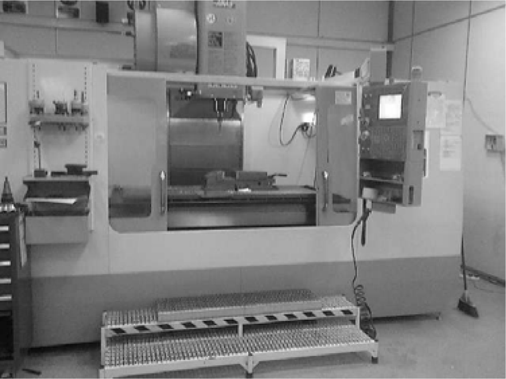
3. Experimental Setup

The 27 experiments were carried out on a 6-axes Haans machining centre as shown in Figure 1. A water soluble coolant was used in these experiments. Each experiment was stopped after 90 mm cutting length. For the surface roughness measurement surface roughness tester was used. Each experiment was repeated three times using a new cutting edge every time to obtain accurate readings of the surface roughness. The physical and mechanical properties of the workpiece are shown in

Table 1. Physical properties for workpiece.

Component	Al	Cr	Cu	Fe	Mg	Mn	Si	Ti	Zn
Wt %	95.8–98.6	0.04–0.35	0.15–0.4	Max 0.7	0.8–1.2	Max 0.15	0.4–0.8	Max 0.15	Max 0.25

and

Table 2. Design Parameters.

Cutting speed (m/min)	Feedrate (mm/rev)	Axial depth (mm)	Radial depth (mm)
140	0.15	0.10	5.0
140	0.15	0.15	3.5
100	0.15	0.15	5.0
140	0.15	0.15	3.5
180	0.15	0.20	3.5
180	0.15	0.15	2.0
100	0.20	0.15	3.5
140	0.15	0.15	3.5
180	0.15	0.15	5.0
100	0.15	0.20	3.5
140	0.20	0.10	3.5
180	0.10	0.15	3.5
140	0.15	0.20	2.0
180	0.15	0.10	3.5
140	0.10	0.15	2.0
140	0.15	0.20	5.0
100	0.15	0.10	3.5
140	0.20	0.15	2.0
100	0.15	0.15	2.0
140	0.20	0.15	5.0
140	0.10	0.10	3.5
140	0.20	0.20	3.5
140	0.15	0.10	2.0
100	0.10	0.15	3.5
180	0.20	0.15	3.5
140	0.10	0.20	3.5
140	0.10	0.15	5.0

. After the preliminary investigation, the suitable levels of the factors are used in the statistical software to deduce the design parameters for the aluminium alloy (AA6061-T6) as shown in

Table 3. Mechanical properties of the workpiece.

Hardness, Brinell	95
Hardness, Knoop	120
Hardness, Rockwell A	40
Hardness, Rockwell B	60
Hardness, Vickers	107
Ultimate Tensile Strength	310 MPa
Tensile Yield Strength	276 MPa
Elongation at Break	12 %
Elongation at Break	17 %
Modulus of Elasticity	68.9 GPa
Density	2.7 g/cc

. The lower and higher speed values selected are 100 m/s and 180 m/s, respectively. For the feed, the lower value is 0.1 mm/rev and the higher value is 0.2 mm/rev. For the axial depth, the higher value is 0.2 mm and the lower value is 0.1 mm and for the radial depth the higher value is 5 mm and lower value is 2 mm.

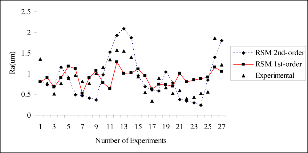
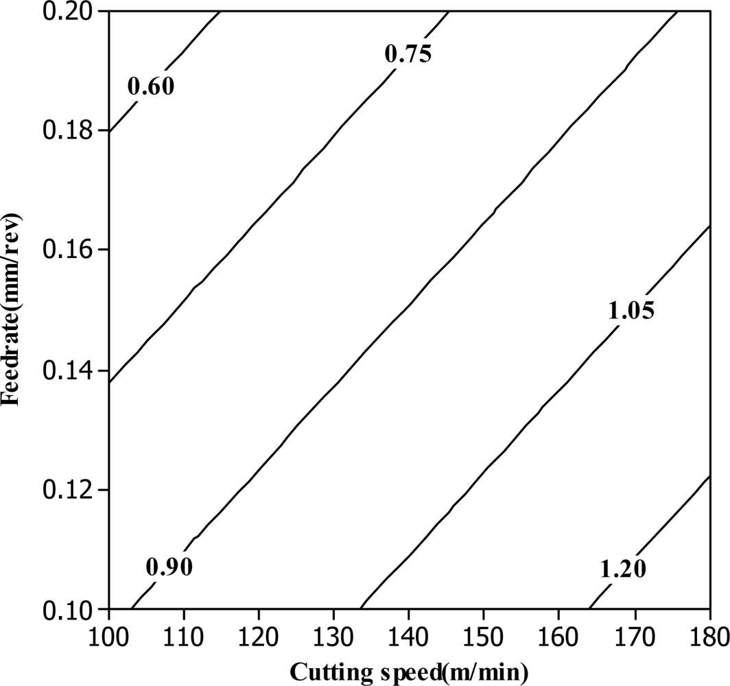
4. Results and Discussion

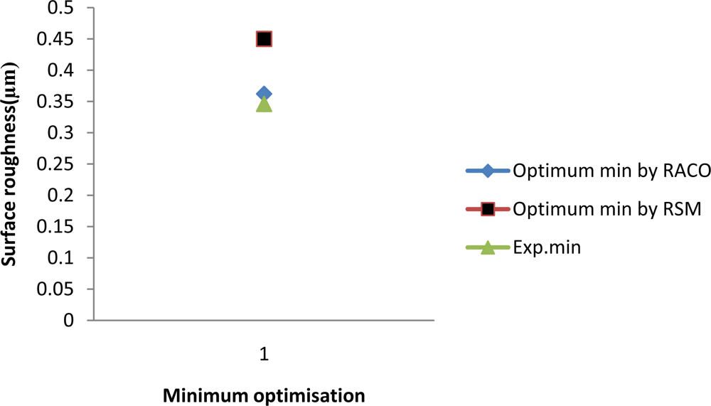
After conducting the first pass (one pass is equal to 90 mm length) of the 27 cutting experiments, the surface roughness readings are used to find the parameters appearing in the postulated first order model (Equation 1). In order to calculate these parameters, the least squares method is used with the aid of Minitab. The first-order linear equation used to predict the surface roughness is expressed by Equation 7:

$$R_a=0.5764+0.0049C_{\mathit{speed}}+3.5850f+1.5383a_{\mathit{depth}}+0.016r_{\mathit{depth}}$$

(7)

where the C_speed, f, a_depth and r_depth are the cutting speed, feed rate, axial depth and radial depth respectively.

Generally, reduction of cutting speed, axial depth of cut caused a larger surface roughness. On the other hand, the increase in feed rate and radial depth caused a slight reduction of surface roughness. The feed rate is the most dominant factor on the surface roughness, followed by the axial depth, cutting speed and radial depth, respectively. Hence, a better surface roughness is obtained with the combination of low cutting speed and axial depth, high feed rate and radial depth. Similar to the first-order model, by examining the coefficients of the second-order terms, the feedrate (f) has the most dominant effect on the surface roughness. After examining the experimental data, it can be seen that the contribution of cutting speed (C_speed) is the least significant. As seen from Figure 2, the predicted surface roughness using the second order RSM model is closely matched with the experimental results. It exhibits better agreement compared to those from the first-order RSM model. A contour plot of feed rate versus cutting speed for the first-order model is shown in Figure 3. It is clear that the relationship between the surface roughness and design variables can be obtained. The analysis of variance (ANOVA) for first order is tabulated in

Table 4. Analysis of variance for first-order equation.

Source	DOF	Seq. SS	Adj. SS	Adj. MS	F	P
Regression	4	0.9309	0.9309	0.2327	0.78	0.552
Linear	4	0.9309	0.9309	0.2327	0.78	0.552
Residual Error	22	6.5937	6.5937	0.2997
Lack-of-Fit	20	6.3151	6.3151	0.3158	2.27	0.351
Pure Error	2	0.2786	0.2786	0.1393
Total	26	7.5246

. It indicates that the model is adequate as the P-value of the lack-of-fit is not significant (>0.05).

5. Test Validation

The optimised surface roughness model is tested with experimental results. The predicted minimum surface roughness using optimised surface roughness model by RACO are compared with the measured surface roughness and these results are reported in Figure 4. The validation experiment is performed in the same machining environment as the training experiment. The errors of surface roughness obtained by optimised min surface roughness model are 4.65%. The optimum cutting parameters for minimum surface roughness are cutting speed 100 m/min; feed rate 0.2 mm/rev, axial depth 0.1 mm and radial depth 5 mm. On the other hand, the optimisation by RSM is 0.45 μm [31].

6. Conclusions

This research illustrates the machining of aluminium alloy (AA6061-T6) with end-milling methods and predicting their subsequent surface roughness. There is becoming a need for investigating the machining of various types of aluminium and their surface roughness, which in turn can be useful in developing more cost effective personalised products. The authors have shown the use of RACO to formulate an optimised minimum surface roughness prediction model for end machining of AA6061-T6. This prediction model is tested on the validation experimental and the error analysis of the prediction result with the measured results is estimated at 4.65% for minimum surface roughness which is small and shows the efficacy of the prediction model. Finally, the simulation results show that ACO combine with RSM can be very successively used for reduction of the effort and time required. This means that it can solve many problems that have mathematical and time constraints.

References and Notes

1. Chen, D.C.; Chen, C.F. Use of Taguchi method to study a robust design for the sectioned beams curvature during rolling. J. Mater. Proc. Tech 2007, 190, 130–137. [Google Scholar]
2. Fung, C.P.; Kang, P.C. Multi-response optimization in friction properties of PBT composites using Taguchi method and principle component analysis. J. Mater. Proc. Tech 2005, 170, 602–610. [Google Scholar]
3. Tang, S.H.; Tan, V.J.; Sapuan, S.M.; Sulaiman, S.; Ismail, N.; Samin, R. The use of Taguchi method in the design of plastic injection mould for reducing warpage. J. Mater. Proc. Tech 2007, 182, 418–426. [Google Scholar]
4. Vijian, P.; Arunachalam, V.P. Optimization of squeeze cast parameters of LM6 aluminium alloy for surface roughness using Taguchimethod. J. Mater. Proc. Tech 2006, 180, 161–166. [Google Scholar]
5. Yang, L.J. The effect of specimen thickness on the hardness of plasma surface hardened ASSAB 760 steel specimens. J. Mater. Proc. Tech 2007, 185, 113–119. [Google Scholar]
6. Zhang, J.Z.; Chen, J.C.; Kirby, E.D. Surface roughness optimization in a end-milling operation using the Taguchi design method. J. Mater. Proc. Tech 2007, 184, 233–239. [Google Scholar]
7. Aslan, E.; Camuscu, N.; Birgoren, B. Design optimization of cutting parameters when turning hardened AISI 4140 steel (63 HRC) with Al2O3 + TiCN mixed ceramic tool. Mater. Des 2007, 28, 1618–1622. [Google Scholar]
8. Nalbant, M.; Gokkaya, H.; Sur, G. Application of Taguchi method in the optimization of cutting parameters for surface roughness in turning. Mater. Des 2007, 28, 1379–1385. [Google Scholar]
9. Kalpakjian, S.; Schmid, S.R. Manufacturing Engineering and Technology, International, 4th ed; Prentice Hall: Upper Saddle River, NJ, USA, 2001; pp. 536–681. [Google Scholar]
10. EI Baradie, M.A. Cutting fluids: part I characterization. J. Mat. Proc. Tech 1996, 56, 786–797. [Google Scholar]
11. Alauddin, M.; EL Baradie, M.A.; Hashmi, M.S.J. Prediction of tool life in end milling by response surface methodology. J. Mater. Proc. Tech 1997, 71, 456–465. [Google Scholar]
12. Hasegawa, M.; Seireg, A.; Lindberg, R.A. Surface roughness model for turning. Tribol. Int 1976, 6, 285–289. [Google Scholar]
13. Alauddin, M.; El Baradie, M.A.; Hashmi, M.S.J. Computer-aided analysis of a surface-roughness model for end milling. J. Mat. Proc. Tech 1995, 55, 123–127. [Google Scholar]
14. Alauddin, M.; El Baradie, M.A.; Hashmi, M.S.J. Optimization of surface finish in end milling Inconel 718. J. Mat. Proc. Tech 1996, 56, 54–65. [Google Scholar]
15. EI-Baradie, M.A. Surface roughness model for turning grey cast iron 1154 BHN. Proc. IMechE 1993, 207, 43–54. [Google Scholar]
16. Bandyopadhyay, B.P.; Teo, E.H. Application of factorial design of experiment in high speed turning. Proc. Manuf. Int. Part 4, Advances in Materials & Automation, Atlanta, GA, USA, ASME, NY; 1990; pp. 3–8. [Google Scholar]
17. Gorlenko, O.A. Assessment of starface roughness parameters and their interdependence. Precis. Eng 1981, 3, 105–108. [Google Scholar]
18. Thomas, T.R. Characterisation of surface roughness. Precis. Eng 1981, 3, 2–8. [Google Scholar]
19. Mital, M. Mehta, Surface roughness prediction models for fine turning. Int. J. Pro. Re 1988, 26, 1861–1876. [Google Scholar]
20. Draper, N.R.; Smith, H. Applied Regression Analysis; Wiley: New York, NY, USA, 1981. [Google Scholar]
21. Box, G.E.P.; Draper, N.R. Empirical Model-Building and Response Surfaces; John Wiley & Sons Inc: New York, NY, USA, 1986; p. 669. [Google Scholar]
22. Box, G.E.P.; Behnken, D.W. Some new three level designs for the study of quantitative variables. Technometrics 1960, 2, 455–475. [Google Scholar]
23. Camazine, S.; Deneubourg, J.L.; Franks, N.; Sneyd, J.; Theraulaz, G.; Bonabeau, E. Self-Organization in Biological Systems; Princeton University Press: Princeton, NJ, USA, 2003. [Google Scholar]
24. Bonabeau, E.; Dorigo, M.; Theraulaz, G. Swarm Intelligence: From Natural to Artificial Systems; Oxford University Press: New York, NY, USA, 1999. [Google Scholar]
25. Grassé, P.P. La reconstruction du nid et les coordinations inter individuelles chez bellicositermes natalensis et cubitermes sp. La théorie de la stigmergie: essai d’interprétation du comportement des termites constructeurs. Insect. Soc 1959, 6, 41–48. [Google Scholar]
26. Dorigo, M.; Di Caro, G. The Ant Colony Optimization Meta-Heuristic. In New Ideas in Optimization; Corne, D., Dorigo, M., Glover, F., Eds.; McGraw-Hill: New York, NY, USA, 1999; p. 11. [Google Scholar]
27. Dorigo, M.; Di Caro, G.; Gambardella, L.M. Ant algorithms for discrete optimization. Artif. Life 1999, 5, 137–172. [Google Scholar]
28. Dorigo, M.; Maniezzo, V.; Colorni, A. Positive Feedback as a Search Strategy, Technical report 91-016; Dipartimento di Elettronica, Politecnico di Milano: Milan, Italy, 1991. [Google Scholar]
29. Dorigo, M. Optimization, Learning and Natural Algorithms, Ph.D. thesis,; Dipartimento di Elettronica, Politecnico di Milano: Milan, Italy, 1992.
30. Dorigo, M.; Maniezzo, V.; Colorni, A. Ant System: Optimization by a colony of cooperating agents. IEEE Trans. Syst. Man. Cybern 1996, 26, 29–41. [Google Scholar]
31. Kadirgama, K.; Noor, M.M.; Zuki, N.M.; Rahman, M.M.; Rejab, M.R.M.; Daud, R.; Abou-El-Hossein, K.A. Optimization of surface roughness in end milling on mould aluminium alloys (aa6061-t6) using response surface method and radian basis function network. Jordan J. Mech. Ind. Eng 2008, 2, 209–214. [Google Scholar]
Figure 1. Haans CNC milling with 6-axes.
Sensors 10 02054f1
Figure 2. Comparison between the experimental and predicted results.
Sensors 10 02054f2
Figure 3. Feed rate versus cutting speed contour plotted for first-order model.
Sensors 10 02054f3
Figure 4. Comparison of minimum optimised surface roughness with experimental and RSM.
Sensors 10 02054f4