SAR Image Segmentation Using Voronoi Tessellation and Bayesian Inference Applied to Dark Spot Feature Extraction

Abstract

This paper presents a new segmentation-based algorithm for oil spill feature extraction from Synthetic Aperture Radar (SAR) intensity images. The proposed algorithm combines a Voronoi tessellation, Bayesian inference and Markov Chain Monte Carlo (MCMC) scheme. The shape and distribution features of dark spots can be obtained by segmenting a scene covering an oil spill and/or look-alikes into two homogenous regions: dark spots and their marine surroundings. The proposed algorithm is applied simultaneously to several real SAR intensity images and simulated SAR intensity images which are used for accurate evaluation. The results show that the proposed algorithm can extract the shape and distribution parameters of dark spot areas, which are useful for recognizing oil spills in a further classification stage.

1. Introduction

Oil spills from operational discharges and ship accidents always have calamitous impacts on the marine environment and ecosystems, even with small oil coverage volumes. Remote sensing solutions using space-borne or airborne sensors are playing an increasingly important role in monitoring, tracking and measuring oil spills and are receiving much more attention from governments and organizations around the world. Compared to airborne sensors, satellite sensors, with their large extent observation, timely data available and all weather operation, are proven to be more suitable for monitoring oil spills in marine environments, whilst the latter can be easily used to identify polluters and oil spill types but are of limited use due to costs and weather conditions [1]. Currently, the commonly used SAR sensors for this purpose include RADARSAT-1/2, ENVISAT, ERS-1/2, and so on [1–4]. The detectability of oil spills by SAR sensors is based on the fact that oil slicks dampen the Bragg waves on the ocean surface and reduce the radar backscatter coefficient. Unfortunately, other physical phenomena, for example, low-wind areas, wind-shadow areas near coasts, rain cells, currents, upswelling zones, biogenic films, internal waves, and oceanic or atmospheric fronts, can also generate dark areas, known as look-alikes, in SAR images [5,6]. Another factor which influences the backscatter level and the visibility of oil slicks on the sea surface is the wind level. Oil slicks are visible only for a limited range of wind speeds [4,6].

Generally speaking, oil spill recognition includes three stages: dark spot detection, dark spot feature extraction and oil spill classification [6–8]. The work in this paper focuses on the feature extraction of detected dark spots [9]. The task at this stage involves defining and acquiring the features existing in SAR images, which can be efficiently used in the classification stage to distinguish oil spills from look-alikes. Commonly defined features for this purpose include the geometry and shape of the dark spot area, textures, contrast between dark spots and their surroundings, and dark spot contextual information [6,7,10,11]. In this paper, a new segmentation-based approach to extract the areas and outlines of dark regions and Gamma distribution parameters of dark regions in SAR images is presented. Many researchers have focused on their work on SAR segmentation issues. The segmentation algorithms for dark spot detection include threshold segmentation [12,13], edge extraction based segmentation, wavelets [14], and fuzzy clustering [15]. SAR images are highly speckled due to coherent processing [16]. The analysis of SAR images is usually required for region and statistics-based methodology in order to reduce the speckle effect. Following this idea, a new algorithm for segmentation of SAR images is considered, which is based on Voronoi tessellation [17] and Bayesian inference [18–21]. Voronoi tessellation has been widely used to characterize models for many natural phenomena or processes in crystallography, metallography, physics, astrophysics, biology, ecology, geology, geography, etc. [17] To segment a SAR intensity image, it is reasonable to approximate the homogenous regions in an SAR image by Voronoi polygons. The number of Voronoi polygons is assumed unknown. The intensities of pixels within a region defined by the polygons are distributed according to identical and independent Gamma distribution, with the parameters dependent on the homogenous region to which the polygon belongs. Following the Bayesian paradigm, the mathematical form of a posterior distribution is obtained up to an integrating constant. In order to simulate the posterior, a Markov Chain Monte Carlo (MCMC) scheme is developed, in which the move types are designed, including: (1) updating the distribution parameters; (2) updating the label for a polygon which indicates a homogenous region including the polygon; (3) updating the generating point and birth and death of generating points. For simplicity, a Maximum A Posteriori (MAP) criterion is used to obtain the optimal image segmentation and feature extraction.

The paper is organized as follows: Section 2 describes in detail the algorithm developed in this paper. In Section 3, the proposed algorithm is tested by several simulated 4-looks SAR intensity images and applied to RADARSAT-1 SAR intensity images for oil spill extraction. Finally, Section 4 contains concluding remarks and perspectives for further research.

2. Description of the Proposed Algorithm

2.1. Image Model

In a spatial statistic model, SAR backscatter energy can be characterized by a random field defined on a domain D⊂R², {Z(x, y); (x, y) ∈ D}, where Z(x, y) is a random function defined at the location (x, y). Under this framework, a SAR intensity image with n pixels can be viewed as the set of spatial samples from the random field at n discrete sites. A conventional sampling scheme is uniform sampling, in which regularly spaced positions are used. Therefore, a conventional digital SAR intensity image can be expressed by a set of random variables, that is, Z = {Z_i = Z(x_i, y_i); (x_i, y_i) ∈ D, i = 1, …, n} where i is the index of pixels, (x_i, y_i) is the location of pixel i, Z_i is the intensity variable of pixel i. The basic idea behind the segmentation algorithm for dark spot feature extraction lies in partitioning D into two homogenous regions D₁ and D₂ corresponding to the dark spot areas and its surroundings, respectively. To this end, D is partitioned into m sub-regions, that is, D = {P_j; j = 1,.., m}, where m is assumed unknown and with a prior distribution p(m), and a label L_j ∈ {1, 2} is assigned to the sub-region, say P_j, to indicate the homogenous region to which P_j belongs. The set of labels for all sub-regions forms a label field, that is, L = {L_j; j =1, …, m}. The intensities of pixels included in a sub-region are assumed to satisfy identical and independent Gamma distribution with parameters in terms of its label, so the joint probability distribution for the intensities of all pixels in the sub-region P_j, Z_j = {Z_i; (x_i, y_i) ∈ P_j}, can be written as:

$$p({\mathit{Z}}_j)=\text{∏}_{(x_i,y_i)\in P_j}\frac{{Z_i}^{{\alpha }_{{L_j}^{-1}}}}{\mathrm{\Gamma }({\alpha }_{L_j}){{\beta }_{L_j}}^{{\alpha }_{L_j}}}\cdot exp\left(-\frac{Z_i}{{\beta }_{L_j}}\right)$$

(1)

where (x_i, y_i) ∈ P_j, Γ(·) is Gamma function, α and β are the shape and scale parameters of the Gamma distribution. Let Θ = {α₁, α₂, β₁, β₂} be the set of parameters for Gamma distributions corresponding to dark spill regions and its surroundings, respectively. For a flexible and convenient tessellation, the Voronoi tessellation [17,22] is used for partitioning D into sub-regions called Voronoi polygons. Those polygons are specified by m generating points located at (u_j, v_j) ∈ D, where (u_j, v_j) are assumed to be independently distributed on D with a probability density function p(u_j, v_j). Let G = {(u_j, v_j) ∈ D; j = 1, …, m} denotes the set of all generating points. Given G, the Voronoi tessellation partitions D into a set of polygons, that is, D = {P_j; j = 1, …, m}, in which the jth Voronoi polygon P_j associated with the generating point (u_j, v_j) is comprised of the points nearest to (u_j, v_j) than to others in G, that is:

$$P_j=\left\{\left(x,y\right)\in \mathit{D};\left|\left(x,y\right)-\left(u_j,v_j\right)\right|<\underset{(u_{j^{\prime }},v_{j^{\prime }})\in G/(u_j,v_j)}{min}\left|(x,y)-(u_{j\text{'}},v_{j\text{'}})\right|\right\}$$

(2)

Given Θ, L, G and m, Z can be characterized by the likelihood function, p(Z |Θ, L, G, m), as follows:

$$p(\mathit{Z}|\mathit{\Theta },\mathit{L},\mathit{G},m)=\text{∏}_{j=1}^m\text{∏}_{(x_i,y_i)\in P_j}\frac{Z_i^{{\alpha }_{L_j}-1}}{\mathrm{\Gamma }({\alpha }_{L_j}){{\beta }_{L_j}}^{{\alpha }_{L_j}}}\cdot exp\left(-\frac{Z_i}{{\beta }_{L_j}}\right)$$

(3)

2.2. Bayesian Model

Using a Bayesian paradigm, the inference about parameters {Θ, L, G, m} given Z will be determined based on the joint posterior p (Z |Θ, L, G, m), which can be written as:

$$p(\mathit{\Theta },\mathit{L},\mathit{G},m\mid \mathit{Z})\propto p(\mathit{Z}\mid \mathit{\Theta },\mathit{L},\mathit{G},m)\cdot p(\mathit{\Theta })\cdot p(\mathit{L}\mid m)\cdot p(\mathit{G}\mid m)p(m)$$

(4)

where p(Z |Θ, L, G, m) is the likelihood defined by Equation (3)p(Θ) is the prior distribution for Gamma distribution parameters. Under the assumptions that all distribution parameters are independent, have p(Θ) = p(α₁)p(α₂)p(β₁)p(β₂). Furthermore, assume that the scale (resp. shape) parameters are drawn from Gaussian distribution with mean μ_β (resp. μ_α) and standard deviation σ_β (resp. σ_α), that is, β ∼ N(μ_βσ_β) (resp. α ∼ N(μ_α,σ_α)). As a result, the probability distribution function p(Θ) can be expressed as:

$$p(\Theta )=\text{∏}_{k=1}^2\frac{1}{\sqrt{2\pi }{\sigma }_{\alpha }}exp\left(-\frac{{({\alpha }_k-{\mu }_{\alpha })}^2}{2{{\sigma }_{\alpha }}^2}\right)\times \text{∏}_{k=1}^2\frac{1}{\sqrt{2\pi }{\sigma }_{\beta }}exp\left(-\frac{{({\beta }_k-{\mu }_{\beta })}^2}{2{{\sigma }_{\beta }}^2}\right)$$

(5)

p(L|m) is the prior distribution for label field which characterizes the relationship among labels. In this paper, the label field is modeled by a Markov Random Field [23], and an improved stationary Potts model [24] with 2 labels is used to model the prior distribution p(L|m). Two Voronoi polygons P_j and P_j' are neighbors if and only if they have a mutual boundary, denoted P_j ∼ P_j'. For a polygon P_j with label L_j, given its neighboring polygons NP_j = { P_j'; P_j' ∼ P_j }, the conditional distribution of L_j on {L_j'; P_j' ∈ NP_j } is expressed as:

$$p(L_j\mid L_{j\text{'}}\in N{P}_j)=\frac{exp\left\{b\text{∑}_{P_{j\text{'}}\in N{P}_j}t(L_j,L_{j\text{'}})\right\}}{\text{∑}_{L=1}^{2}exp\left\{b\text{∑}_{P_{j\prime }\in N{P}_j}t(L_j,L_{j\text{'}})\right\}}$$

(6)

where b > 0 is the constant to control the neighborhood dependences, and t (x, y) = 1, if x = y, otherwise t (x, y) = 0. As a result, the prior distribution p(L| m) can be written as:

$$p(\mathit{L}\mid m)=\text{∏}_{j=1}^{m}p(L_{j^{\prime }}\mid L_{j^{\prime }},P_{j^{\prime }}\in N{P}_j)$$

(7)

Assume that the locations of generating points (u_j, v_j) are independent and drawn from D uniformly, so the prior distribution p (G | m) is:

$$p(\mathit{G}\mid m)=\text{∏}_{j=1}^m\left(\frac{1}{\left|D\right|}\right)={\left(\frac{1}{\left|D\right|}\right)}^m$$

(8)

where |D| is the area of D. In this paper, the number of generating points m is assumed to satisfy a Poisson distribution with mean λ, that is:

$$p(m)=\frac{{\lambda }^m}{m!}exp(-\lambda )$$

(9)

The posterior distribution defined in Equation (4) can be derived according to the prior distributions of Equations (5)–(9) and image model in Equation (3) as follows:

$$\begin{array}{l}p(\mathit{\Theta },\mathit{L},\mathit{G},m\mid \mathit{Z})\propto \text{∏}_{j=1}^m\text{∏}_{(x_i,y_i)\in D_j}\frac{{Z_i}^{{\alpha }_{{L_j}^{-1}}}}{\mathrm{\Gamma }({\alpha }_{L_j}){{\beta }_{L_j}}^{{\alpha }_{L_j}}}exp\left(-\frac{z_i}{{\beta }_{L_j}}\right)\times \text{∏}_{k=1}^2\frac{1}{\sqrt{2\pi }{\sigma }_{\alpha }}exp\left(-\frac{{({\alpha }_k-{\mu }_{\alpha })}^2}{2{{\sigma }_{\alpha }}^2}\right)\times \\ \text{∏}_{k=1}^2\frac{1}{\sqrt{2\pi }{\sigma }_{\beta }}exp\left(-\frac{{({\beta }_k-{\mu }_{\beta })}^2}{2{{\sigma }_{\beta }}^2}\right)\times \text{∏}_{j=1}^m\frac{exp\left\{b\text{∑}_{P_{j\text{'}}\in N{P}_j}t(L_j,L_{j^{\prime }})\right\}}{\text{∑}_{l=1}^{2}exp\left\{b\text{∑}_{P_{j\text{'}\in N{P}_j}}t(L,L_{j\text{'}})\right\}}\times {\left(\frac{1}{\left|\mathit{D}\right|}\right)}^m\times \frac{{\lambda }^m}{m!}exp(-\lambda )\end{array}$$

(10)

2.3. Simulation

In order to segment an SAR intensity image, it is necessary to simulate it from the posterior distribution in Equation (10) and to estimate its parameters. Let Φ = (Θ, L, G, m) be parameter vectors. It is worthy to note that when m is variable, the dimension of the parameter vector Φ is varied. In this paper, Reversible Jump Markov Chain Monte Carlo (RJMCMC) algorithm [21] is used for this simulation. According to [21], at each iteration a new candidate Φ^* for Φ is proposed by an invertible deterministic function Φ^* = Φ^*(Φ, s) (assume that the dimension of Φ^* is higher than that of Φ). s is a random vector defined for accomplishing a transition from (Φ, s) to Φ^* with dimension matching, that is, |Φ| + |s| = |Φ^*|. The appropriate acceptance probability for the proposed transition is given by:

$$\alpha (\mathit{\Phi },{\mathit{\Phi }}^{*})=min\left\{1,\frac{p({\mathit{\Phi }}^{*}\mid \mathit{Z})r({\mathit{\Phi }}^{*})}{p(\mathit{\Phi }\mid Z)r(\mathit{\Phi })q(\text{s})}\left|\frac{\partial ({\mathit{\Phi }}^{*})}{\partial (\mathit{\Phi },s)}\right|\right\}$$

(11)

where q(s) is the density function of s and r(Φ^*) and r(Φ) are the probabilities of a given move type in the states Φ^* and Φ, respectively. The Jacobian |∂(Φ^*)/∂(Φ, s)| arises from the change of variable from (Φ, s) to Φ^*. The move types designed in this paper include: (1) updating Gamma distribution parameters; (2) updating the labels; (3) updating the positions of generating points; (4) birth or death of generating points.

Move 1: updating the gamma distribution parameters. Rewriting Θ = {Θ_k, k = 1, 2} where Θ_k = (α_k, β_k). Assume that the probability distributions for the proposals α_k^* and β_k^* are Gaussian distributions with means α_k and β_k, and standard deviations ε_αk and ε_βk, respectively, that is, α_k^* ∼ N (α_k., ε_αk) and β_k^* ∼ N (β_k, ε_βk). The acceptance probability for the proposals α_k^* and β_k^* can be obtained by:

$$a_1(\Theta k,{{\Theta }_k}^{*})=min\left\{1,\text{∏}_{j\in J_k}\frac{\text{∏}_{(x_i,y_i)\in P_j}p(Z_i\mid {{\Theta }_k}^{*})\times p({{\Theta }_k}^{*})}{\text{∏}_{(x_i,y_i)\in P_j}p(Z_i\mid {\Theta }_k)\times p({\Theta }_k)}\right\}$$

(12)

where J_k = {j', L_j' = k}, k∈ {1, 2}.

Move 2: updating labels. A label randomly drawn from the label fields L, say L_j, is updated by proposing a new label L_j^*, which is uniformly drawn from {1, 2}. The acceptance probability for L_j^* can be written as:

$$a_2(L_j,{L_j}^{*})=min\left\{1,\frac{\text{∏}_{(x_i,y_i)\in P_j}\frac{{Z_i}^{{\alpha }_{{L_j}^{*}}-1}}{\mathrm{\Gamma }({\alpha }_{{L_j}^{*}}){{\beta }_{{L_j}^{*}}}^{{\alpha }_{{L_j}^{*}}}}exp\left(-\frac{z_i}{{\beta }_{{L_j}^{*}}}\right)\times exp\left(2b\text{∑}_{P_{j\text{'}}\in N{P}_j}t({L_j}^{*},L_{j\text{'}})\right)}{\text{∏}_{(x_i,y_i)\in P_j}\frac{{Z_i}^{{\alpha }_{L_j}-1}}{\mathrm{\Gamma }({\alpha }_{L_j}){{\beta }_{L_j}}^{{\alpha }_{L_j}}}exp\left(-\frac{z_i}{{\beta }_{L_j}}\right)\times exp\left(2b\text{∑}_{P_{j\prime }\in N{P}_j}t(L_j,L_{j\text{'}})\right)}\right\}$$

(13)

Move 3: moving the position of generating points. One of generating points in G is drawn at random, say (u_j, v_j). A proposed position is (u_j^*, v_j^*) by drawing uniformly in P_j. The new proposed position gives rise to the local changes of P_j and its neighbour polygons to {P_j'^*, NP_j^*}. The acceptance probability for the move turns out to be:

$$a_3\left({(u_j,v_j)}_j,({u_j}^{*},{v_j}^{*})\right)=min\left\{1,\frac{\text{∏}_{P_{j\text{'}}\in \{P_j,N{P}_j^{*}\}}\text{∏}_{(x_i,y_i)\in P_{j\text{'}}*}\frac{Z_i^{{\alpha }_{L_j}-1}}{\mathrm{\Gamma }({\alpha }_{L_j}){{\beta }_{L_j}}^{{\alpha }_{L_j}}}exp\left(-\frac{z_i}{{\beta }_{L_j}}\right)}{\text{∏}_{P_{j\text{'}}\in \{P_j,N{P}_j\}}\text{∏}_{(x_i,y_i)\in P_{j\text{'}}}\frac{Z_i^{{\alpha }_{L_j}-1}}{\mathrm{\Gamma }({\alpha }_{L_j}){{\beta }_{L_j}}^{{\alpha }_{L_j}}}exp\left(-\frac{z_i}{{\beta }_{L_j}}\right)}\right\}$$

(14)

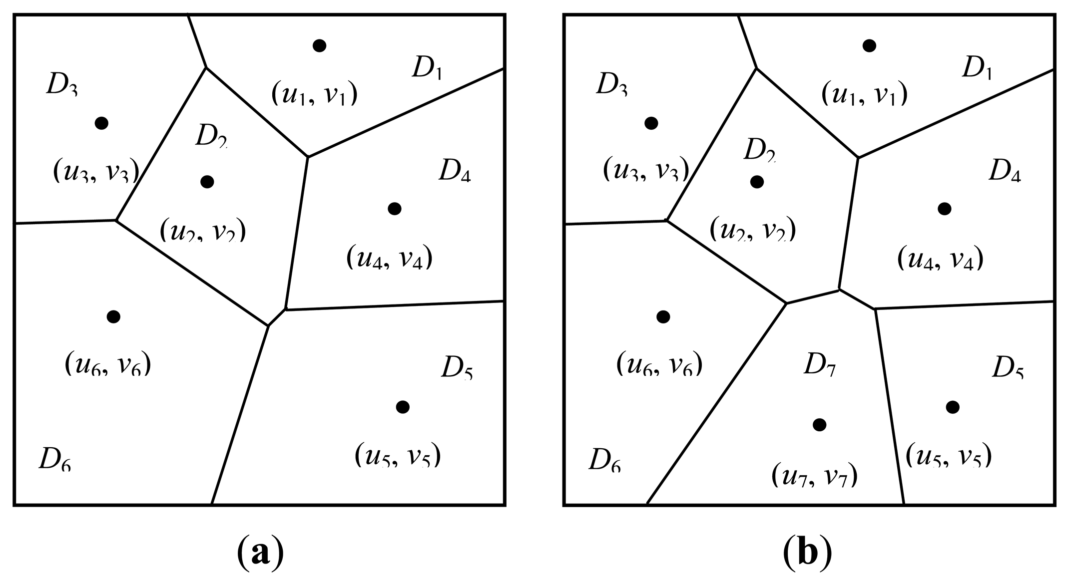
Move 4: birth or death of generating points. Suppose that the current number of generating points is m and let the probabilities of proposing a birth or death operation be b_m or d_m, respectively. Consider a birth operation which increases the number of generating points from m to m+1 and assume that the new generating point is labelled with m +1 and its location (u_m+1, v_m+1) is drawn uniformly from D. Let the polygon induced by (u_m+1, v_m+1) be P_m+1 and the set of labels of P_m+1's neighbor polygons is N_m+1. The Voronoi tessellation is modified by the addition of this generating point from P = {P₁, …, P_j', …, P_m} to P = {P₁, …, P_j'^*, …, P_m, P_m+1}. Figure 1 shows the modified Voronoi tessellation by the addition of a new generating point, in which the original tessellation have six generating points and they induce six polygons, see Figure 1a. By proposing a new generating point labelled 7, a new polygon is generated by it and denoted P₇. It can be observed from Figure 1b that the neighbors of P₇ include P₂, P₄, P₅ and P₆, that is, NP₇ = {2, 4, 5, 6}.

The new label L_m+1 for polygon P_m+1 is uniformly drawn from {1, 2}. It is evident that a birth or a death of generating point does not affect the Gamma distribution parameters in Θ. As a result, the parameter vector for the birth operation becomes Φ^* = (Θ, L^*, G^*, m+1) where L^* = (L₁, …, L_m, L_m+1), G^* = (G, (u_m+1, v_m+1)). The acceptance probability of the birth can be written as:

$$a_{4b}(\mathit{\Phi },{\mathit{\Phi }}^{*})=min\{1,R_{4b}\}$$

(15)

where:

$$\begin{array}{c}{R}_{4b}=\frac{p(\mathit{Z}\mid \mathit{\Theta },{\mathit{L}}^{*},{\mathit{G}}^{*},m+1)p(m+1)p({\mathit{L}}^{*}\mid m+1)p(\mathit{G}\mid m+1)r_{d_{m+1}}({\mathit{\Phi }}^{*})}{p(\mathit{Z}\mid \mathit{\Theta },\mathit{L},\mathit{G},m)p(m)p(\mathit{L}\mid m)p(\mathit{G}\mid m)r_{b_m}(\mathit{\Phi })q(s)}\left|\frac{\partial ({\mathit{\Phi }}^{*})}{\partial (\mathit{\Phi },s)}\right|\\ =\frac{\text{∏}_{P_j\in \{P_{m+1},N{P}_{m+1}\}}\text{∏}_{(x_i,y_i)\in P_j}\frac{Z_i^{{\alpha }_{L_j}-1}}{\mathrm{\Gamma }({\alpha }_{L_j}){{\beta }_{L_j}}^{{\alpha }_{L_j}}}exp(-\frac{z_i}{{\beta }_{L_j}})}{\text{∏}_{P_j\in N{P}_{m+1}}\text{∏}_{(x_i,y_i)\in P_j}\frac{Z_i^{{\alpha }_{L_j}-1}}{\mathrm{\Gamma }({\alpha }_{L_j}){{\beta }_{L_j}}^{{\alpha }_{L_j}}}exp\left(-\frac{z_i}{{\beta }_{L_j}}\right)}\times \frac{\text{∏}_{P_{j\in \{Pm+1,N{P}_{m+1}\}}}\frac{exp\left(b\text{∑}_{P_{j\text{'}\in N{P_j}^{*}}}t(L_j,L_{j\text{'}})\right)}{\text{∑}_{k=1}^{2}exp\left(b\text{∑}_{P_{j\text{'}\in N{P_j}^{*}}}t(k,L_{j\text{'}})\right)}}{\text{∏}_{P_j\in N{P}_{m+1}}\frac{exp\left(b\text{∑}_{P_{j\text{'}\in N{P}_j}}t(L_j,L_{j\text{'}})\right)}{\text{∑}_{l=1}^{2}exp\left(c\text{∑}_{P_{j\text{'}\in N{P}_j}}t(l,l_{j\text{'}})\right)}}\times \frac{\lambda }{{(m+1)}^2*k*|}\end{array}$$

(16)

where r_bm = b_m, r_dm+1 = d_m+1/(m+1), s = l_m+1. The acceptance probability of a death of generating point is:

$${\alpha }_{4d}(\mathit{\Phi },{\mathit{\Phi }}^{*})=min\{1,R_{4d}\},\text{and}{R}_{4d}={R_{4b}}^{-1}$$

(17)

For any given proposal with acceptance probability a, it is accepted if and only if a ≥ ψ, where ψ is drawn from [0, 1] uniformly, that is, ψ ∼ U (0, 1).

2.4. Optimization

To estimate the parameter vector Θ, its samples are drawn from the above posterior distribution in Equation (10) using the RJMCMC scheme. An MAP criterion is used to obtain the final segmentation, which is represented by the optimal label filed under maximizing the posterior. The MAP estimator is designed as:

$$\widehat{\mathit{L}}=arg\{max(p(\mathit{\Theta },\mathit{L},\mathit{G},m\mid \mathit{Z}))\}$$

(18)

3. Experimental Results and Discussion

To assess the accuracy of the proposed algorithm for extracting features of dark spots, two types of data, 4-looks SAR intensity images and simulated SAR intensity images which simulate 4-looks SAR intensity images, are used. It has been shown that multilook SAR intensity images can be modeled by Gamma distributions with fixed scale parameters, which are equal to the number of looks.

Table 1. Constants used in the experiment.

λ	b	μα	σα	μβ	σβ	εα	εβ	T
96	1	4	1	32	8	0.5	1	4,000

gives the constants used in this experiment, where λ is the mean of Poisson distribution from which the number of generating points is drawn. In a certain range, the value of λ does not affect the segmentation results. For simplicity, the correlation coefficient b is set as 1. The constants μ_α and μ_β are the means of shape parameter α and scale parameter β of the Gamma distributions in Equation (5), respectively, i.e., μ_α= E(α) and μ_β = E(β). Given a multi-look SAR image in which the intensities of pixels are characterized by Gamma distribution, α is equal to the number of its looks. In this paper, since α is considered as a random variable the value μ_α is set as the number of looks. For Gamma distribution with parameters α and β, the product of the two parameters, αβ, is equal to its mean. Then the value μ_α× μ_α = E(α)E(β) = E(αβ) (the last equation is true, since α and β are independent) is taken 128 = 256/2 (i.e., the midpoint of 256 grey levels) since the pixel intensities in a grey-scale image vary in the range of 0 and 255. ε_α and ε_β are the standard deviations for the proposal densities of the shape and scale parameters, that is, α^* ∼ N(α^t, ε_α) and β^* ∼ N(β^t, ε_β) where α^* and β^* is the proposals, α^t and β^t are the shape and scale parameters at t th iteration. They affect the sampling and the convergence of the algorithm under the MCMC scheme [18] suggested choosing the proposal variances so that the acceptance probability lies in the interval (0.3–0.7). However we have found that the proposal variances causing the acceptance probability around 0.1 still make the algorithm work well. T is the number of iterations. Usually, it depends on the complexity of the scene revealed in a SAR image and requirement of segmentation accuracy.

3.1. Simulated SAR Imagery

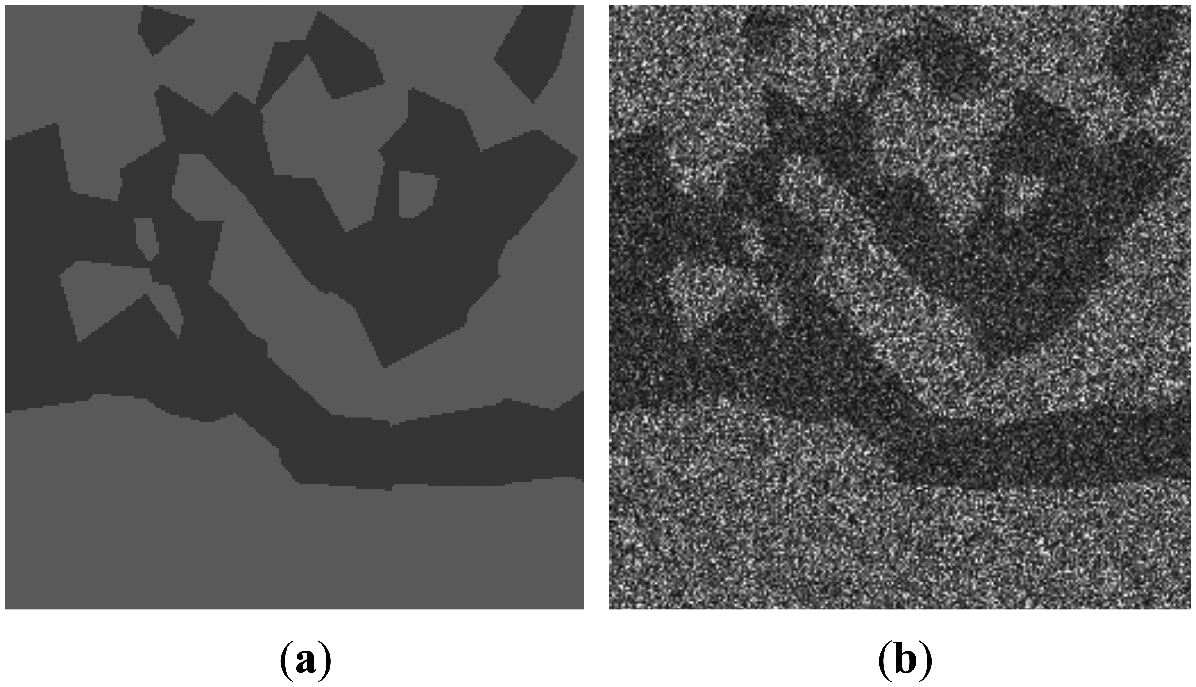
Figure 2 shows a simulated SAR image, which is generated based on the partition of a domain as shown in Figure 2a. In the simulated image in Figure 2b, the intensity values of pixels in each homogeneous region are drawn from gamma distributions with shape parameters equal to 4, and the scale parameters equal 18 and 28 for dark spill and background classes, respectively.

Table 2. Estimated model parameters and their errors.

	α	eα (%)	β	eβ(%)
C1	4.04	1.0	27.37	2.25
C2	3.95	1.25	18.56	3.11

gives the experimental results after 4,000 iterations of the proposed algorithm, including estimated distribution parameters α and β, and the estimation errors for the parameters (e%) corresponding to the optimal segmentations.

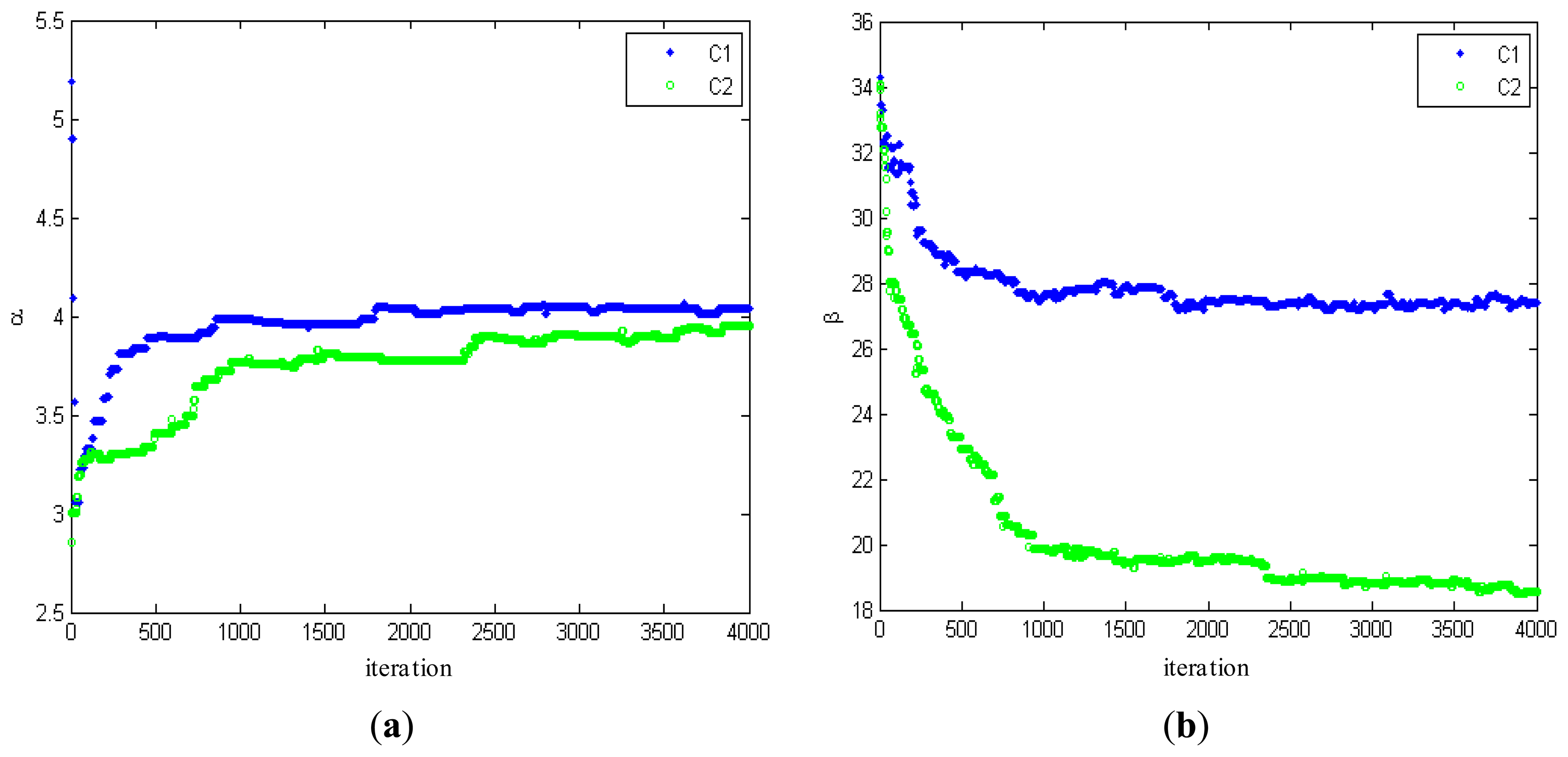
Figure 3 shows the changes of estimated parameters. From Figure 3, it can be seen that the estimated parameters converge to their stable values well at around 1,000 iterations, consistent with the results from the testing on a number of SAR intensity mages. In order to illustrate the convergence and stability of the proposed algorithm, 4,000 iterations are carried out.

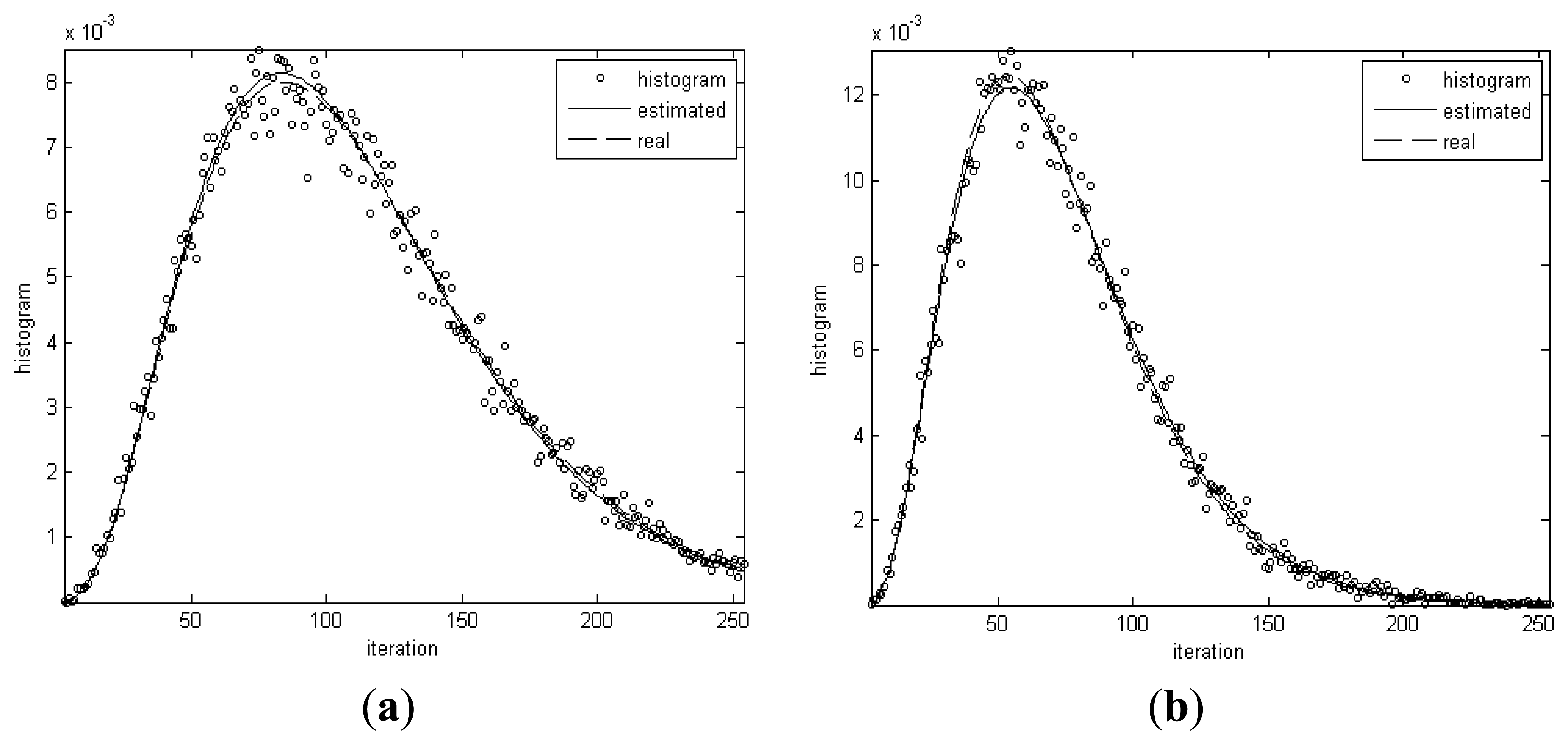
Figure 4 shows the histograms for the homogenous regions in the simulated image and distribution curves of Gamma distributions with real and estimated parameters, respectively. From Table 2 and Figure 4, it can be seen that the real and estimated values of distribution parameters for dark spot regions are very close. The maximum error is only 2.8%. The conclusion can be drawn that the algorithm has the capability of extracting the distribution parameters from data.

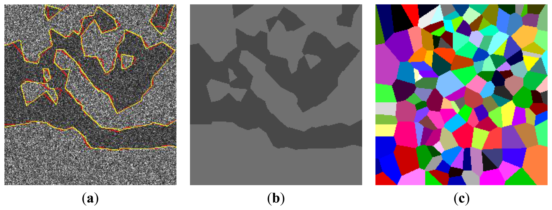
Figure 5 shows the final partitions with 152 polygons. Figure 5a, b gives the optimal segmentations obtained at 4,000 iterations, in which the segmented homogeneous regions are represented by their mean. To visually assess the accuracy for extracted dark spot regions, the extracted outlines of the segmented image in red and real outlines which is used for simulating image in yellow are both overlaid on the original images, see Figure 5c. Visually, the outlines of extracted oil spill regions(yellow) match their real outlines(red) very well.

In this experiment, two evaluation schemes are used to assess the accuracy of extracted oil spill area quantitatively. First of all, some of the common measures are used for accuracy assessment, including error matrix, producer's accuracy, consumer's accuracy, overall and Kappa coefficient.

Table 3. Error matrix and statistical measurements.

	C1	C2	ΣCs	Producer's Accuracy (%)
C1	39,908	1,448	41,356	94.13
C2.	971	23,209	24,180	97.61
ΣC.r	40,879	24,657	65,536	Overall accuracy (%)
User's accuracy (%)	95.98	96.95	0.92	96.3

gives the error matrixes which compare the segmented homogeneous regions as thematic classes to the real homogenous regions as reference.

The entries in the matrix contain a count of pixels, which is based on the labels assigned to pixels in both the segmented image and the synthesizing images. For example, if a pixel is segmented to the oil spill region with the label 1 and actually belongs to the water region with label 2, it will be counted in the error matrix entry of column 1 and row 2, denoted by C₁₂. The values of diagonal entries represent the count of correctly segmented pixels. The Table also lists row total (ΣC._r) and column total (ΣC_s.) which account for the total count of pixels segmented to regions r and belonging to regions s, respectively, where r, s ∈ {1, 2}. The value in the lower-right entry is the total number of pixels in the images.

Except for the error matrix, the associated accuracy estimates are used, including the producer's accuracy, consumer's accuracy, overall accuracy and Kappa coefficient. Table 3 also gives the values of those measures. In conclusion, one would anticipate a high degree of accuracy in the segmented results from the proposed algorithm. From Table 3, Kappa coefficients are calculated as 0.92. According to the general interpretation rules for thematic accuracy assessment, the Kappa coefficients 0.81–1.00 can be interpreted as almost perfect [25].

Another scheme for the accurate assessment of the developed segmentation algorithm is based on the degree to which the outlines of segmented homogeneous regions match their alternatives delineating the real regions, which is measured by the count of pixels of extracted outlines lying on the buffer zone around the real outlines of homogenous regions [9].

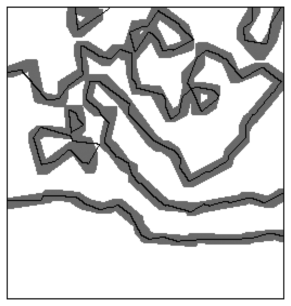
Figure 6 shows the extracted outlines of the extracted oil spill regions laid on the buffer zones with 4 pixels width around their real outlines at each side, in which the gray zones are buffer zones and the black lines are the outlines of segmented homogenous regions. It can be observed that almost all extracted outlines lay on the buffer zones.

Table 4. Percentage of extracted outlines in buffer zones.

B0(%)	B1/Σ1(%)	B2/Σ2(%)	B3/Σ3(%)	B4/Σ4(%)
35.7	39.6/75.3	15.6/90.9	5.7/96.6	1.7/98.3

gives the percents of the outlines for extracted oil spill regions on each buffer layer, where B₀ means the percent of the outlines exactly matching the outlines for the real oil spill regions in the synthesizing images. B_i's, here i = 1, 2, 3, 4, represent the percents of the extracted outlines of oil spill regions lying on the i'th buffer layer of the real outlines. The Table also gives the accumulated percents Σ_i = B₀ + B₁+ … + B_i. It can be seen from the Table that over 90% of the outlines of segmented homogenous regions are within the buffer zone with two pixel width around the outlines of real homogenous regions and almost all outlines (around 99%) of segmented homogenous regions are in the buffer zone with four pixel width around the outlines of real homogenous regions.

The results from above two accuracy analyses schemes manifest that the proposed algorithm extracts the shape and distribution parameters features of oil spill regions efficiently and effectively.

3.2. Real SAR Imagery

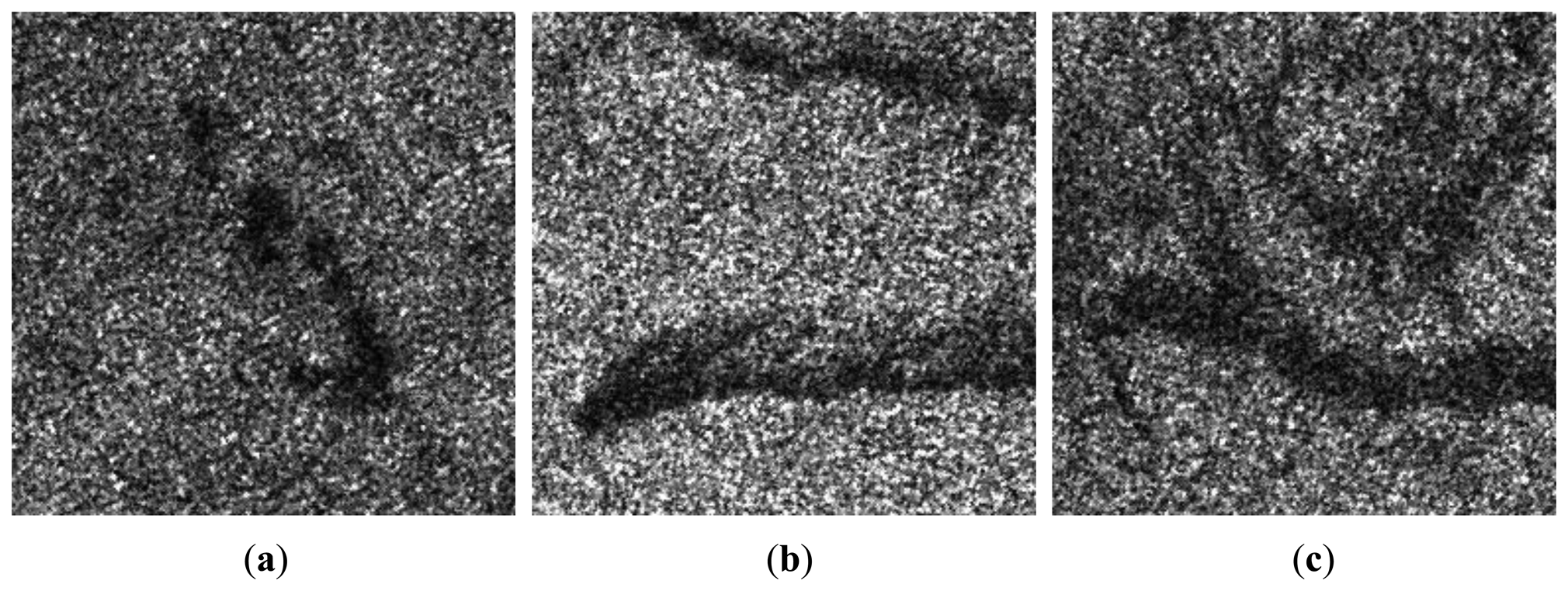
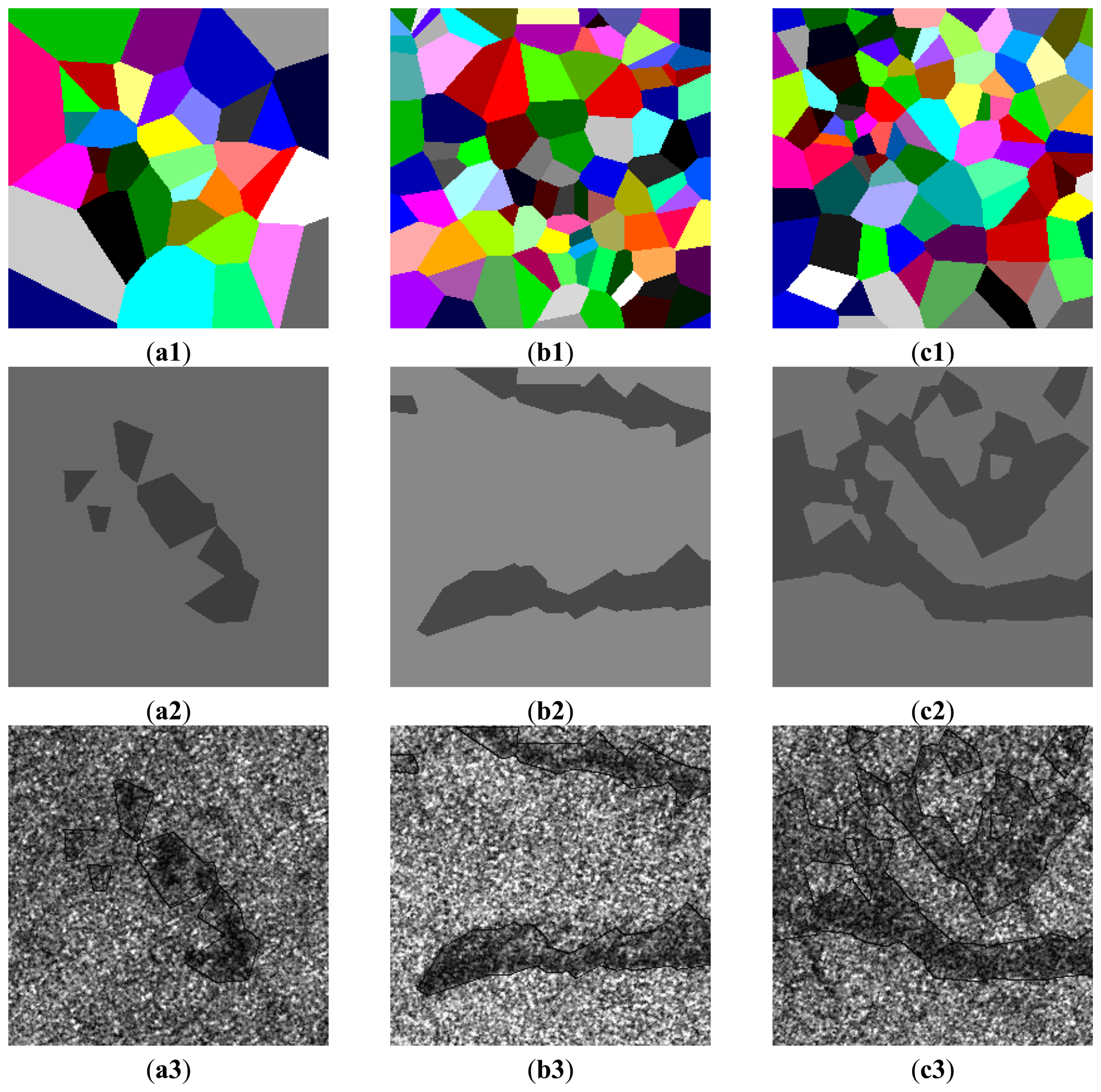
Figure 7 shows real SAR intensity images of RADARSAT-I/II HH polarization with oil slicks which appears darker compared to the surrounding waters. The initial partitions of image domain D are carried out by the Voronoi tessellation, in which the number of generating points m₀ is drawn from the Poisson distribution with the mean 96 and the locations of m₀ generating points are drawn from D uniformly. The initial segmentation is performed by randomly assigning a label to each polygon in the initial partition of D from the Bernoulli distribution with probabilities p_j = 1/2, where j = {1, …, m₀}. It is found that there is no obvious impact of the initial segmentation on the finial segmentation result. Figure 8a1, b1, c1 show the results of the final partitions of D with 36, 95 and 96 polygons, respectively. Figure 8a2, b2, c2 show the results of the optimal segmentation in terms of the MAP estimation after 4,000 iterations, where the tone for each region is represented by its estimated mean.

Figure 8a3, b3, c3 show the overlay of the outlines in black on the real SAR intensity images. Visually, the segmented regions match their real regions well.

Table 5. Estimated shape and scale parameters.

Image	α1	α2	β1	β2
a	5.00	3.22	28.27	23.11
b	4.06	2.44	28.64	34.02
c	4.72	2.67	31.02	32.44

summarizes estimated α_1,2 and β_1,2 corresponding to the segmented dark spot and sea regions.

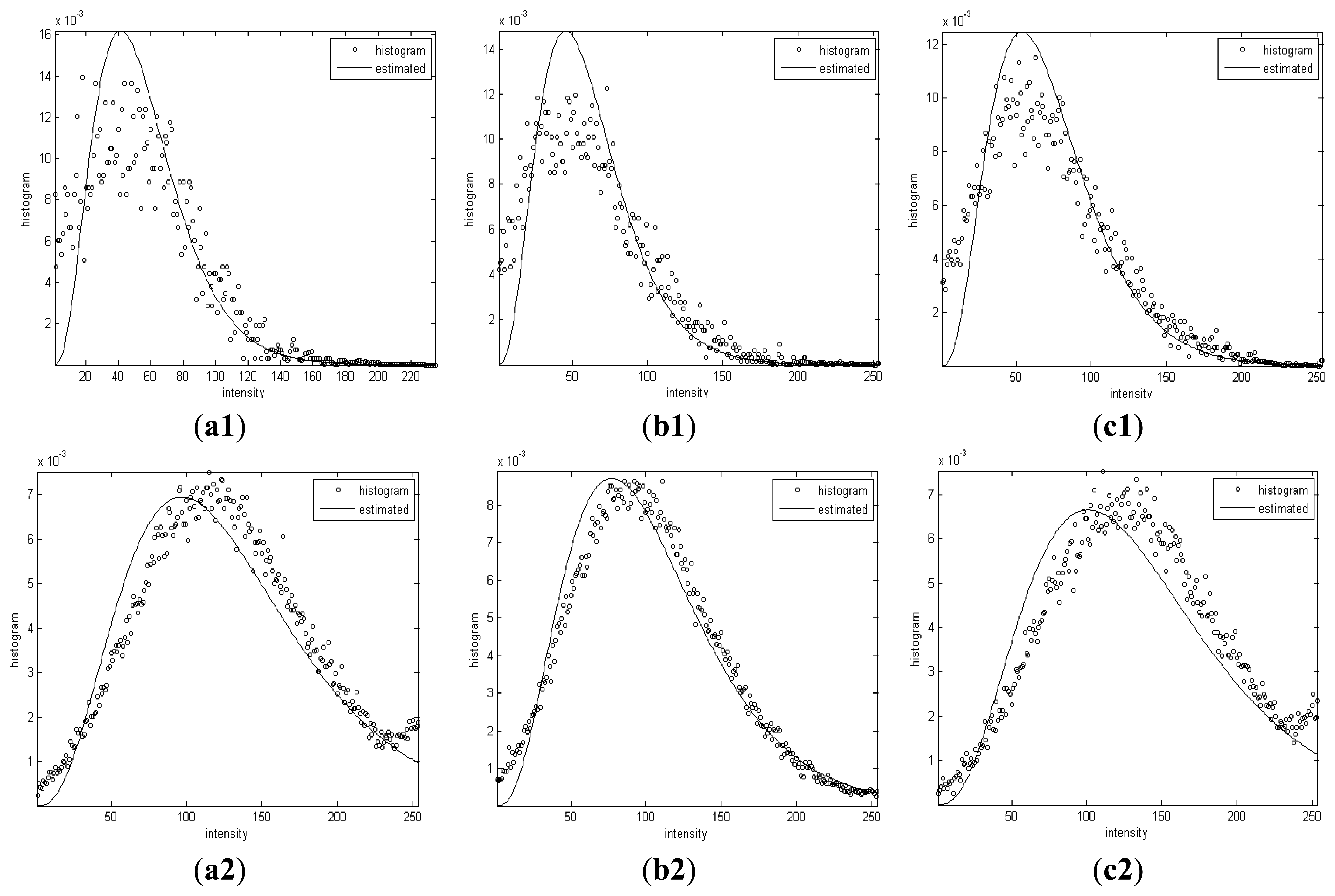
Figure 9 shows the histogram of intensities and Gamma distributions with the estimated shape and scale parameters of the segmented dark spots and sea background.

It can be observed that the histograms of intensities in each segmented homogenous region are coincident with the Gamma distribution curves with α and β derived by the proposed algorithm.

4. Conclusions

This paper presents a new segmentation-based approach to the feature extraction of oil spills from SAR intensity images, including their area and distribution parameters. The proposed segmentation algorithm is statistical region-based, which combines the Voronoi tessellation, Bayesian inference and reversible Jump Markov chain Monte Carlo (RJMCMC) methods. The Voronoi tessellation has been widely used to characterize models of many natural phenomena or processes in crystallography, metallography, physics, astrophysics, biology, ecology, geology, geography, etc.

In this paper the technique is introduced to design a region-based segmentation algorithm for oil spill feature extraction. By region, it means that Voronoi tessellation is used to partition the image domain into sub-regions (polygons) corresponding to components of oil spill regions or their surroundings (waters). Therefore, the segmentation of SAR intensity image for the purposes of oil spill feature extraction is completed by labeling those polygons as oil spills or water and thus modeled as a label field. By statistical, it means that each region (oil spill or water) is statistically homogenous, which is characterized by a Gamma distribution. Under the Bayesian inference paradigm, the label field for segmentation and distributing parameter can be expressed as a posterior conditional on a given SAR intensity image. The RJMCMC

method is employed to simulate the conditional posterior distribution. The results of testing the proposed approach on both real and synthesizing SAR intensity images demonstrate that it can extract the area and distribution parameters for oil spills with high accuracy and is promising.

References

- Mercier, G.; Girard-Ardhuin, F. Partially supervised oil-slick detection by SAR imagery using kernel expansion. IEEE Trans. Geosci. Remote Sens. 2006, 44, 2839–2846. [Google Scholar]
- Del Frate, F.; Petrocchi, A.; Lichtenegger, J.; Calabresi, G. Neural networks for oil spill detection using ERS-SAR data. IEEE Trans. Geosci. Remote Sens. 2000, 38, 2282–2287. [Google Scholar]
- Brekke, C.; Solberg, A.H.S. Classifiers and confidence estimation for oil spill detection in ENVISAT SAR Images. IEEE Geosci. Remote Sen. Lett. 2008, 5, 65–69. [Google Scholar]
- Topouzelis, K.; Karathanassi, V.; Pavlakis, P.; Rokos, D. Dark formation detection using neural networks. Int. J. Remote Sens. 2008, 29, 4705–4720. [Google Scholar]
- Bertacca, M.; Berizzi, F.; Mese, E. A FARIMA-based technique for oil slick and low-wind areas discrimination in sea SAR imagery. IEEE Trans. Geosci. Remote Sens. 2005, 43, 2484–2493. [Google Scholar]
- Brekke, C.; Solberg, A.H.S. Oil spill detection by satellite remote sensing. Remote Sens. Environ. 2005, 95, 1–13. [Google Scholar]
- Topouzelis, K.; Karathanassi, V.; Pavlakis, P.; Rokos, D. Detection and discrimination between oil spills and look-alike phenomena through neural networks. ISPRS J. Photogramm. Remote Sens. 2007, 62, 264–270. [Google Scholar]
- Topouzelis, K.; Psyllos, A. Oil spill feature selection and classification using decision tree forest on SAR image data. ISPRS J. Photogramm. Remote Sens. 2012, 68, 135–143. [Google Scholar]
- Li, Y.; Li, J. Oil spill detection from SAR intensity imagery using a marked point process. Remote Sens. Environ. 2010, 114, 1590–1601. [Google Scholar]
- Ferraro, G.; Baschek, B.; de Montpellier, G.; Njoten, O.; Perkovic, M.; Vespe, M. On the SAR derived alert in the detection of oil spills according to the analysis of the EGEMP. Mar. Poll. Bull. 2010, 60, 91–102. [Google Scholar]
- Bhogle, P.; Patil, S. Oil spill detection in SAR images using texture entropy algorithm and mahalanobis classifier. Int. J. Eng. Sci. 2012, 4, 4823–4826. [Google Scholar]
- Kanaa, T.; Tonye, E. Detection of Oil Slick Signatures in SAR Images by Fusion of Hysteresis Thresholding Responses. Proceedings of 2003 IEEE International Geoscience and Remote Sensing Symposium (IGARSS 2003), Toulouse, France, 21−25 July 2003; pp. 2750–2752.
- Mera, D.; Cotos, J.M.; Varela-Pet, J.; Garcia-Pineda, O. Adaptive thresholding algorithm based on SAR images and wind data to segment oil spills along the northwest coast of the Iberian Peninsula. Mar. Poll. Bull. 2012, 64, 2090–2096. [Google Scholar]
- Wu, S.Y.; Liu, A.K. Towards an automated ocean feature detection, extraction and classification scheme for SAR imagery. Int. J. Remote Sens. 2003, 24, 935–951. [Google Scholar]
- Barni, A.; Betti, M.; Mecocci, A. Fuzzy Segmentation of SAR Images for Oil Spill Recognition. Poceedings of Fifth International Conference on Image Processing and Its Applications, Edinburgh, UK, 4−6 July 1995; pp. 534–538.
- Lee, I.; Lee, K.; Torpelund-Bruin, C. Voronoi image segmentation and its applications to geoinformatics. J. Comput. 2009, 4, 1101–1108. [Google Scholar]
- Okabe, A.; Boots, B.; Sugihara, K.; Chiu, S. Spatial Tessellations: Concepts and Applications of Voronoi Diagrams; Barnett, V., Ed.; Wiley: Hoboken, NJ, USA, 2009; p. 671. [Google Scholar]
- Dryden, I.L.; Scarr, M.R.; Taylor, C.C. Bayesian texture segmentation of weed and crop images using reversible jump Markov chain Monte Carlo methods. J. R. Stat. Soc. 2003, 52, 31–50. [Google Scholar]
- Metropolis, N.; Rosenbluth, A. Equation of state calculations by fast computing machines. J. Chem. Phys. 1953, 21, 1087–1092. [Google Scholar]
- Hastings, W. Monte Carlo sampling methods using Markov chains and their applications. Biometrika 1970, 57, 97–109. [Google Scholar]
- Green, P.J. Reversible jump Markov chain Monte Carlo computation and bayesian model determination. Biometrika 1995, 82, 711–732. [Google Scholar]
- Green, P.; Sibson, R. Computing Dirichlet tessellations in the plane. Comput. J. 1978, 21, 168–173. [Google Scholar]
- Besag, J. Spatial interaction and the statistical analysis of lattice systems. J. R. Stat. Soc. B. 1974, 36, 192–236. [Google Scholar]
- Besag, J. On the statistical analysis of dirty pictures. J. R. Stat. Soc. B. 2008, 48, 259–302. [Google Scholar]
- Congalton, R.G.; Green, K. Assessing the Accuracy of Remotely Sensed Datasource, 2nd ed; CRC Press: New York, NY, USA, 2009; p. 183. [Google Scholar]