
A Model-Based Approach to Support Validation of Medical Cyber-Physical Systems


Abstract
:1. Introduction
- the models for clinical scenarios are restricted to the specific purpose of the system, without support to adapt the respective patient and device models for a new clinical context of interest, making its reuse unfeasible;
- the physical process simulation ignores important aspects of the clinical scenario dynamics, including external disturbances (e.g., user interventions) and particular reaction of each patient to the same stimuli (e.g., drug administration);
- the patient models either focus on variables of interest for specific clinical scenarios or neglect the relationship between the four human vital signs: heart and respiratory rates, blood pressure, and body temperature. The absence of this aspect contradicts the actual behavior of human beings [5,6]. Furthermore, when these models are formally defined in mathematical language they are not represented computationally and vice-versa. Therefore, these models have limited applicability to other scenarios.
2. Model Library: Building Reusable Models
2.1. Building Patient Models
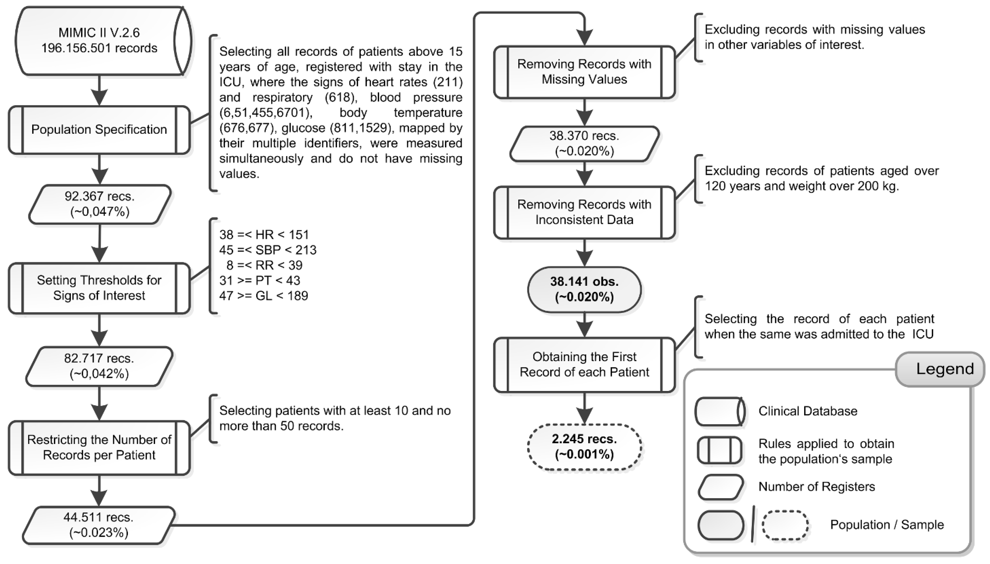
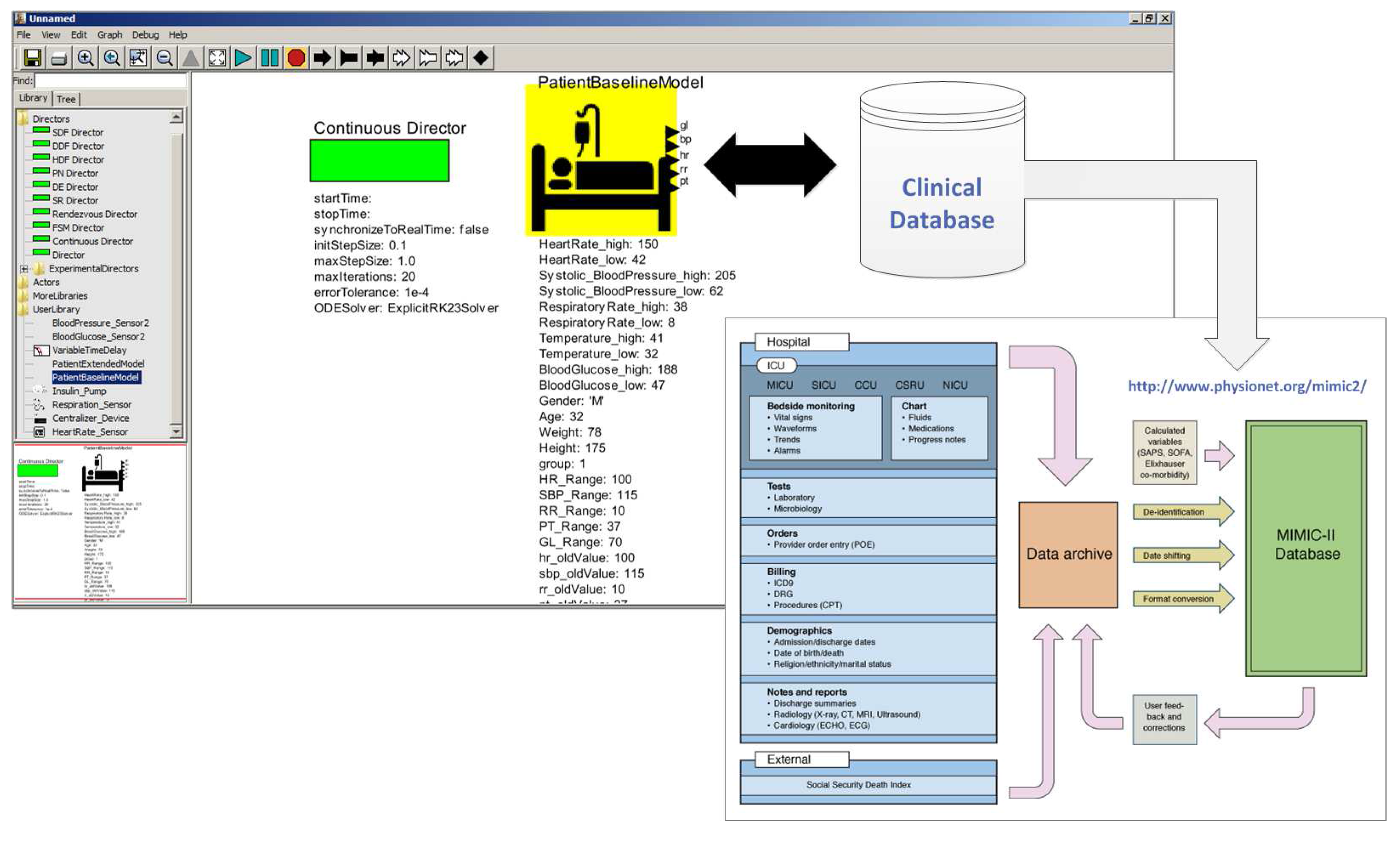
2.1.1. Stage 1—Choosing a Clinical Database


| Variable | Mean | Std. Dev. | CV | Minimum | Maximum |
|---|---|---|---|---|---|
| hr_value | 87.315 | 14.263 | 0.163 | 40.00 | 150.00 |
| sbp_value | 116.518 | 20.049 | 0.172 | 48.00 | 212.00 |
| rr_value | 19.216 | 5.628 | 0.293 | 8.00 | 38.00 |
| pt_value | 37.251 | 0.739 | 0.020 | 31.70 | 41.44 |
| gl_value | 118.761 | 27.802 | 0.234 | 47.00 | 188.00 |
| weight | 84.300 | 20.730 | 0.246 | 33.00 | 200.00 |
| height | 169.804 | 10.379 | 0.061 | 124.50 | 231.10 |
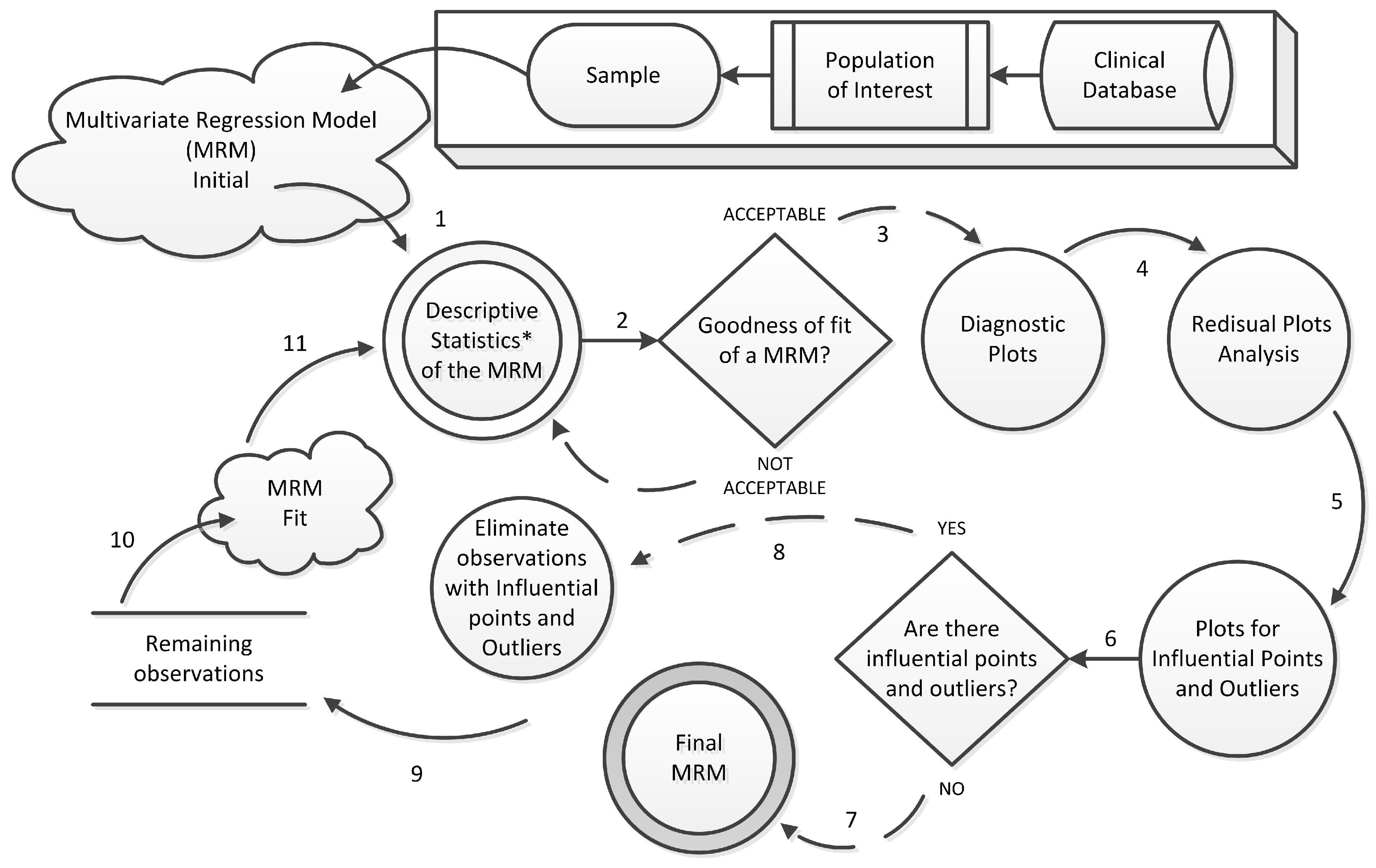
2.1.2. Stage 2—Obtaining a Statistical Model

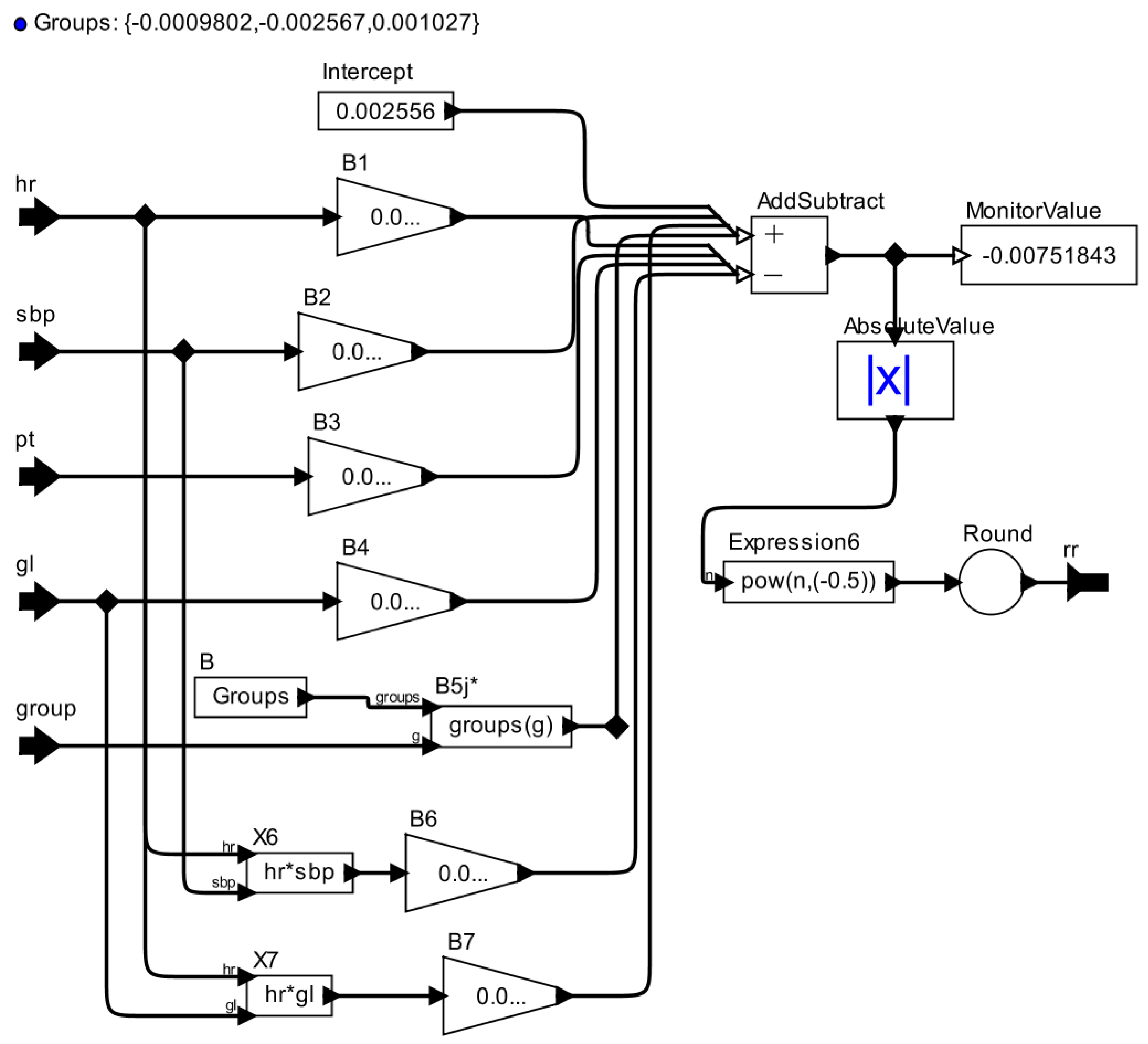
2.1.3. Stage 3—Developing an AOD Model
| Regression Model’s Term | AOD Actor | Actor’s Explanation |
|---|---|---|
| Intercept | Constant | Produce a constant output. The value of the output is that of the token contained by the value parameter, which by default is an integer with value 1. |
| Coefficient | Scale | Multiplies the input by a constant given as a parameter. |
| Predictor variable | Input port | An IOPort that defines the data type of an input. |
| Interaction between predictor variables | Expression | On each firing, evaluates an expression that may include references to the inputs, current time, and a count of the firing. The ports are referenced by the identifiers that have the same name as the port. |
| Math Symbols | AddSubtract | A polymorphic adder/subtractor. This adder has two input ports, both of which are multiports, and one output port, which is not. Data arriving on the input port named plus will be added, and data arriving on the input port named minus will be subtracted. |
| Expression | - | |
| Output port | An IOPort that defines the data type of an output. |


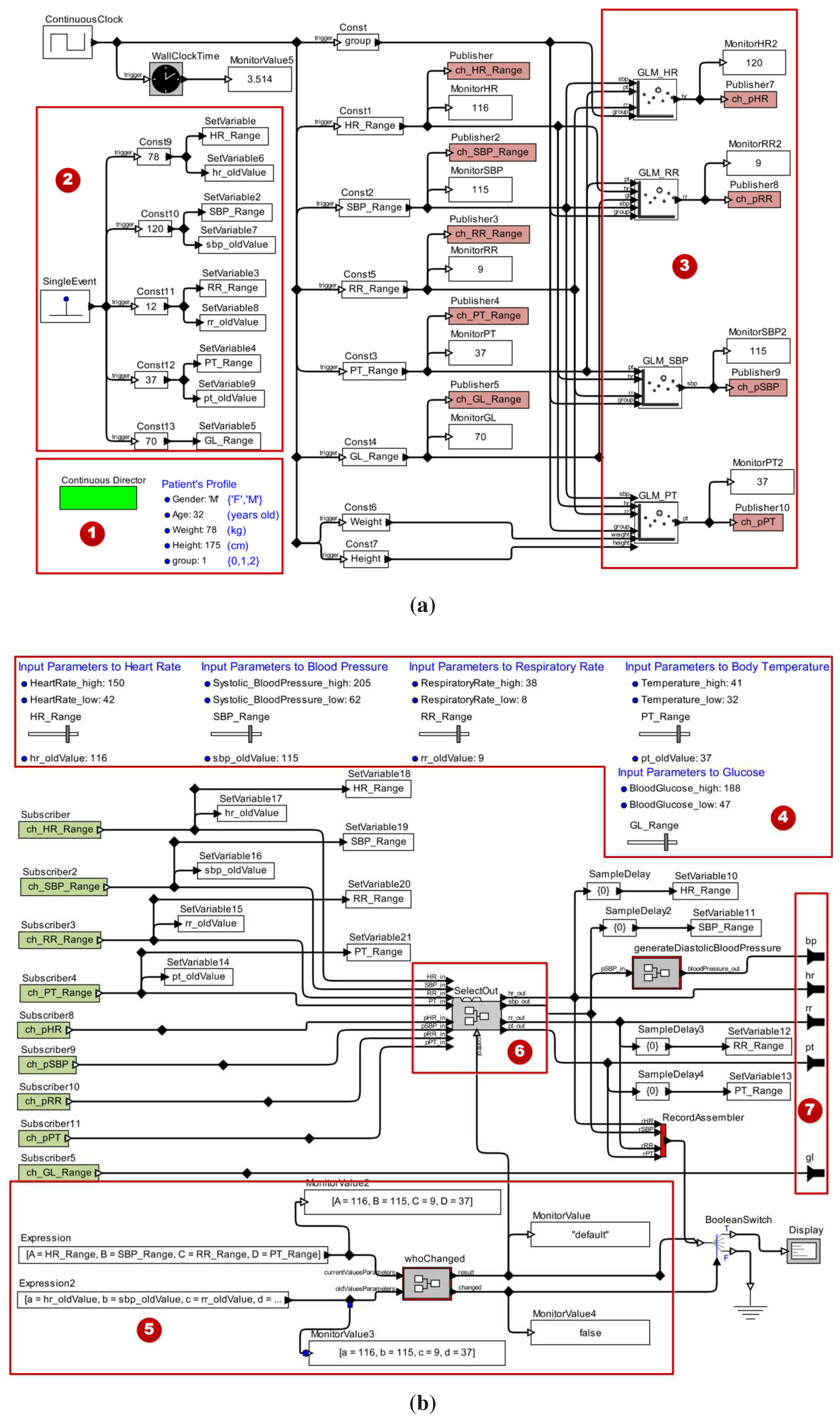
2.1.4. Stage 4—Validating the Patient Model

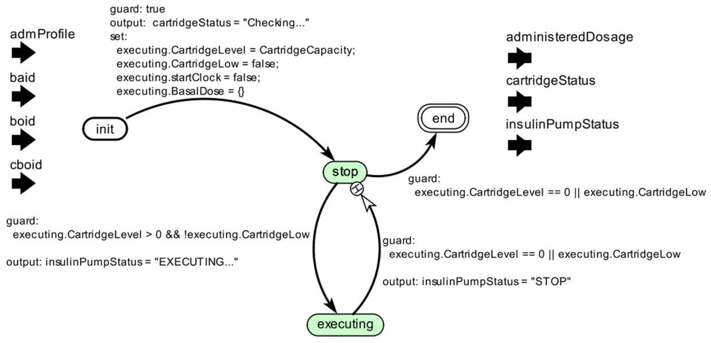
2.2. Building Medical Device Models
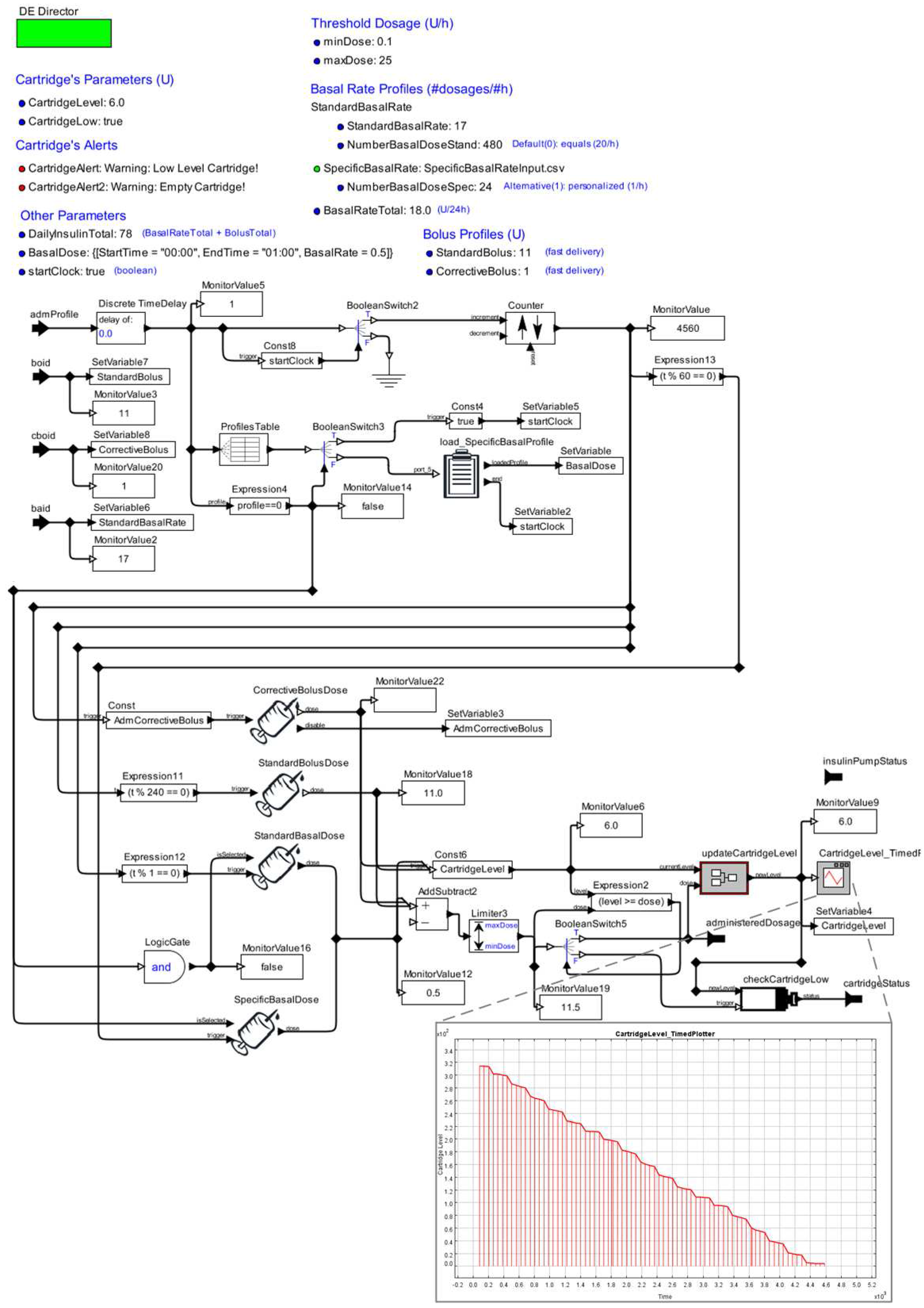
2.2.1. Stage 1—Choosing a Certified Medical Device
| Configuration Parameters | Functional Requirements | Safety Properties |
|---|---|---|
| 1. Insulin Type: U100 | 1. Operation Modes: Run/Stop; | 1. Errors (E) / Alerts (A): |
| 2. Cartridge Capacity: 3.15 mL | 2. Delivery Modes: Basal, Bolus and Corrective Bolus; | a. E: “Cartridge Empty!” |
| 3. Basal (U/h): | 3. Checking the cartridge level; | b. A: “Cartridge Low Warning!” |
| Min. = 0.1 | 4. Programming standard Bolus dose; | c. A: “Cartridge Ok!” |
| Max. = 25.0 | 5. Administrating corrective Bolus dose; | 2. State: |
| 4. Basal Profile: | 6. Providing information to the users. | a. “STOP” |
| a. Standard (# fixed dose/3min): 480 | b. “EXECUTING” | |
| b. Customized (# flexible dose/h): 24 | ||
| 5. Standard Bolus (U): Max. = 25.0 | ||
| 6. Administration Rate (dose/min): | ||
| a. Basal Dose | ||
| b. Bolus Dose |
2.2.2. Stage 2—Developing an AOD Model


2.2.3. Stage 3—Validating the Device Model
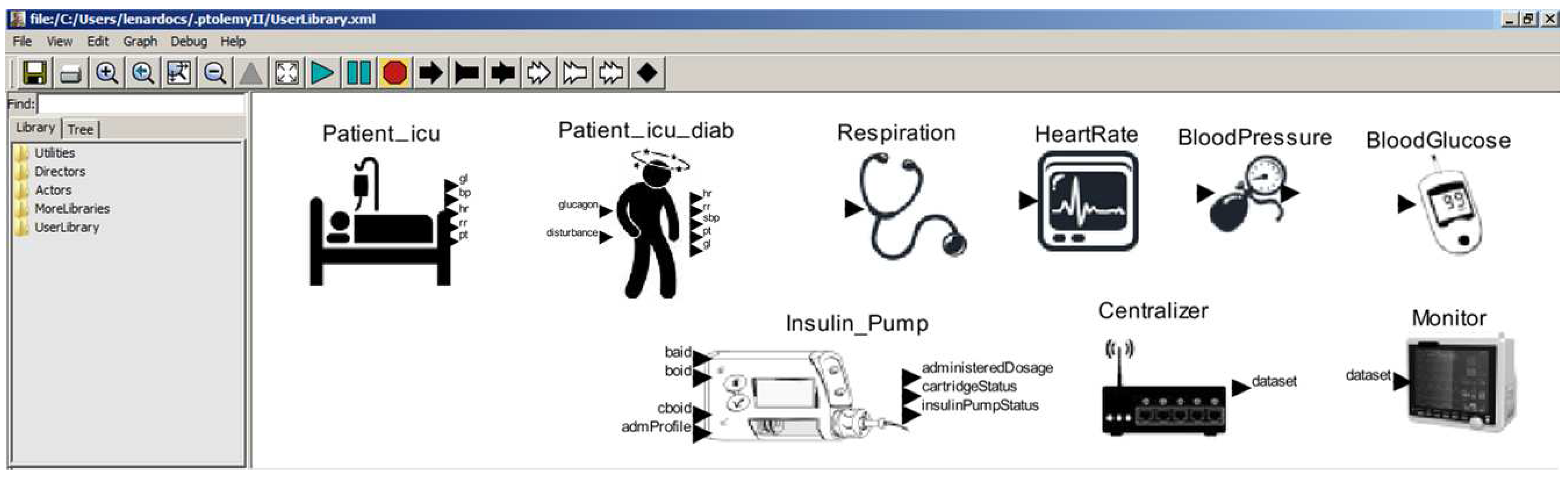
2.3. Model Library: Ready to be Reused


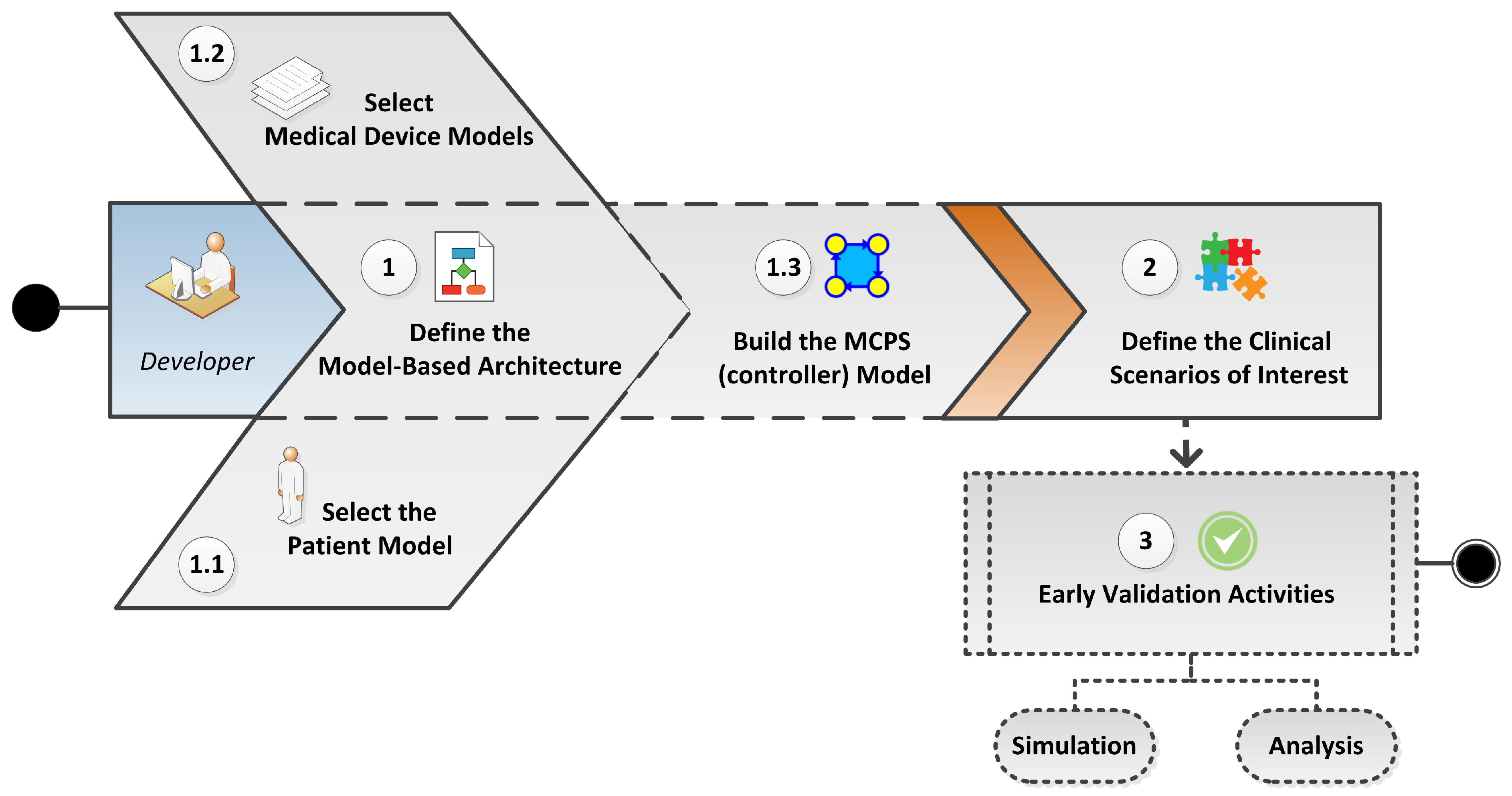
3. Composition and Simulation: Early Validation of MCPS


3.1. Designing the Model-Based Architecture
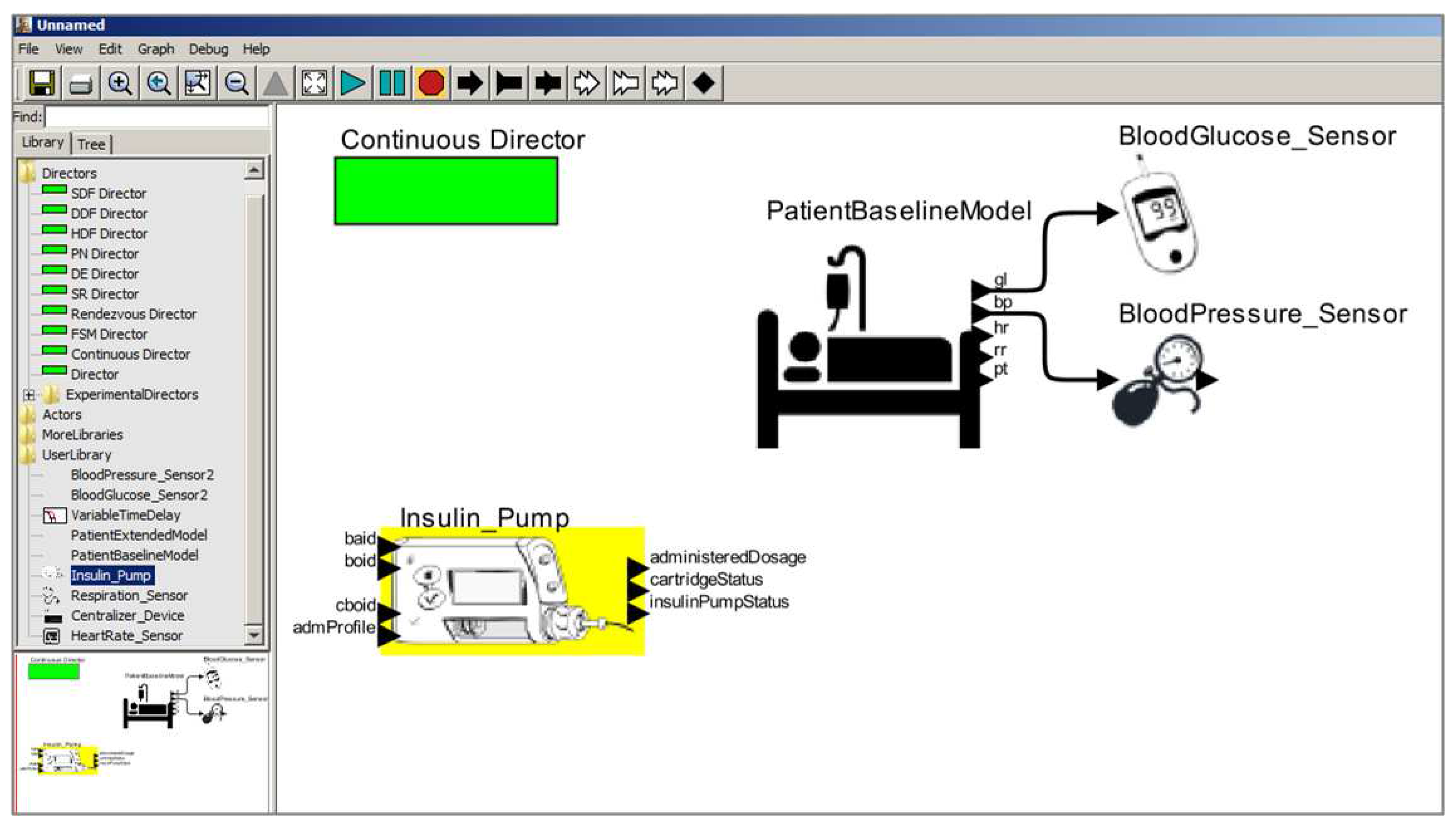
3.1.1. Selecting Patient Models

3.1.2. Selecting Medical Device Models

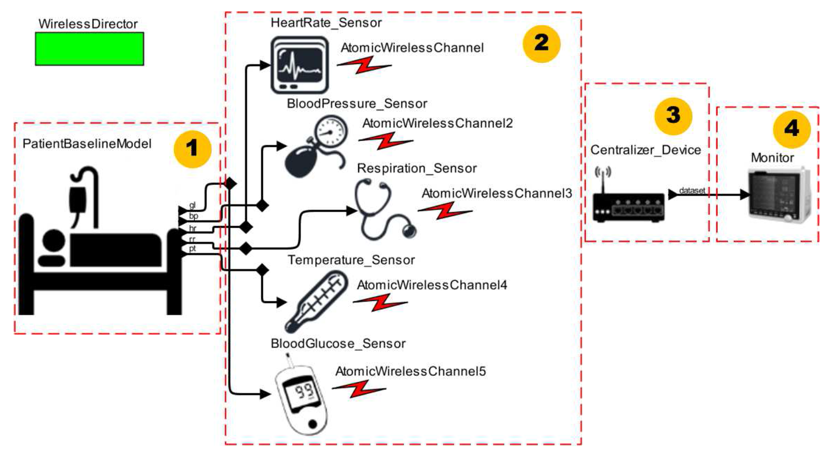
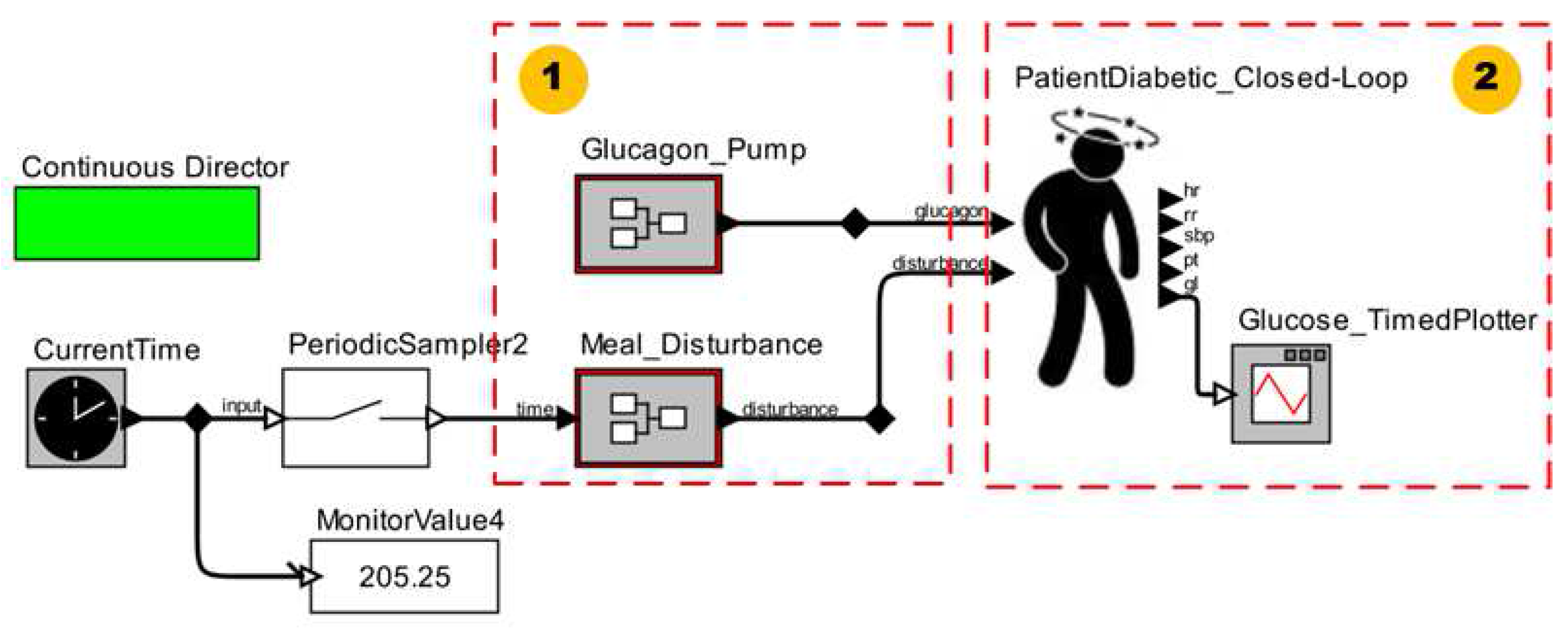
3.1.3. Composing the MCPS Model

3.2. Defining the Clinical Scenarios of Interest
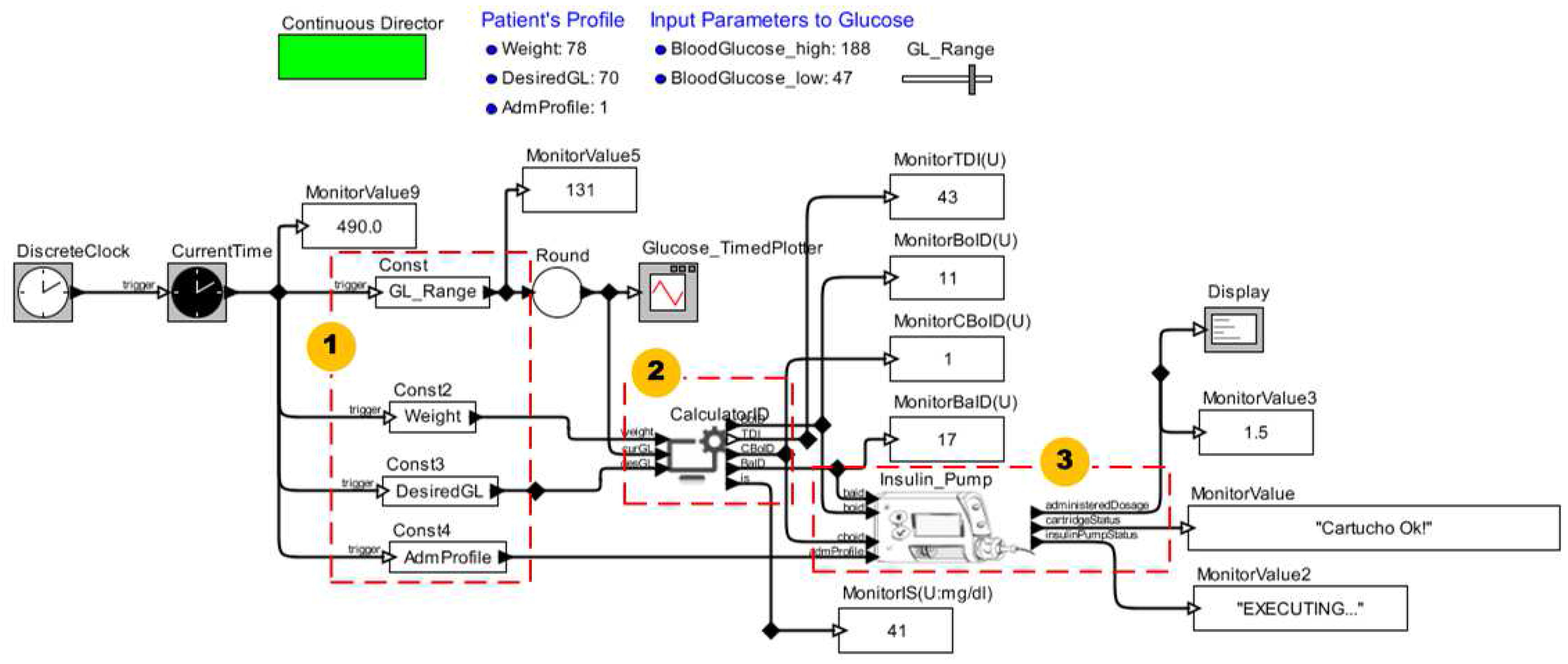
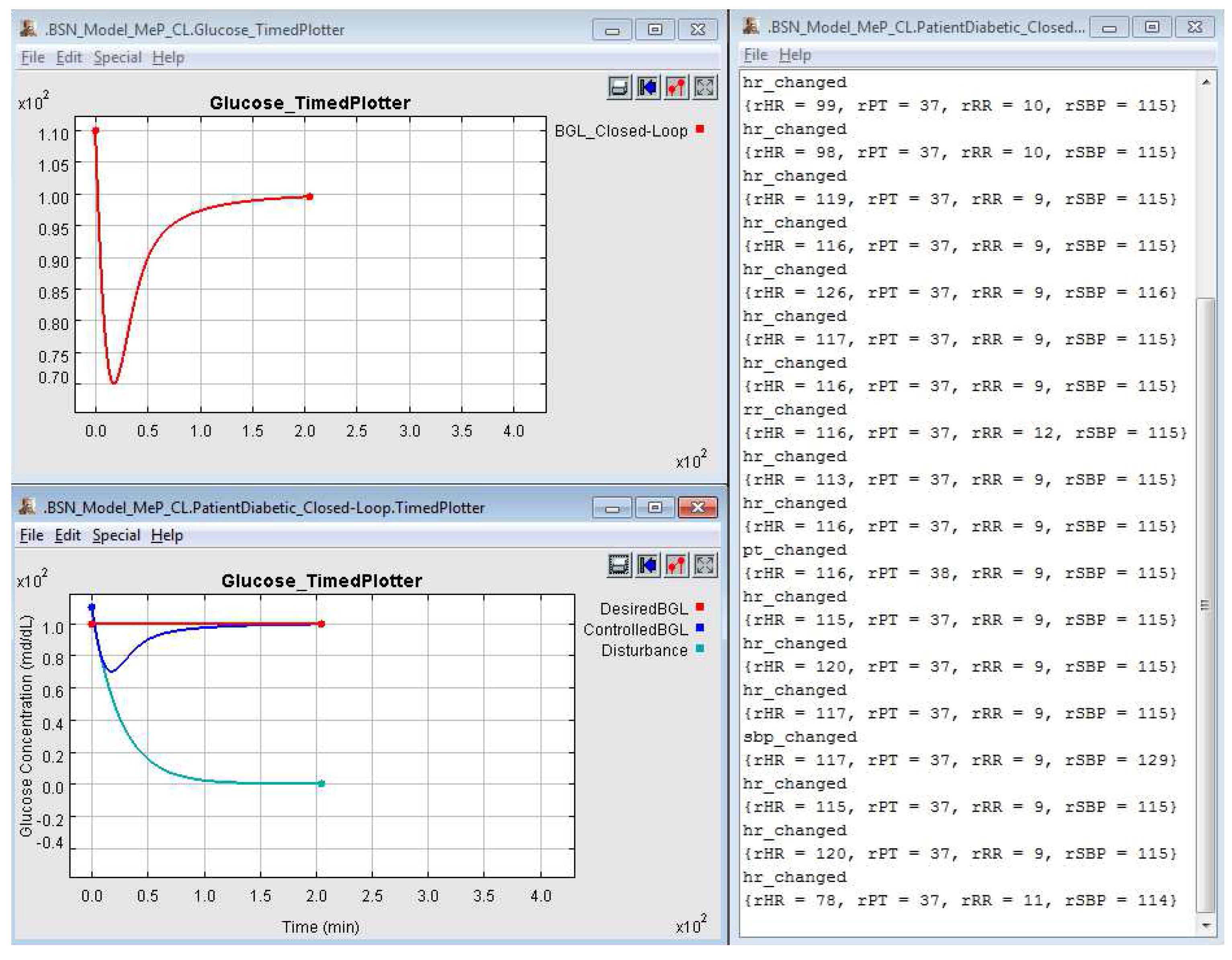
3.3. Running Early Validation Activities
4. Validation of the Proposed Approach
4.1. Validating the Approach for Different Clinical Scenarios
4.1.1. Clinical Context I


4.1.2. Clinical Context II

4.1.3. Clinical Context III


4.2. Empirical Evaluation
4.2.1. Scoping
- RQ1 Does using the library of patient and medical device models increase developers’ productivity?
- RQ2 Are the library’s models reusable?
- H0-1 Productivity is not increased.
- HA-1 Productivity is increased.
- H0-2 The models are not reusable.
- HA-2 The models are reusable.
4.2.2. Objects of study
4.2.3. Subjects
| Questions | Developers | |||||||||||||
|---|---|---|---|---|---|---|---|---|---|---|---|---|---|---|
| 1 | 2 | 3 | 4 | 5 | 6 | 7 | 8 | 9 | 10 | 11 | 12 | 13 | 14 | |
| Years Old | 21 | 25 | 20 | 21 | 30 | 21 | 24 | 27 | 21 | 21 | 20 | 25 | 22 | 23 |
| Knowledge on Formal Methods? | Y | Y | N | N | Y | Y | N | Y | N | Y | Y | Y | Y | Y |
| Opinion About the Training Phase? | GREAT | NORMAL | GOOD | GREAT | GOOD | GREAT | GREAT | GREAT | GREAT | GREAT | GOOD | GOOD | GOOD | GREAT |
| Resolved the list of exercises? | Y | Y | Y | Y | N | Y | Y | Y | Y | Y | Y | N | Y | N |
| Knowledge of Ptolemy II? | GOOD | GOOD | GOOD | NORMAL | LITTLE | GOOD | NORMAL | NORMAL | NORMAL | GOOD | NORMAL | NORMAL | GOOD | GOOD |
| Knowledge About Our Work? | GOOD | NORMAL | GOOD | NORMAL | LITTLE | GOOD | NORMAL | NORMAL | GOOD | GOOD | NORMAL | GOOD | GOOD | GOOD |
4.2.4. Variables and Treatment
4.2.5. Procedure
- Personal questionnaire—developers answer a questionnaire regarding personal information, experience with formal methods and experience with components reusability.
- Presentational learning—one of the researchers (i.e., trainer) gives an introductory course in which concepts regarding MCPS, Ptolemy II and the proposed method are presented. Furthermore, working examples of patient and device models in Ptolemy II are shown.
- Autonomous hands-on learning—(i.e., learning by doing) with online help from the trainer. The subjects applied the learned techniques to build simple elements in Ptolemy II such as an incremental counter and a sinusoidal signal sensor.
- MCPS modeling—the developers were divided into two balanced (i.e., same size) groups: control and treatment. Each group was composed of seven subjects selected randomly. The control group solved the two problems presented in Section 4.2.2 using only a small subset of the library of patient and medical device models. The treatment group solved the same problems using the entire library, except the centralizer device. Therefore, we used an experiment design of type “blocked subject-object study”. For the control group, we provided the heart and respiratory rate monitors, and glucometer completely ready for reuse, as well as the ICU patient and Insulin Pump models partially ready for reuse. Furthermore, for both groups, a guideline was provided to assist on the MCPS modeling.
- Reusability questionnaire reply—the developers responded to a questionnaire regarding the models’ reusability attributes: understandability, adaptability and portability.
4.2.6. Measures
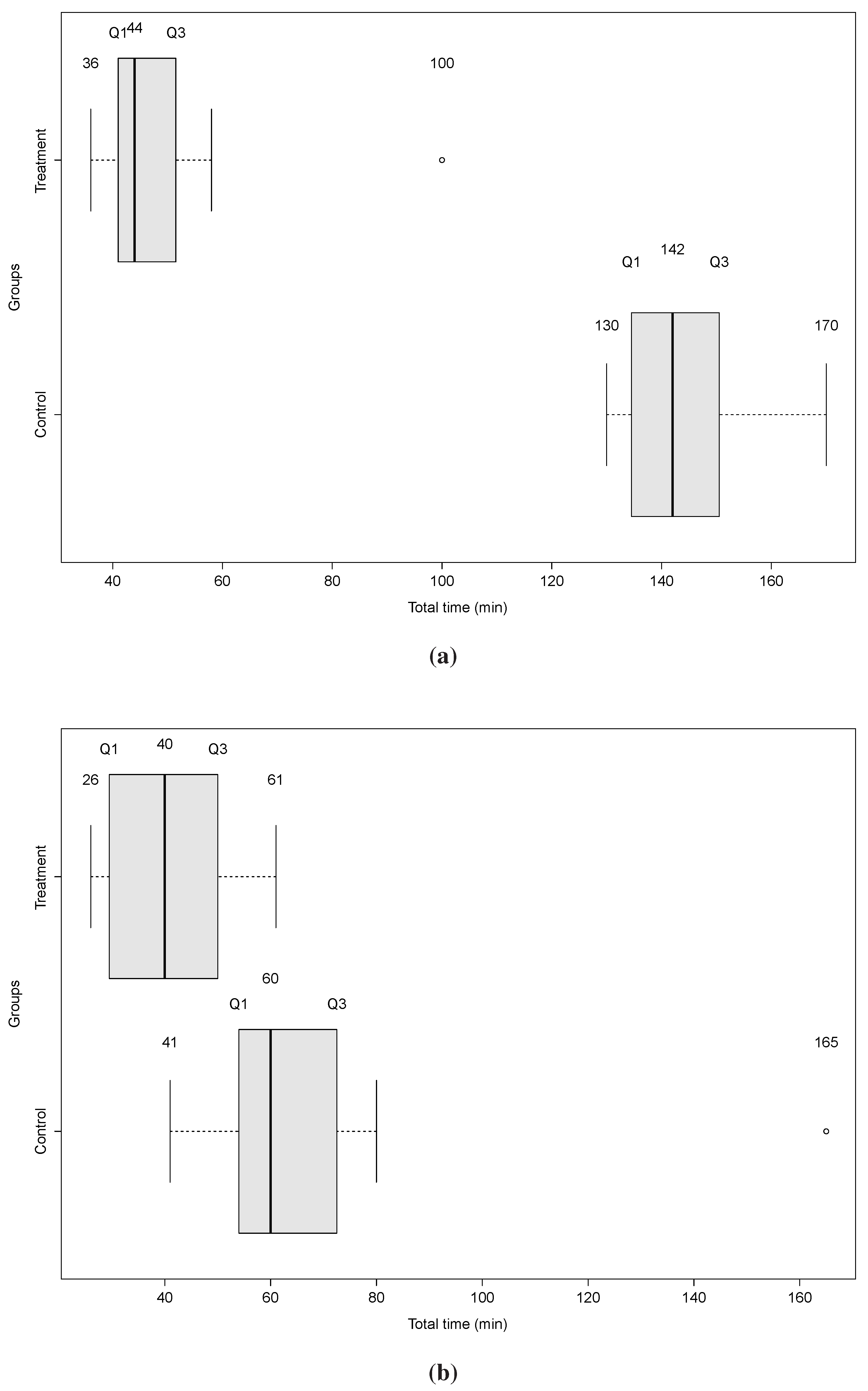
4.2.7. Analysis


4.2.8. Threats to Validity
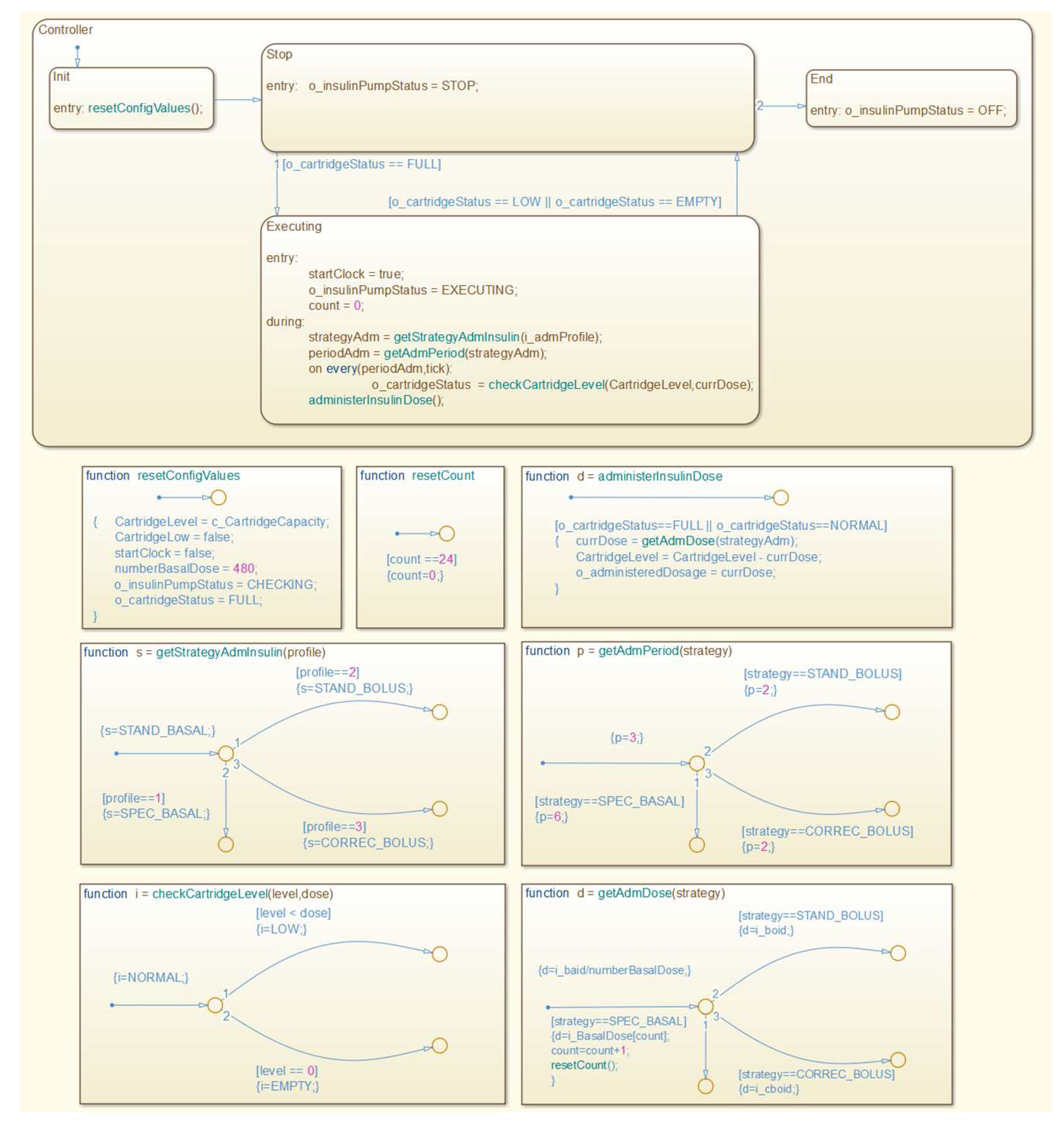
5. Model Analysis
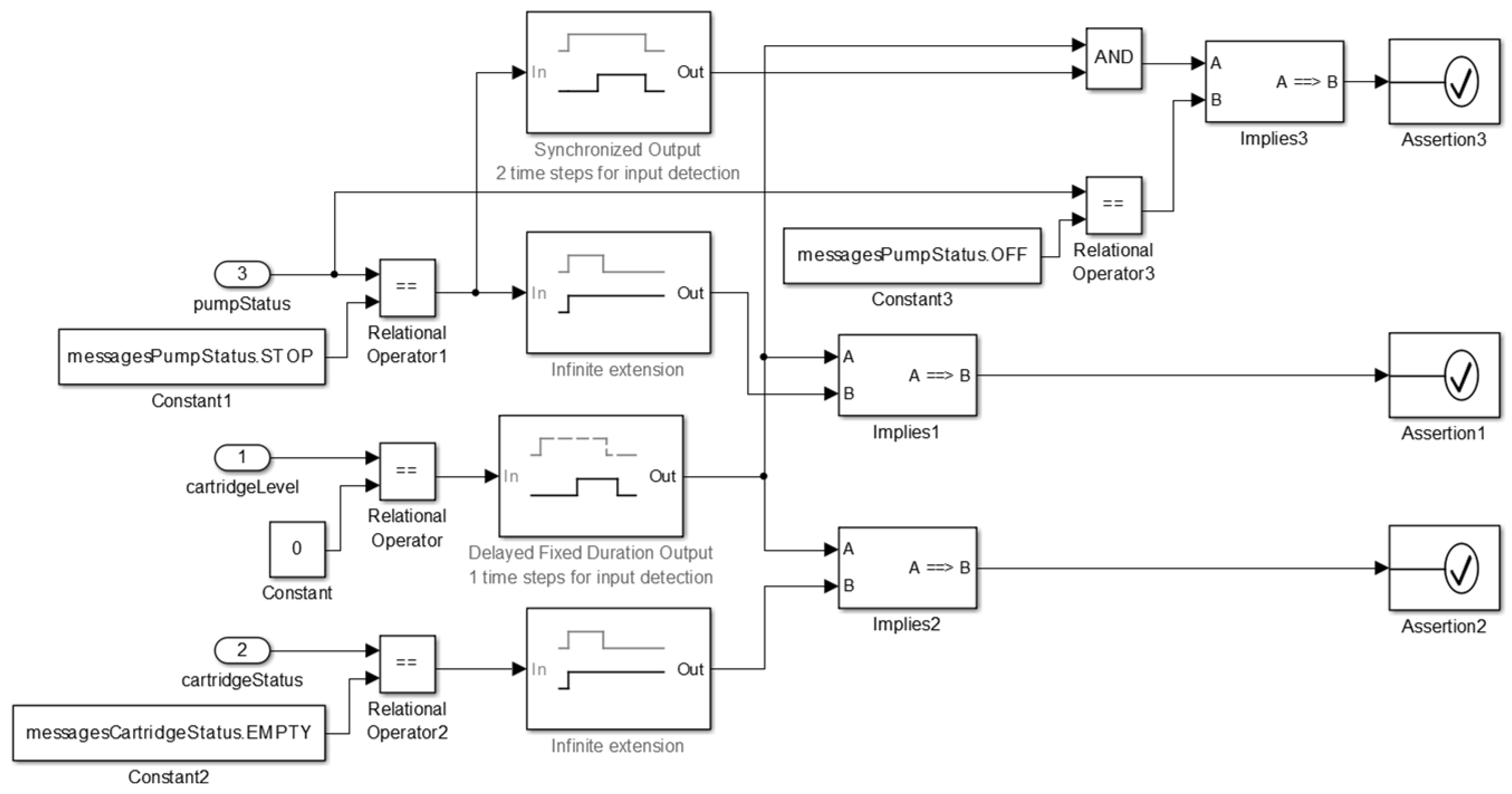
- Safety Requirement 1 (SR1):
- if cartridge’s level is equal to 0, then the cartridge’s status shall become EMPTY and after a delay the pump’s status shall be STOP. The formalization of this property is shown in Figure 26.
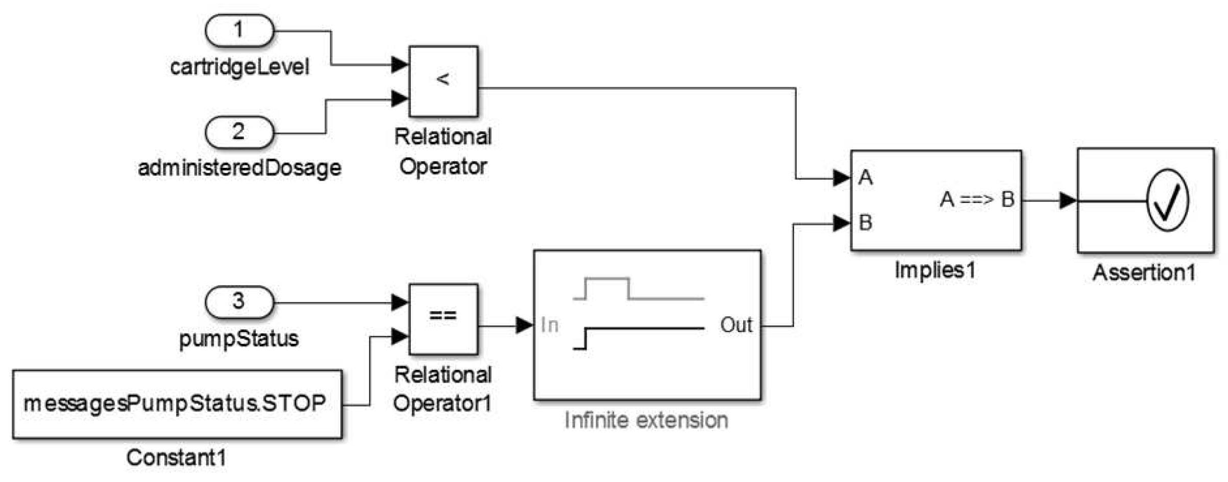
- Safety Requirement 2 (SR2):
- if cartridge’s level is lower than the administered insulin dosage then the pump’s status shall be STOP. The formalization of this property is shown in Figure 27.
- Safety Requirement 3 (SR3):
- whenever the administration profile becomes 1 (SPEC_BASAL) the administered dosage shall equal the programmed dosage. The formalization of this property is shown in Figure 28.


| Model Hierarchy | Cyclomatic Complexity | DC | CC | MDCC |
|---|---|---|---|---|
| Subsystem:Insulin Pump Software Model | 22 | 92% | 75% | 50% |
| Chart:Insulin Pump Software Model | 21 | 92% | 75% | 50% |
| State:Controller | 7 | 100% | 75% | 50% |
| Function:administerInsulinDose | 2 | 100% | 75% | 50% |
| Function:checkCartridgeLevel | 2 | 75% | NA | NA |
| Function:getAdmDose | 3 | 67% | NA | NA |
| Function:getAdmPeriod | 3 | 100% | NA | NA |
| Function:getStrategyAdmInsulin | 3 | 100% | NA | NA |
| Function:resetCount | 1 | 100% | NA | NA |
6. Conclusions
Acknowledgments
Author Contributions
Conflicts of Interest
References
- Arney, D.; Plourde, J.; Schrenker, R.; Mattegunta, P.; Whitehead, S.F.; Goldman, J.M. Design Pillars for Medical Cyber-Physical System Middleware. OpenAccess Ser. Inform. 2014, 36, 124–132. [Google Scholar]
- Haque, S.A.; Aziz, S.M.; Rahman, M. Review of Cyber-Physical System in Healthcare. Int. J. Distrib. Sens. Netw. 2014. [Google Scholar] [CrossRef]
- Lee, I.; Sokolsky, O.; Chen, S.; Hatcliff, J.; Jee, E.; Kim, B.; King, A.; Mullen-Fortino, M.; Park, S.; Roederer, A.; et al. Challenges and research directions in medical cyber-physical systems. IEEE Proc. 2012, 100, 75–90. [Google Scholar] [CrossRef]
- Lee, E. The Past, Present and Future of Cyber-Physical Systems: A Focus on Models. Sensors 2015, 15, 4837–4869. [Google Scholar] [CrossRef] [PubMed]
- Delaune, S.C.; Ladner, P.K. Fundamentals of Nursing: Standards & Practice, 4th ed.; Cengage Learning: Clifton Park, NY, USA, 2011. [Google Scholar]
- Rosdahl, C.B.; Kowalski, M.T. Textbook of Basic Nursing, 10th ed.; Wolters Kluwer Health Lippincott Williams & Wilkins: Philadelphia, PA, USA, 2012. [Google Scholar]
- González, J.V.; Arenas, O.A.V.; González, V.V. Semiología de los Signos Vitales: Una Mirada Novedosa a un Problema Vigente. Arch. Med. 2012, 12, 221–240. [Google Scholar]
- FDA. CFR—Code of Federal Regulations Title 21—Part 820. Available online: http://www.accessdata.fda.gov/scripts/cdrh/cfdocs/cfcfr/CFRSearch.cfm?CFRPart=820 (accessed on 11 September 2014).
- Li, T.; Tan, F.; Wang, Q.; Bu, L.; Cao, J.-N.; Liu, X. From Offline toward Real Time: A Hybrid Systems Model Checking and CPS Codesign Approach for Medical Device Plug-and-Play Collaborations. IEEE Trans. Parallel Distrib. Syst. 2014, 25, 642–652. [Google Scholar] [CrossRef]
- Hassine, J. Early modeling and validation of timed system requirements using Timed Use Case Maps. Requir. Eng. 2015, 20, 181–211. [Google Scholar] [CrossRef]
- FDA. Medical Device Recall Report—FY2003 to FY2012; Technical Report; U.S. Food and Drug Administration (FDA)—Department of Health and Human Services, Center for Devices and Radiological Health (CDRH). Available online: http://www.webcitation.org/6ZdUQoc4Q (accessed on 11 September 2014).
- ASTM International. ASTM F2761-09(2013). Medical Devices and Medical Systems Essential Safety Requirements for Equipment Comprising the Patient-Centric Integrated Clinical Environment (ICE), Part 1: General Requirements and Conceptual Model. Available online: http://www.webcitation.org/6ZdV3vBC1 (accessed on 23 March 2013).
- Pajic, M.; Mangharam, R.; Sokolsky, O.; Arney, D.; Goldman, J.; Lee, I. Model-Driven Safety Analysis of Closed-Loop Medical Systems. IEEE Trans. Ind. Inform. 2012, 10, 3–16. [Google Scholar] [CrossRef] [PubMed]
- Jiang, Z.; Pajic, M.; Mangharam, R. Cyber-Physical Modeling of Implantable Cardiac Medical Devices. IEEE Proc. 2012, 100, 122–137. [Google Scholar] [CrossRef]
- Jiang, Z.; Pajic, M.; Alur, R.; Mangharam, R. Closed-loop verification of medical devices with model abstraction and refinement. Int. J. Softw. Tools Technol. Transf. 2014, 16, 191–213. [Google Scholar] [CrossRef]
- Miller, B.; Vahid, F.; Givargis, T. Digital Mockups for the Testing of a Medical Ventilator. In Proceedings of the 2nd ACM SIGHIT International Health Informatics Symposium (IHI), Miami, FL, USA, 28–30 January 2012; pp. 859–862.
- Van Heusden, K.; Dassau, E.; Zisser, H.C.; Seborg, D.E.; Doyle, F.J. Control-Relevant Models for Glucose Control Using A Priori Patient Characteristics. IEEE Trans. Biomed. Eng. 2012, 59, 1839–1849. [Google Scholar] [CrossRef] [PubMed]
- Kang, W.; Wu, P.; Rahmaniheris, M.; Sha, L.; Berlin, R.B.; Goldman, J.M. Towards organ-centric compositional development of safe networked supervisory medical systems. In Proceedings of the IEEE 26th International Symposium on Computer-Based Medical Systems (CBMS), Porto, Portugal, 20–22 June 2013; pp. 143–148.
- King, A.L.; Feng, L.; Sokolsky, O.; Lee, I. Assuring the safety of on-demand medical cyber-physical systems. In Proceedings of the IEEE 1st International Conference on Cyber-Physical Systems, Networks, and Applications (CPSNA), Taipei, Taiwan, 19–20 August 2013; pp. 1–6.
- Simalatsar, A.; de Micheli, G. Medical guidelines reconciling medical software and electronic devices: Imatinib case-study. In Proceedings of the IEEE 12th International Conference on Bioinformatics Bioengineering (BIBE), Larnaca, Cyprus, 11–13 November 2012; pp. 19–24.
- Li, C.; Raghunathan, A.; Jha, N.K. Improving the Trustworthiness of Medical Device Software with Formal Verification Methods. IEEE Embed. Syst. Lett. 2013, 5, 50–53. [Google Scholar] [CrossRef]
- Murugesan, A.; Sokolsky, O.; Rayadurgam, S.; Whalen, M.; Heimdahl, M.; Lee, I. Linking abstract analysis to concrete design: A hierarchical approach to verify medical CPS safety. In Proceedings of the ACM/IEEE 5th International Conference on Cyber-Physical Systems (ICCPS), Berlin, Germany, 14–17 April 2014; pp. 139–150.
- Agha, G. Actors: A Model of Concurrent Computation in Distributed Systems; MIT Press: Cambridge, MA, USA, 1986. [Google Scholar]
- Basili, V.R.; Rombach, H.D. The TAME project: Towards improvement-oriented software environments. IEEE Trans. Softw. Eng. 1988, 14, 758–773. [Google Scholar] [CrossRef]
- Mathworks. Simulink Design Verifier. 2012. Available online: http://www.mathworks.com/products/sldesignverifier (accessed on 30 July 2015).
- Berkeley, U.C. The Ptolemy Project: Heterogeneous, Modeling and Design; EECS Dept. Available online: http://ptolemy.eecs.berkeley.edu/ptolemyII (accessed on 12 September 2012).
- Katzung, B.G. Introduction. In Basic & Clinical Pharmacology, 12th ed.; Katzung, B.G., Masters, S.B., Trevor, A.J., Eds.; McGraw-Hill Companies, Inc.: West Windsor Township, NJ, USA, 2012. [Google Scholar]
- Hair, J.F.; Black, W.C.; Babin, B.J.; Anderson, R.E.; Tatham, R.L. Análise Multivariada de Dados, 6th ed.; Bookman: Porto Alegre, Brazil, 2009. [Google Scholar]
- PHYSIONET. MIMIC II Databases, National Institutes of Health (NIH), 2009. Available online: http://physionet.org/mimic2 (accessed on 13 September 2013).
- ADA. Diagnosis and Classification of Diabetes Mellitus. Diabetes Care 2004, 27, s5–s10. [Google Scholar] [CrossRef] [PubMed]
- Buxton, A.E.; Calkins, H.; Callans, D.J.; DiMarco, J.P.; Fisher, J.D.; Greene, H.L.; Haines, D.E.; Hayes, D.L.; Heidenreich, P.A.; Miller, J.M.; et al. ACC/AHA/HRS 2006 Key Data Elements and Definitions for Electrophysiological Studies and Procedures: A Report of the American College of Cardiology/American Heart Association Task Force on Clinical Data Standards (ACC/AHA/HRS Writing Committee to Develop Data Standards on Electrophysiology). J. Am. Coll. Cardiol. 2006, 48, 2360–2396. [Google Scholar] [PubMed]
- Chobanian, A.V.; Bakris, G.L.; Black, H.R.; Cushman, W.C.; Green, L.A.; Izzo, J.L., Jr.; Jones, D.W.; Materson, B.J.; Oparil, S.; Wright, J.T., Jr.; et al. Seventh Report of the Joint National Committee on Prevention, Detection, Evaluation, and Treatment of High Blood Pressure. Hypertension 2003, 42, 1206–1252. [Google Scholar] [CrossRef] [PubMed]
- Handelsman, Y.; Mechanick, J.; Blonde, L.; Grunberger, G.; Bloomgarden, Z.T.; Bray, G.A.; Dagogo-Jack, S.; Davidson, J.A.; Einhorn, D.; Ganda, O.; et al. American Association of Clinical Endocrinologists Medical Guidelines for Clinical Practice for Developing a Diabetes Mellitus Comprehensive Care Plan: Executive Summary. Endocr. Pract. 2011, 17, 287–302. [Google Scholar] [CrossRef] [PubMed]
- McGee, S.R. Evidence-Based Physical Diagnosis, 2nd ed.; Saunders Elsevier: St. Louis, MO, USA, 2007. [Google Scholar]
- NHBPEP. The Fourth Report on the Diagnosis, Evaluation, and Treatment of High Blood Pressure in Children and Adolescents. Pediatrics 2004, 114 (Suppl. 2), 555–576. [Google Scholar] [CrossRef] [PubMed]
- Jain, R. The Art of Computer Systems Performance Analysis: Techniques for Experimental Design, Measurement, Simulation, and Modeling; John Wiley & Sons, Inc.: New York, NY, USA, 1991. [Google Scholar]
- McCullagh, P.; Nelder, J.A. Generalized Linear Models, 2nd ed.; Chapman and Hall: London, UK, 1989. [Google Scholar]
- Cassandras, C.G.; Lafortune, S. Introduction to Discrete Event Systems, 2nd ed.; Springer: New York, NY, USA, 2008. [Google Scholar]
- Mathworks. PID Controller, Discrete PID Controller. Available online: http://www.mathworks.com/help/simulink/slref/pidcontroller.html (accessed on 22 May 2014).
- Mathworks. MATLAB. Available online: http://www.mathworks.com/products/matlab/ (accessed on 10 June 2015).
- Bergman, R.N.; Phillips, L.S.; Cobelli, C. Physiologic Evaluation of Factors Controlling Glucose Tolerance in Man: Measurement of Insulin Sensitivity and Beta-Cell Glucose Sensitivity from the Response to Intravenous Glucose. J. Clin. Investig. 1981, 68, 1456–1467. [Google Scholar] [CrossRef] [PubMed]
- Khan, S.H.; Khan, A.H.; Khan, Z.H. Artificial Pancreas Coupled Vital Signs Monitoring for Improved Patient Safety. Arab. J. Sci. Eng. 2013, 38, 3093–3102. [Google Scholar] [CrossRef]
- Franklin, G.F.; Powell, J.D.; Emami-Naeini, A. Feedback Control of Dynamic Systems, 4th ed.; Prentice Hall: Upper Saddle River, NJ, USA, 2002. [Google Scholar]
- Ogata, K. Modern Control Engineering, 3rd ed.; Prentice Hall: Hackensack, NJ, USA, 1997. [Google Scholar]
- FDA. Classify Your Medical Device. Available online: http://www.webcitation.org/6ZdUv0YwI (accessed on 11 September 2014).
- ROCHE. ACCU-CHEK Spirit Insulin Pump System: Pump User Guide. Roche Health Solutions Inc., 2008. Available online: http://www.webcitation.org/6ZdVHOgBx (accessed on 20 May 2013).
- Diabetes.co.uk. Basal Bolus—Basal Bolus Injection Regimen. Available online: http://www.webcitation.org/6ZdVLD7NE (accessed on 5 March 2014).
- Lee, E.A.; Seshia, S.A. Introduction to Embedded Systems, A Cyber-Physical Systems Approach, 2nd ed.; LeeSeshia.Org.: Philadelphia, PA, USA, 2015. [Google Scholar]
- Silva, L.C.; Perkusich, M.; Bublitz, F.M.; Almeida, H.O.; Perkusich, A. A Model-Based Architecture for Testing Medical Cyber-Physical Systems. In Proceedings of the 29th Annual ACM Symposium on Applied Computing (SAC), Gyeongju, Korea, 24–28 March 2014; pp. 25–30.
- Ptolemaeus, C. System Design, Modeling, and Simulation Using Ptolemy II; Ptolemy.Org: Berkeley, CA, USA, 2014. [Google Scholar]
- Silva, L.C.; Almeida, H.O.; Perkusich, A.; Perkusich, M. A Model-Based Approach to Support Validation of Medical Cyber-Physical Systems. Supplementary Material. 2015. Available online: http://sites.google.com/site/mbatomcps/ (accessed on 28 October 2015).
- NIH. Asthma. National Institutes of Health, 2014. Available online: http://www.nhlbi.nih.gov/health/health-topics/topics/asthma (accessed on 17 August 2014). [Google Scholar]
- WHO. 10 Facts about Diabetes. World Health Organization, 2013. Available online: http://www.webcitation.org/6ZdVT2Scz (accessed on 29 November 2014).
- WHO. World Health Statistics. Global Health Observatory (GHO), World Health Organization, 2012. Available online: http://www.who.int/gho/publications/world_health_statistics/2012/en/ (accessed on 15 March 2014).
- Gomes, M.B.; Lerario, A.C. Gerenciamento Eletrônico do Diabetes. Dir. Soc. Bras. Diabetes 2009, 9, 219–230. [Google Scholar]
- Kitchenham, B.; Pickard, L.; Pfleeger, S.L. Case studies for method and tool evaluation. IEEE Softw 1995, 12, 52–62. [Google Scholar] [CrossRef]
- Washizaki, H.; Yamamoto, H.; Fukazawa, Y. A metrics suite for measuring reusability of software components. In Proceedings of the 2003 Ninth International Software Metrics Symposium, Sydney, Australia, 5 September 2004; pp. 211–223.
- Mathworks. Stateflow, 2014. Available online: http://www.mathworks.com/products/stateflow/ (accessed on 30 July 2015).
- Utting, M.; Legeard, B. Practical Model-Based Testing: A Tools Approach; Morgan Kaufmann Publishers Inc.: San Francisco, CA, USA, 2007. [Google Scholar]
- Bacic, M. On hardware-in-the-loop simulation. In Proceedings of the 44th IEEE Conference on Decision and Control and the European Control Conference (CDC-ECC), Seville, Spain, 12–15 December 2005; pp. 3194–3198.
© 2015 by the authors; licensee MDPI, Basel, Switzerland. This article is an open access article distributed under the terms and conditions of the Creative Commons Attribution license (http://creativecommons.org/licenses/by/4.0/).
Share and Cite
Silva, L.C.; Almeida, H.O.; Perkusich, A.; Perkusich, M. A Model-Based Approach to Support Validation of Medical Cyber-Physical Systems. Sensors 2015, 15, 27625-27670. https://doi.org/10.3390/s151127625
Silva LC, Almeida HO, Perkusich A, Perkusich M. A Model-Based Approach to Support Validation of Medical Cyber-Physical Systems. Sensors. 2015; 15(11):27625-27670. https://doi.org/10.3390/s151127625
Chicago/Turabian StyleSilva, Lenardo C., Hyggo O. Almeida, Angelo Perkusich, and Mirko Perkusich. 2015. "A Model-Based Approach to Support Validation of Medical Cyber-Physical Systems" Sensors 15, no. 11: 27625-27670. https://doi.org/10.3390/s151127625