
A Multi-Pumping Flow System for In Situ Measurements of Dissolved Manganese in Aquatic Systems


 ,
, 
Abstract
:1. Introduction
2. Materials and Procedures
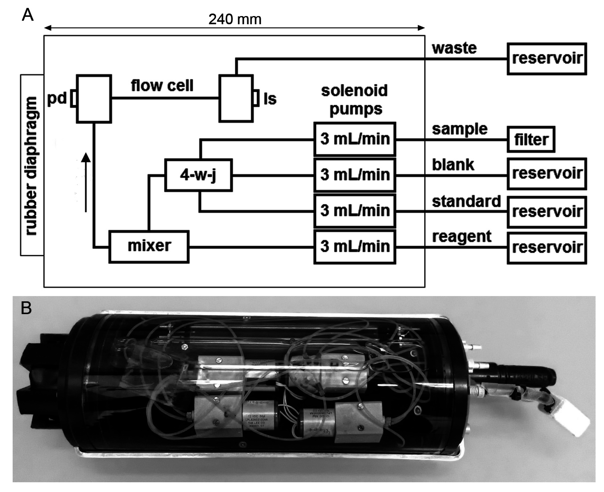
2.1. Apparatus
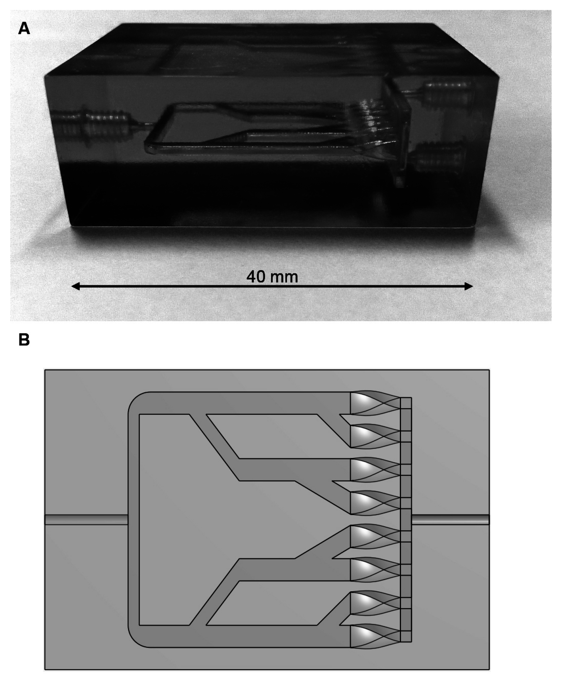
2.2. Flow Cell
2.3. Mixing Cell
2.4. Reagents
2.5. Chemical and Physical Parameters
3. Study Area
4. Results and Discussion
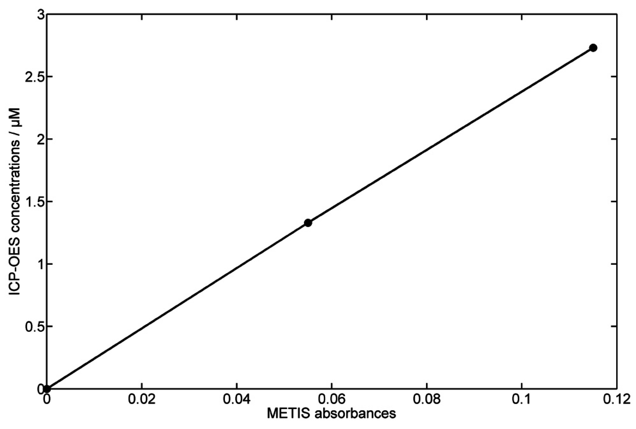
4.1. Calibration
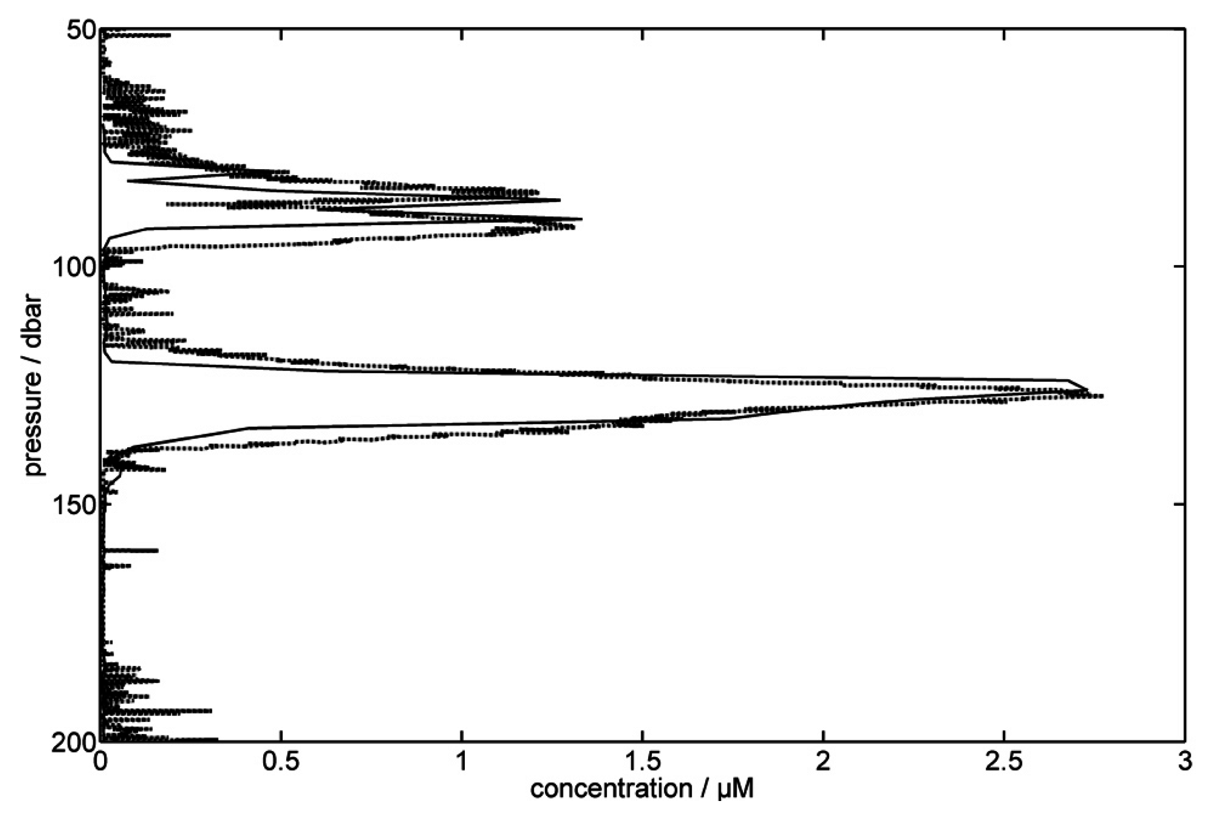
4.2. Mn(II) Analysis in the Baltic Sea
5. Conclusions
Acknowledgments
Author Contributions
Conflicts of Interest
References
- Tebo, B.M.; Bargar, J.R.; Dick, B.G.C.G.J.; Murray, K.J.; Parker, D.; Verity, R.; Webb, S.M. Biogenic Manganese Oxides: Properties and Mechanisms of Formation. Annu. Rev. Earth Planet. Sci. 2004, 32, 287–328. [Google Scholar] [CrossRef]
- Ho, T.Y.; Quigg, A.; Finkel, Z.V.; Milligan, A.J.; Wyman, K.; Falkowski, P.G.; Morel, F.M. The elemental composition of some marine phytoplankton. J. Phycol. 2003, 39, 1145–1159. [Google Scholar] [CrossRef]
- Crowley, J.D.; Traynor, D.A.; Weatherburn, D. Enzymes and proteins containing manganese: An overview. Met. Ions Biol. Syst. 2000, 37, 209–278. [Google Scholar] [PubMed]
- Kehres, D.G.; Maguire, M.E. Emerging themes in manganese transport, biochemistry and pathogenesis in bacteria. FEMS Microbiol. Rev. 2003, 27, 263–290. [Google Scholar] [CrossRef]
- Brand, L.E.; Sunda, W.G.; Guillard, R.R. Limitation of marine phytoplankton reproductive rates by zinc, manganese, and iron. Limnol. Oceanogr. 1983, 28, 1182–1198. [Google Scholar] [CrossRef]
- Coale, K.H. Effects of iron, manganese, copper, and zinc enrichments on productivity and biomass in the subarctic Pacific. Limnol. Oceanogr. 1991, 36, 1851–1864. [Google Scholar] [CrossRef]
- Johnson, K.S.; Coale, K.H.; Berelson, W.M.; Gordon, R.M. On the formation of the manganese maximum in the oxygen minimum. Geochim. Cosmochim. Acta 1996, 60, 1291–1299. [Google Scholar] [CrossRef]
- Luther, G.W.; Sundby, B.; Lewis, B.L.; Brendel, P.J.; Silverberg, N. Interactions of manganese with the nitrogen cycle: Alternative pathways to dinitrogen. Geochim. Cosmochim. Acta 1997, 61, 4043–4052. [Google Scholar] [CrossRef]
- Pohl, C.; Hennings, U. The effect of redox processes on the partitioning of Cd, Pb, Cu and Mn between dissolved and particulate phases in the Baltic Sea. Mar. Chem. 1999, 65, 41–53. [Google Scholar] [CrossRef]
- Dellwig, O.; Leipe, T.; März, C.; Glockzin, M.; Pollehne, F.; Schnetger, B.; Yakushev, E.V.; Böttcher, M.E.; Brumsack, H.J. A new particulate Mn-Fe-P-shuttle at the redoxcline of anoxic basins. Geochim. Cosmochim. Acta 2010, 74, 7100–7115. [Google Scholar] [CrossRef]
- Turnewitsch, R.; Pohl, C. An estimate of the efficiency of the iron- and manganese-driven dissolved inorganic phosphorus trap at an oxic/euxinic water column redoxcline. Glob. Biogeochem. Cycles 2010, 24, 1–15. [Google Scholar] [CrossRef]
- Van Cappellen, P.; Wang, Y. Cycling of iron and manganese in surface sediments: A general theory for the coupled transport and reaction of carbon, oxygen, nitrogen, sulfur, iron, and manganese. Am. J. Sci. 1996, 296, 197–243. [Google Scholar] [CrossRef]
- Huckriede, H.; Meischner, D. Origin and environment of manganese-rich sediments within black-shale basins. Geochim. Cosmochim. Acta 1996, 60, 1399–1413. [Google Scholar] [CrossRef]
- Pakhomova, S.V.; Hall, P.O.J.; Kononets, M.Y.; Rozanov, A.G.; Tengberg, A.; Vershinin, A.V. Fluxes of iron and manganese across the sediment-water interface under various redox conditions. Mar. Chem. 2007, 107, 319–331. [Google Scholar] [CrossRef]
- Dellwig, O.; Bosselmann, K.; Kölsch, S.; Hentscher, M.; Hinrichs, J.; Böttcher, M.E.; Reuter, R.; Brumsack, H.J. Sources and fate of manganese in a tidal basin of the German Wadden Sea. J. Sea Res. 2007, 57, 1–18. [Google Scholar] [CrossRef]
- Overnell, J.; Brand, T.; Bourgeois, W.; Statham, P.J. Manganese Dynamics in the Water Column of the Upper Basin of Loch Etive, a Scottish Fjord. Estuar. Coastal Shelf Sci. 2002, 55, 481–492. [Google Scholar] [CrossRef]
- Neretin, L.N.; Pohl, C.; Jost, G.; Leipe, T.; Pollehne, F. Manganese cycling in the Gotland Deep, Baltic Sea. Mar. Chem. 2003, 82, 125–143. [Google Scholar] [CrossRef]
- Schippers, A.; Neretin, L.N.; Lavik, G.; Leipe, T.; Pollehne, F. Manganese(II) oxidation driven by lateral oxygen intrusions in the western Black Sea. Geochim. Cosmochim. Acta 2005, 69, 2241–2252. [Google Scholar] [CrossRef]
- Trouwborst, R.E.; Clement, B.G.; Tebo, B.M.; Glazer, B.T.; Luther, G.W., III. Soluble Mn(III) in Suboxic Zones. Science 2006, 313, 1955–1957. [Google Scholar] [CrossRef] [PubMed]
- Yakushev, E.; Pakhomova, S.; Sørenson, K.; Skei, J. Importance of the different manganese species in the formation of water column redox zones: Observations and modeling. Mar. Chem. 2009, 117, 59–70. [Google Scholar] [CrossRef]
- Dellwig, O.; Schnetger, B.; Brumsack, H.J.; Grossart, H.P.; Umlauf, L. Dissolved reactive manganese at pelagic redoxclines (part II): Hydrodynamic conditions for accumulation. J. Mar. Syst. 2012, 90, 31–41. [Google Scholar] [CrossRef]
- Schnetger, B.; Dellwig, O. Dissolved reactive manganese at pelagic redoxclines (part I): A method for determination based on field experiments. J. Mar. Syst. 2012, 90, 23–30. [Google Scholar] [CrossRef]
- Webb, S.M.; Dick, G.J.; Bargar, J.R.; Tebo, B.M. Evidence for the presence of Mn(III) intermediates in the bacterial oxidation of Mn(II). Proc. Natl. Acad. Sci. USA 2005, 102, 5558–5563. [Google Scholar] [CrossRef] [PubMed]
- Nico, P.S.; Zasoski, R.J. Mn(III) Center Availability as a Rate Controlling Factor in the Oxidation of Phenol and Sulfide on δMnO2. Environ. Sci. Technol. 2001, 35, 3338–3343. [Google Scholar] [CrossRef] [PubMed]
- Madison, A.S.; Tebo, B.M.; Luther, G.W. Simultaneous determination of soluble manganese (III), manganese (II) and total manganese in natural (pore) waters. Talanta 2011, 84, 374–381. [Google Scholar] [CrossRef] [PubMed]
- Stramma, L.; Johnson, G.C.; Sprintall, J.; Morholz, V. Expanding Oxygen-Minimum Zones in the Tropical Oceans. Science 2008, 320, 655–658. [Google Scholar] [CrossRef] [PubMed]
- Keeling, R.F.; Körtzinger, A.; Gruber, N. Ocean Deoxygenation in a Warming World. Annu. Rev. Mar. Sci. 2009, 2, 199–229. [Google Scholar] [CrossRef] [PubMed]
- Gruber, N. Warming up, turning sour, losing breath: Ocean biogeochemistry under global change. Philos. Trans. R. Soc. A 2011, 369, 1980–1996. [Google Scholar] [CrossRef] [PubMed]
- Klinkhammer, G.P. Fiber optic spectrometers for in-situ measurements in the oceans: The ZAPS Probe. Mar. Chem. 1994, 47, 13–20. [Google Scholar] [CrossRef]
- Okamura, K.; Gamo, T.; Obata, H.; Nakayama, E.; Karatani, H.; Nozaki, Y. Selective and sensitive determination of trace manganese in sea water by flow through technique using luminol-hydrogen peroxide chemiluminescence detection. Anal. Chim. Acta 1998, 377, 125–131. [Google Scholar] [CrossRef]
- Tercier-Waeber, M.L.; Belmont-Hébert, C.; Buffle, J. Real-time continuous Mn (II) monitoring in lakes using a novel voltammetric in situ profiling system. Environ. Sci. Technol. 1998, 32, 1515–1521. [Google Scholar] [CrossRef]
- Luther, G.W.; Glazer, B.T.; Ma, S.; Trouwborst, R.E.; Moore, T.S.; Metzger, E.; Kraiya, C.; Waite, T.J.; Druschel, G.; Sundby, B.; et al. Use of voltammetric solid-state (micro) electrodes for studying biogeochemical processes: Laboratory measurements to real time measurements with an in situ electrochemical analyzer (ISEA). Mar. Chem. 2008, 108, 221–235. [Google Scholar] [CrossRef] [Green Version]
- Chin, C.S.; Johnson, K.S.; Coale, K.H. Spectrophotometric determination of dissolved manganese in natural waters with 1-(2-pyridylazo)-2-naphthol: Application to analysis in situ in hydrothermal plumes. Mar. Chem. 1992, 37, 65–82. [Google Scholar] [CrossRef]
- Resing, J.A.; Mottl, M.J. Determination of manganese in seawater using flow injection analysis with on-line preconcentration and spectrophotometric detection. Anal. Chem. 1992, 64, 2682–2687. [Google Scholar] [CrossRef]
- Chin, C.S.; Coale, K.H.; Elrod, V.A.; Johnson, K.S. In situ observations of dissolved iron and manganese in hydrothermal vent plumes, Juan de Fuca Ridge. J. Geophys. Res. 1994, 99, 4969–4984. [Google Scholar] [CrossRef]
- Massoth, G.J.; Baker, E.T.; Feely, R.A.; Lupton, J.E.; Collier, R.W.; Gendron, J.F.; Roe, K.K.; Maenner, S.M.; Resing, J.A. Manganese and iron in hydrothermal plumes resulting from the 1996 Gorda Ridge Event. Deep Sea Res. Part II 1998, 45, 2683–2712. [Google Scholar] [CrossRef]
- Statham, P.J.; Connelly, D.P.; German, C.R.; Brand, T.; Overnell, J.O.; Bulukin, E.; Millard, N.; McPhail, S.; Pebody, M.; Perrett, J.; et al. Spatially Complex Distribution of Dissolved Manganese in a Fjord as Revealed by High-Resolution in Situ Sensing Using the Autonomous Underwater Vehicle Autosub. Environ. Sci. Technol. 2005, 39, 9440–9445. [Google Scholar] [CrossRef] [PubMed]
- Doi, T.; Takano, M.; Okamura, K.; Ura, T.; Gamo, T. In-situ Survey of Nanomolar Manganese in Seawater Using an Autonomous Underwater Vehicle around a Volcanic Crater at Teishi Knoll, Sagami Bay, Japan. J. Oceanogr. 2008, 64, 471–477. [Google Scholar] [CrossRef]
- Johnson, K.S.; Beehler, C.L.; Sakamoto-Arnold, C.M. A submersible flow analysis system. Anal. Chim. Acta 1986, 179, 245–257. [Google Scholar] [CrossRef]
- Massoth, G. A SUAVE (Submersible System Used to Assess Vented Emissions) approach to plume sensing: The Buoyant Plume Experiment at Cleft segment, Juan de Fuca Ridge and plume exploration along the EPR9-10 N. Eos 1991, 72, 234. [Google Scholar]
- Okamura, K.; Kimoto, H.; Saeki, K.; Ishibashi, J.; Obata, H.; Maruo, M.; Gamo, T.; Nakayama, E.; Nozaki, Y. Development of a deep-sea in situ Mn analyzer and its application for hydrothermal plume observation. Mar. Chem. 2001, 76, 17–26. [Google Scholar] [CrossRef]
- Luther, G.W., III; Reimers, C.E.; Nuzzio, D.B.; Lovalvo, D. In Situ Deployment of Voltammetric, Potentiometric, and Amperometric Microelectrodes from a ROV to Determine Dissolved O2, Mn, Fe, S(-2), and pH in Porewaters. Environ. Sci. Technol. 1999, 33, 4352–4356. [Google Scholar] [CrossRef]
- Milani, A.; Statham, P.J.; Mowlem, M.C.; Connelly, D.P. Development and application of a microfluidic in-situ analyzer for dissolved Fe and Mn in natural waters. Talanta 2015, 136, 15–22. [Google Scholar] [CrossRef] [PubMed]
- Okamura, K.; Hatanaka, H.; Kimoto, H.; Suzuki, M.; Sohrin, Y.; Nakayama, E.; Gamo, T.; Ishibashi, J.I. Development of an in situ manganese analyzer using micro-diaphragm pumps and its application to time-series observations in a hydrothermal field at the Suiyo seamount. Geochem. J. 2004, 38, 635–642. [Google Scholar] [CrossRef]
- Prien, R.D.; Connelly, D.P.; German, C. In Situ Chemical Analyser for the Determination of Dissolved Fe(II) and Mn(II). EOS Trans. AGU 2006, 87, OS44B-06. [Google Scholar]
- Prien, R.D.; Schulz-Bull, D.E. Technical note: GODESS - A profiling mooring in the Gotland Basin. Ocean Sci. 2016, 12, 899–907. [Google Scholar] [CrossRef]
- Liebig, J. Ueber Versilberung und Vergoldung von Glas. Justus Liebigs Annalen der Chemie 1856, 98, 132–139. (In German) [Google Scholar] [CrossRef]
- Cheng, K.L.; Bray, R.H. 1-(2-Pyridylazo)-2-naphthol as a Possible Analytical Reagent. Anal. Chem. 1955, 27, 782–785. [Google Scholar] [CrossRef]
- Cheng, K.L.; Ueno, K. Handbook of Organic Analytical Reagents; CRC Press: Boca Raton, FL, USA, 1982. [Google Scholar]
- Chiswell, B.; Rauchle, G.; Pascoe, M. Spectrophotometric methods for the determination of manganese. Talanta 1990, 37, 237–259. [Google Scholar] [CrossRef]
- Goto, K.; Taguchi, S.; Fukue, Y.; Ohta, K.; Watanabe, H. Spectrophotometric determination of manganese with 1-(2-pyridylazo)-2-naphthol and a non-ionic surfactant. Talanta 1977, 24, 752–753. [Google Scholar] [CrossRef]
- Mesmer, R.; Baes, C., Jr.; Sweeton, F. Acidity measurements at elevated temperatures. VI. Boric acid equilibriums. Inorg. Chem. 1972, 11, 537–543. [Google Scholar] [CrossRef]
- Feng, S.; Huang, Y.; Yuan, D.; Zhu, Y.; Zhou, T. Development and application of a shipboard method for spectrophotometric determination of trace dissolved manganese in estuarine and coastal waters. Cont. Shelf Res. 2015, 92, 37–43. [Google Scholar] [CrossRef]
- Strady, E.; Pohl, C.; Yakushev, E.V.; Krüger, S.; Hennings, U. PUMP–CTD-System for trace metal sampling with a high vertical resolution. A test in the Gotland Basin, Baltic Sea. Chemosphere 2008, 70, 1309–1319. [Google Scholar] [CrossRef] [PubMed]
- Cline, J. Spectrophotometric determination of hydrogen sulfide in natural waters. Limnol. Oceanogr. 1969, 14, 454–458. [Google Scholar] [CrossRef]
- Feistel, R.; Nausch, G.; Matthaus, W.; Hagen, E. Temporal and spatial evolution of the Baltic deep water renewal in Spring 2003. Oceanologia 2003, 45, 623–642. [Google Scholar]
- Matthäus, W.; Schinke, H. The influence of river runoff on deep water conditions of the Baltic Sea. Hydrobiologia 1999, 393, 1–10. [Google Scholar] [CrossRef]
- Elken, J.; Matthäus, W. Baltic Sea oceanography. In Assessment of Climate Change for the Baltic Sea Basin; Regional Climate Studies; Springer: Berlin/Heidelberg, Germany, 2008; Volume 1, pp. 379–385. [Google Scholar]
- Mohrholz, V.; Naumann, M.; Nausch, G.; Krüger, S.; Gräwe, U. Fresh oxygen for the Baltic Sea: An exceptional saline inflow after a decade of stagnation. J. Mar. Syst. 2015, 148, 152–166. [Google Scholar] [CrossRef]
- Statham, P.J.; Connelly, D.P.; German, C.R.; Bulukin, E.; Millard, N.; McPhail, S.; Pebody, M.; Perrett, J.; Squires, M.; Stevenson, P.; et al. Mapping the 3D spatial distribution of dissolved manganese in coastal waters using an in situ analyser and the autonomous underwater vehicle Autosub. Underw. Technol. 2003, 25, 129–134. [Google Scholar] [CrossRef]
- Diaz, R.J.; Rosenberg, R. Spreading Dead Zones and Consequences for Marine Ecosystems. Science 2008, 321, 926–929. [Google Scholar] [CrossRef] [PubMed]
- Piker, L.; Schmaljohann, R.; Imhoff, J.F. Dissimilatory sulfate reduction and methane production in Gotland Deep sediments (Baltic Sea) during a transition period from oxic to anoxic bottom water (1993–1996). Aquat. Microbiol. Ecol. 1998, 14, 183–193. [Google Scholar] [CrossRef] [Green Version]
- Zillén, L.; Conley, D.J.; Andrén, T.; Andrén, E.; Björck, S. Past occurrences of hypoxia in the Baltic Sea and the role of climate variability, environmental change and human impact. Earth-Sci. Rev. 2008, 91, 77–92. [Google Scholar] [CrossRef]
- Pohl, C.; Hennings, U. The coupling of long-term trace metal trends to internal trace metal fluxes at the oxic–Anoxic interface in the Gotland Basin (57°19,20′ N; 20°03,00′ E) Baltic Sea. J. Mar. Syst. 2005, 56, 207–225. [Google Scholar] [CrossRef]
- Lewis, B.L.; Landing, W.M. The biogeochemistry of manganese and iron in the Black Sea. Deep-Sea Res. 1991, 38, 773–803. [Google Scholar] [CrossRef]
- Holtermann, P.L.; Umlauf, L.; Tanhua, T.; Schmale, O.; Rehder, G.; Waniek, J.J. The Baltic Sea Tracer Release Experiment: 1. Mixing rates. J. Geophys. Res. 2012, 117, C01021. [Google Scholar] [CrossRef]
- Tebo, B.M. Manganese (II) oxidation in the suboxic zone of the Black Sea. Deep-Sea Res. Part A 1991, 38, S883–S905. [Google Scholar] [CrossRef]
- Stüben, D.; Stoffers, P.; Cheminée, J.L.; Hartmann, M.; McMurtry, G.M.; Richnow, H.H.; Jenisch, A.; Michaelis, W. Manganese, methane, iron, zinc, and nickel anomalies in hydrothermal plumes from Teahitia and Macdonald volcanoes. Geochim. Cosmochim. Acta 1992, 56, 3693–3704. [Google Scholar] [CrossRef]
- Lee, D.Y.; Owens, M.S.; Doherty, M.; Eggleston, E.M.; Hewson, I.; Crump, B.C.; Cornwell, J.C. The effects of oxygen transition on community respiration and potential chemoautotrophic production in a seasonally stratified anoxic estuary. Estuaries Coasts 2015, 38, 104–117. [Google Scholar] [CrossRef]


© 2016 by the authors; licensee MDPI, Basel, Switzerland. This article is an open access article distributed under the terms and conditions of the Creative Commons Attribution (CC-BY) license (http://creativecommons.org/licenses/by/4.0/).
Share and Cite
Meyer, D.; Prien, R.D.; Dellwig, O.; Waniek, J.J.; Schuffenhauer, I.; Donath, J.; Krüger, S.; Pallentin, M.; Schulz-Bull, D.E. A Multi-Pumping Flow System for In Situ Measurements of Dissolved Manganese in Aquatic Systems. Sensors 2016, 16, 2027. https://doi.org/10.3390/s16122027
Meyer D, Prien RD, Dellwig O, Waniek JJ, Schuffenhauer I, Donath J, Krüger S, Pallentin M, Schulz-Bull DE. A Multi-Pumping Flow System for In Situ Measurements of Dissolved Manganese in Aquatic Systems. Sensors. 2016; 16(12):2027. https://doi.org/10.3390/s16122027
Chicago/Turabian StyleMeyer, David, Ralf D. Prien, Olaf Dellwig, Joanna J. Waniek, Ingo Schuffenhauer, Jan Donath, Siegfried Krüger, Malte Pallentin, and Detlef E. Schulz-Bull. 2016. "A Multi-Pumping Flow System for In Situ Measurements of Dissolved Manganese in Aquatic Systems" Sensors 16, no. 12: 2027. https://doi.org/10.3390/s16122027
APA StyleMeyer, D., Prien, R. D., Dellwig, O., Waniek, J. J., Schuffenhauer, I., Donath, J., Krüger, S., Pallentin, M., & Schulz-Bull, D. E. (2016). A Multi-Pumping Flow System for In Situ Measurements of Dissolved Manganese in Aquatic Systems. Sensors, 16(12), 2027. https://doi.org/10.3390/s16122027