Node Self-Deployment Algorithm Based on Pigeon Swarm Optimization for Underwater Wireless Sensor Networks

College of Automation, Hangzhou Dianzi University, Hangzhou 310018, China
*
Author to whom correspondence should be addressed.
Sensors 2017, 17(4), 674; https://doi.org/10.3390/s17040674
Submission received: 19 January 2017
/
Revised: 20 March 2017
/
Accepted: 20 March 2017
/
Published: 24 March 2017
(This article belongs to the Special Issue Advances and Challenges in Underwater Sensor Networks)
Abstract
:At present, free-to-move node self-deployment algorithms aim at event coverage and cannot improve network coverage under the premise of considering network connectivity, network reliability and network deployment energy consumption. Thus, this study proposes pigeon-based self-deployment algorithm (PSA) for underwater wireless sensor networks to overcome the limitations of these existing algorithms. In PSA, the sink node first finds its one-hop nodes and maximizes the network coverage in its one-hop region. The one-hop nodes subsequently divide the network into layers and cluster in each layer. Each cluster head node constructs a connected path to the sink node to guarantee network connectivity. Finally, the cluster head node regards the ratio of the movement distance of the node to the change in the coverage redundancy ratio as the target function and employs pigeon swarm optimization to determine the positions of the nodes. Simulation results show that PSA improves both network connectivity and network reliability, decreases network deployment energy consumption, and increases network coverage.
1. Introduction
Underwater wireless sensor networks (UWSNs) are network-monitoring systems in an underwater environment. The sensor nodes in these networks have perceptual, acoustic communication, and computational capabilities, and they can transmit the sensed information to the sink node for processing and analysis by one-hop or multi-hop methods [1,2]. UWSNs have been applied to water environment monitoring, underwater resource exploration, and marine military defense [3,4]. Research on UWSNs [5] mainly involves network architecture design [6], node deployment, node localization [7,8], time synchronization [9], network protocol design [10,11], etc. As the first step in UWSNs application, node deployment significantly affects network service in different aspects, including network coverage, network connectivity, and network energy consumption. The node-deployment problem is defined that move sensor nodes to the corresponding positions in an artificial or a self-organized manner to form a network topology that has special characteristics and increases the network service [4,12]. Meanwhile, the goals of node deployment are to increase network coverage and network connectivity, decrease network energy consumption, and prolong network lifetime. Generally, the problem of node deployment can be divided into static deployment, move-restricted node self-deployment, and free-to-move node self-deployment according to the mobility of the node [2,13,14,15,16,17]. In static deployment, the nodes cannot move and are deployed in the target area by the artificial method [14]. Thus, static deployment is not appropriate for the large-scale deployment. In move-restricted node self-deployment, the nodes can move only vertically and adjust their depth by themselves according to the local information near the node [18]. In free-to-move node self-deployment, the nodes have the capability to move freely in all directions [19]. With the improvement of the design level of the sensor node, the cost of the mobile nodes is reduced and more and more scholars concentrate on the research of free-to-move node self-deployment. Moreover, free-to-move node self-deployment is closer to the reality. Therefore, free-to-move node self-deployment has wide application scenarios and has important research significance.
The existing free-to-move node self-deployment algorithms [20,21,22,23,24,25] usually regard the event coverage as the research object, and aim at the network coverage, but these algorithms do not regard the network connectivity and network reliability as the goal simultaneously. Furthermore, in these algorithms, each node should move several rounds to determine the final deployed position, which increases the network deployment energy consumption. Consequently, there is still much space to improve the performance of free-to-move node self-deployment algorithms.
Thus, the current paper proposes the pigeon-based self-deployment algorithm (PSA) to solve these problems. The sink node first finds its one-hop nodes and maximizes the coverage in its one-hop region. This process allows for the maintenance of the number of the nodes deployed in the region near the sink node and increases network reliability and network coverage as much as possible. The one-hop nodes then divide the network into layers and cluster in every layer. This mechanism forms a distribution in which the scale of the cluster is small and the number of cluster head nodes is great in the region close to the sink node. The cluster head nodes do not move again, thus, the number of nodes in the region close to the sink node increases. Each cluster head node subsequently constructs a connected path to the sink node to guarantee network connectivity. Finally, the cluster head node regards the ratio of the movement distance of a cluster-in node to the change in the coverage redundancy ratio (CRR) of the node as the target function on the premise that the cluster-in node should be connected to the cluster head node by one-hop or multi-hop path. Pigeon swarm optimization is then employed to solve the moving position of the node. This method can determine the optimal deployment location in the continuous solution space, and minimize the complexity of the search for the optimal deployment location. Moreover, the moving position of each node can be determined at once, which can reduce the deployment energy consumption. PSA is compared with the three-dimensional virtual forces deployment algorithm (TVFDA) [25] in terms of network coverage, network connectivity, network reliability and energy consumption. The simulation results show that PSA increases both network connectivity and network reliability, decreases network energy consumption, and increases network coverage.
The rest of this paper is organized as follows: Section 2 introduces the related work about free-to-move node self-deployment. Section 3 describes the system model, preliminaries, and definitions considered in this study. Section 4 presents details of PSA. Section 5 analyses the complexity of PSA. Section 6 discusses the performance study and provides a detailed analysis of its result. Finally, Section 7 concludes the paper and presents future research directions.
2. Related Work
Some scholars have recently developed free-to-move node self-deployment algorithms for UWSNs. Wang et al. [20,21] proposed three kinds of movement-assisted sensor deployment algorithms, namely, vector-based algorithm, Voronoi-based algorithm, and Minimax algorithm. These three algorithms are all based on the Voronoi diagram. In the vector-based algorithm, a node moves to the next position according to the repulsive force exerted on the node by its Voronoi neighbor nodes. In the Voronoi-based algorithm, a node moves to the farthest vertex of its Voronoi diagram every round. In the Minimax algorithm, a node moves closer to the farthest vertex of its Voronoi diagram to avoid the situation in which a vertex that was originally close becomes the new farthest vertex. In these algorithms, each node can move autonomously to the corresponding position to cover the coverage hole according to its own local information. Thus, these algorithms can increase network coverage, and meet the distributed characteristic of the sensor network. However, the Voronoi diagram of each node should be formed in each of the iterations, and this process requires each node to know the global information of the network and consequently results in extra communication energy consumption. Moreover, the process based on the 3D Voronoi diagram of the node is more complex compared with that based on 2D Voronoi diagram. Thus, these algorithms are suitable for 2D node self-deployment but unsuitable for node self-deployment in UWSNs. Koutsougeras et al. [22] proposed a sensor deployment algorithm based on self-organizing maps for the event. In each of the iterations, an event is selected by a random sequence, and the node that is closest to the event should update its position according to the rule of movement. The node moves a certain distance to the event, and the distance of the movement is proportional to the distance between the node and the event. The algorithm is iterated until no more significant movement is possible. This algorithm can deploy the node according to the density of the event in the region and accomplish an uneven deployment in the target area. However, this algorithm adjusts the node position by the centralized way, which is difficult to achieve in practice. Xia et al. [23] proposed a fish swarm-inspired underwater sensor deployment algorithm (FSSDA). Drawing on the foraging behavior of the fish swarm, this algorithm regards the node as the fish and the event as the food, moves the node to cover the event, and finally completes the deployment for the event according to the crowding parameter of each event. The algorithm has low computational complexity and rapid convergence rate. Du et al. [24] proposed a particle swarm-inspired underwater sensor self-deployment algorithm. The process of the node deployment in the algorithm is similar to that in FSSDA, but the algorithm also considers the situation in which the position of the event is dynamically changing, like the situation in practice. However, both algorithms are suitable for the distributed coverage of the event but unsuitable for the coverage of the region. In addition, these algorithms also ignore network connectivity. Li et al. [25] proposed a three-dimensional virtual forces deployment algorithm (TVFDA). This algorithm applies the concepts of gravitation and repulsion in physics to the wireless sensor network and considers that these forces exist between nodes in the network. Therefore, in the algorithm, each node moves to the next position according to the join forces, which are exerted on the node by its neighbor nodes, and each node stops moving until its join forces is zero or the maximum iteration number is reached. This algorithm allows for an even distribution of the nodes in the target area compared with situation before the algorithm is run; thus, this algorithm enhances network coverage and meets the characteristics of underwater wireless sensor networks. However, in this virtual force algorithm, each node needs to know the related information of its neighbors in each iteration, that is, each node should communicate with its neighbor nodes in each iteration; thus, this algorithm results in increased network energy consumption. Moreover, each node should move a real distance several times according to the gravitational and repulsive forces exerted on it. Consequently, this algorithm may segment the network, degrade network connectivity, and increase network energy consumption for the node deployment. Furthermore, being incapable of controlling the number of the nodes in the region near the sink node, TVFDA may degrade both network reliability and energy efficiency.
3. Preliminaries, Models, and Definitions
3.1. Preliminaries
N nodes are thrown in the target area (rectangular or cubic) uniformly and randomly. Each node then moves to the determined position with the aid of an autonomous underwater vehicle (AUVs), and each node is fixed at the position by an anchor after its deployment position is calculated by the deployment algorithm. In addition, sensor nodes communicate with one another through acoustic channels and maintain connectivity with the sink node via one-hop or multi-hop paths. The following assumptions are made:
- (1)
- A node adopts the Boolean sensing model [26], and the sensing radius of the node is fixed.
- (2)
- All nodes have the same states, including initial energy, sensing radius, and communication radius, before the node deployment. Moreover, the communication radius of the node can be adjusted according to the demand of the algorithm but should not exceed the maximum communication radius, which is determined by the physical device during the node deployment.
- (3)
- With the similar assumptions in [24] as inspiration, the sink node is fixed at the center of the water face. By contrast, the other nodes can move freely in all directions, and their real-time locations can be determined using a localization algorithm or global positioning satellite devices during the node deployment.
3.2. Related Models
3.2.1. Coverage Redundancy Ratio
The coverage redundancy ratio (CRR) of the node (i.e., si) is defined as the ratio of the sensing area of the node with its neighbor node (i.e., the node within si’s maximum communication radius) to si’s sensing area [27]. CRR is formulated as follows [27]:
where n is the number of the neighbor nodes of node si and d(si,sj) is the distance between node si and its neighbor node sj.
3.2.2. Underwater Energy Consumption
During the node deployment, each node should determine the local information near its position by communicating with its neighbor nodes, and each node should move to the determined position when it knows the position. Therefore, the energy consumption in this study is divided into communication energy consumption and deployment energy consumption.
(1) Communication Energy Consumption
The nodes of an underwater sensor network communicate with one another by acoustic signals [28]. Thus, the communication energy consumption of the acoustic medium [29] is adopted in this study and given by
This expression describes the energy consumption when the data packet is transmitted from the sending node to the receiving node. In Equation (2), Pr is the minimum number of power packets that can be received, and Tp is the data transmission time, whose formulation is as follows:
where Lb is the length of the sent data packet and Vt is the transmission speed of the data packet in water. The energy attenuation during the transmission of the data packet at a given distance is described as follows:
where λ is the energy diffusion factor, whose value is generally equal to 1.5, and α is a parameter determined by the following expression:
In Equation (5), a(Fr) is the absorption coefficient (in dB/m) formulated as follows:
where Fr is the carrier frequency in kHz.
(2) Deployment Energy Consumption
In the process of the node self-deployment for underwater wireless sensor networks, each node moves to the determined position that the node self-deployment algorithm calculates. The energy consumption because of node moving in the process is called the deployment energy consumption. Because the methods of nodes moving are various, it is difficult to express with a specific model. Therefore, in the problem of node deployment, the total distance of all nodes in the deployment process is used to measure the deployment energy consumption of a node deployment algorithm.
3.3. Definitions
3.3.1. Network Coverage
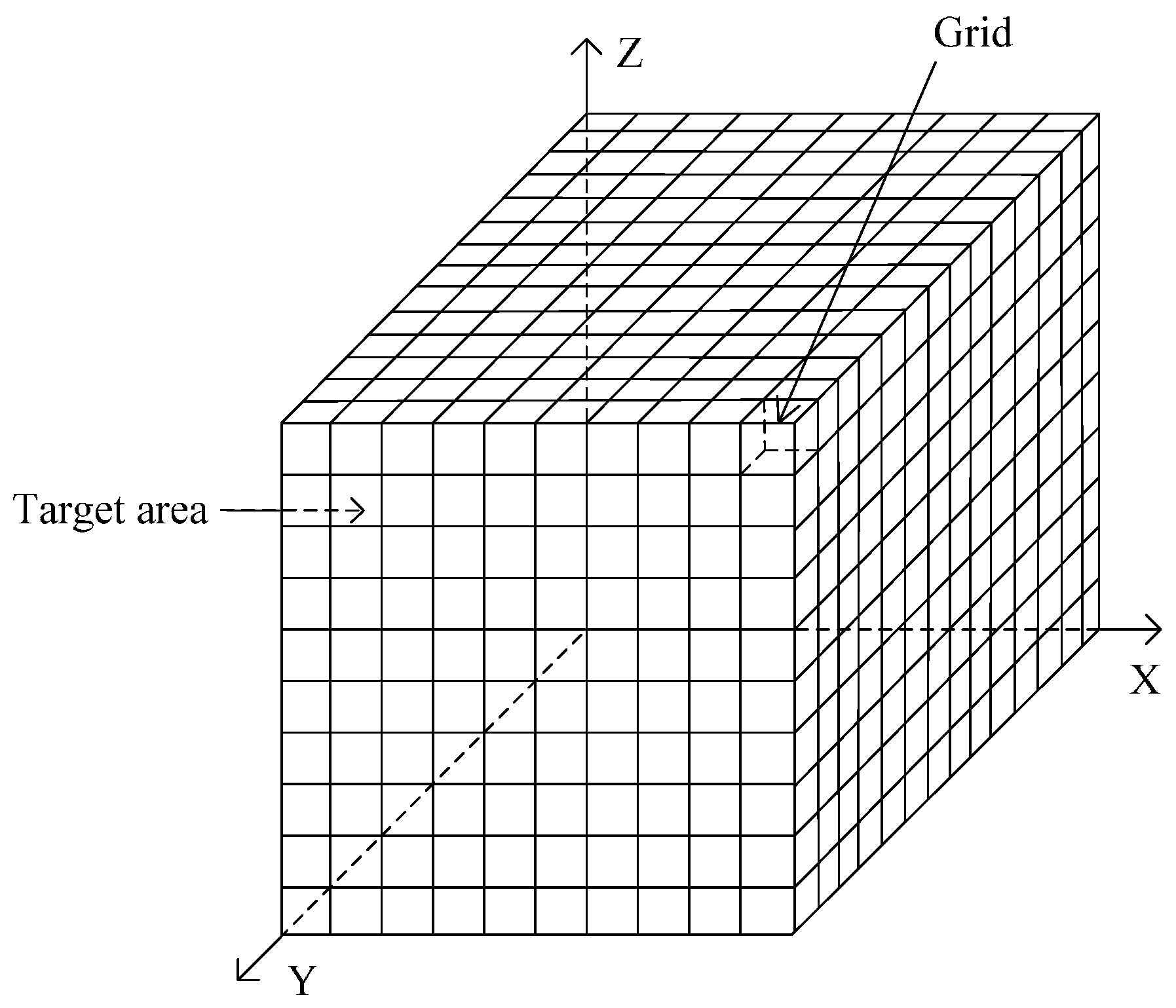
An underwater 3D space (target coverage area) is usually represented by a cuboid or cube. This space is divided into a number of small cubic grids whose sides have the length w [18]. The center of each cubic grid called the grid point, which is regarded as the representative of the grid. Each grid point has its own coordinates. A typical underwater 3D space is illustrated in Figure 1.
Network coverage, which reflects the degree an underwater sensor network covers a monitoring or target area, is a primary criterion parameter in the evaluation of a node-deployment algorithm. This parameter is defined as the ratio of the number of grid points covered by UWSNs to the total number of grid points in the target area. Network coverage is denoted by rcov, whose formula is as follows:
where Ncov is the number of grid points covered by the active nodes and Ntotal is the total number of grid points in the target area.
3.3.2. Network Connectivity
Network connectivity is another important criterion parameter for evaluating the quality of service in sensor networks. This parameter is a prerequisite for the effective application of sensor networks. It is defined as the ratio of the number of nodes connected to the sink node by a one-hop or multi-hop path to the total number of nodes in the network. The number of nodes connected to the sink node can be calculated by breadth-first search, in which the sink node is the root node.
4. Problem and Algorithm Description
4.1. Problem Description
The existing free-to-move node self-deployment algorithms usually aim at the event coverage and deploy the node according to the network coverage. However, these algorithms do not consider the problems related to network connectivity, network reliability, and network energy consumption. Furthermore, these algorithms determine the final position of each node after the node moves several rounds according to the result of every iteration of the algorithm. This process induces each node to move to the final position not in a straight line, thereby increasing the moving distance of the node and the energy consumption. In these algorithms, the network coverage is increased by forcing each node to move an appropriate distance in each of the iterations so that the node can stay away from each other as far as possible. This process decreases the area of the overlapping region in the target area; however, the probability of deploying the node near the sink node is also decreased. As a result, holes appear in the locations near the sink node more easily, and the network service may be degraded regardless of the network routing protocol. In addition, positioning the nodes far from other nodes, may lead to a segmented network, which detrimentally also affects network connectivity. Thus, in this study, the problem is defined as follows: given N sensor nodes that are thrown randomly and uniformly in the deployment space, design an algorithm to maximize network coverage, maintain network connectivity while minimizing energy consumption.
This study proposes the pigeon-based self-deployment algorithm (PSA) for UWSNs to solve the drawbacks of the existing free-to-move node self-deployment algorithms. In PSA, the sink node first finds its one-hop nodes and maximizes network coverage in its one-hop region. The one-hop nodes then divide the network into layers and cluster in each layer. Each cluster head node constructs a connected path to the sink node to guarantee network connectivity. Finally, each cluster head node regards the ratio of the movement distance of the node to the change in CRR of the node as the target function and uses pigeon swarm optimization to solve its position. As a result, the network coverage is expanded, the deployment energy consumption is reduced, and the number of node in the region near the sink node is increased.
4.2. Algorithm Description
4.2.1. Pigeon Swarm Optimization Algorithm
The pigeon swarm optimization algorithm (PSOA) is proposed by Duan and Quiao [30,31] in 2014. The algorithm is derived from the behavior of homing pigeons. PSOA consists of two models, namely, the map and compass operator and the landmark operator. PSOA has better optimization performance and faster convergence speed, comparing with other artificial intelligence algorithms [32,33].
(1) Map and Compass Operator
When all the pigeons are not familiar with the destination or landmark during the initialization of the algorithm, they determine the flying position and direction according to the magnetic field and the position of the sun. In this model, each pigeon updates its position according to the recent global optimal solution in the current iteration. On the assumption that the position and speed of the j-th pigeon are Xj and Vj, respectively, Xj and Vj are updated according to Equations (8) and (9) in the t-th iteration.
where G is the map and compass factor, rand is a random number, and Xg is the global optimal position in the t-th iteration.
(2) Landmark Operator
After PSOA has run for some time, some pigeons may have found the destination or familiar landmarks. Thus, these pigeons can move to the destination quickly, and the others move behind them. On the assumption that Xc(t) is the center of the position of the pigeon whose fitness is the top Np/2, the position of each pigeon in the t-th iteration is
where Np(t) is the number of pigeons that meets the restriction of the condition in the t-th iteration and fitness(Xj(t)) is the proportion of the fitness of the j-th pigeon to that of all the pigeons. In the minimum optimization problem, the fitness is formulated as follows:
where, f is the fitness function andis a small value.
4.2.2. PSA Process Description
The process of PSA is divided into three stages: (1) deploying in the one-hop region of the sink node; (2) network layering and clustering; and (3) optimizing the position of the cluster-in nodes.
(1) Deploying in the one-hop region of the sink node
After the nodes are thrown in the target area uniformly and randomly, the sink node broadcasts “beginning deployment” information with the communication radius, . The node receiving the information (i.e., si) confirms the sink node as its next hop node and relays its location information, poriginal(si):
These nodes are called the one-hop nodes of the sink node, or the one-hop node SH. |SH| is the number of elements in the set of one-hop nodes. The sink node then optimizes the network coverage in the one-hop region of the sink node. The ratio of the deployment energy consumption for moving the node to the final position, pdeployed(si), to the difference between CRR in poriginal(si) and pdeployed(si) is regarded as the fitness function fitness1:
where cborder is a constant expressing the minimum distance between the deployment position of the node and the boundary of the target area.
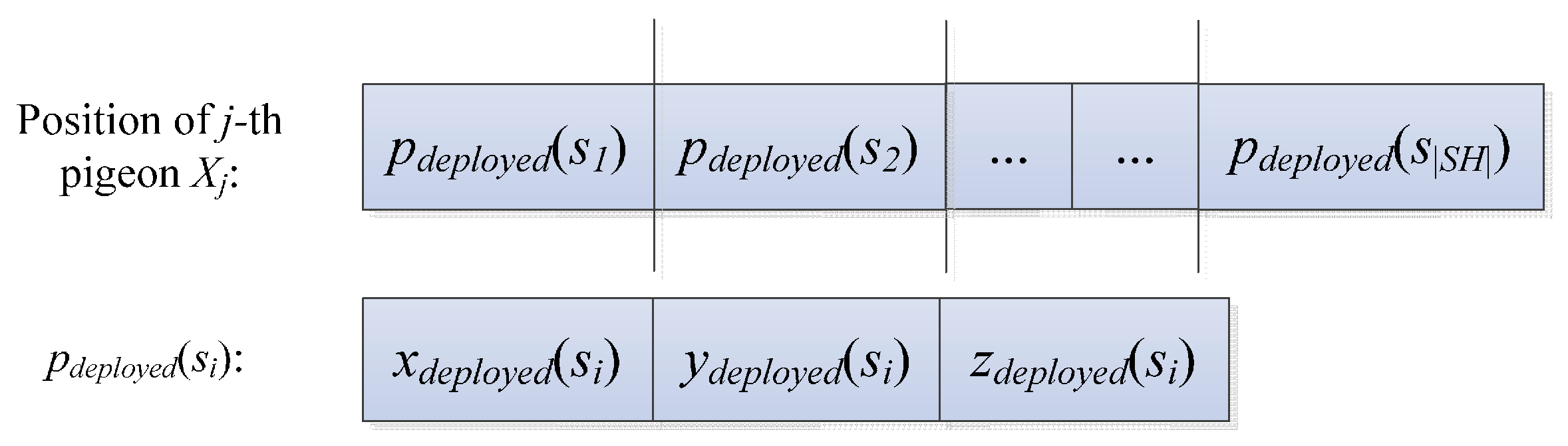
The number of the pigeons is set to Np, and the positions of the pigeons are initialized. The position of the j-th pigeon, Xj, consists of the coordinates of |SH| random points, each of which represents the position of a node in the set SH. These random nodes are in the hemisphere that regards the sink node as the center of the sphere. These nodes also regard the radius of the sphere to be 1.25 times that of the minimum communication radius. Thus, Xj is illustrated in Figure 2.
Subsequently, the solution of fitness1, Xg, is calculated according to the PSOA described in Section 4.2.1, and the position of node si is formulated as follows:
(2) Network Layering and Clustering
This stage is further divided into four steps.
- Step 1.
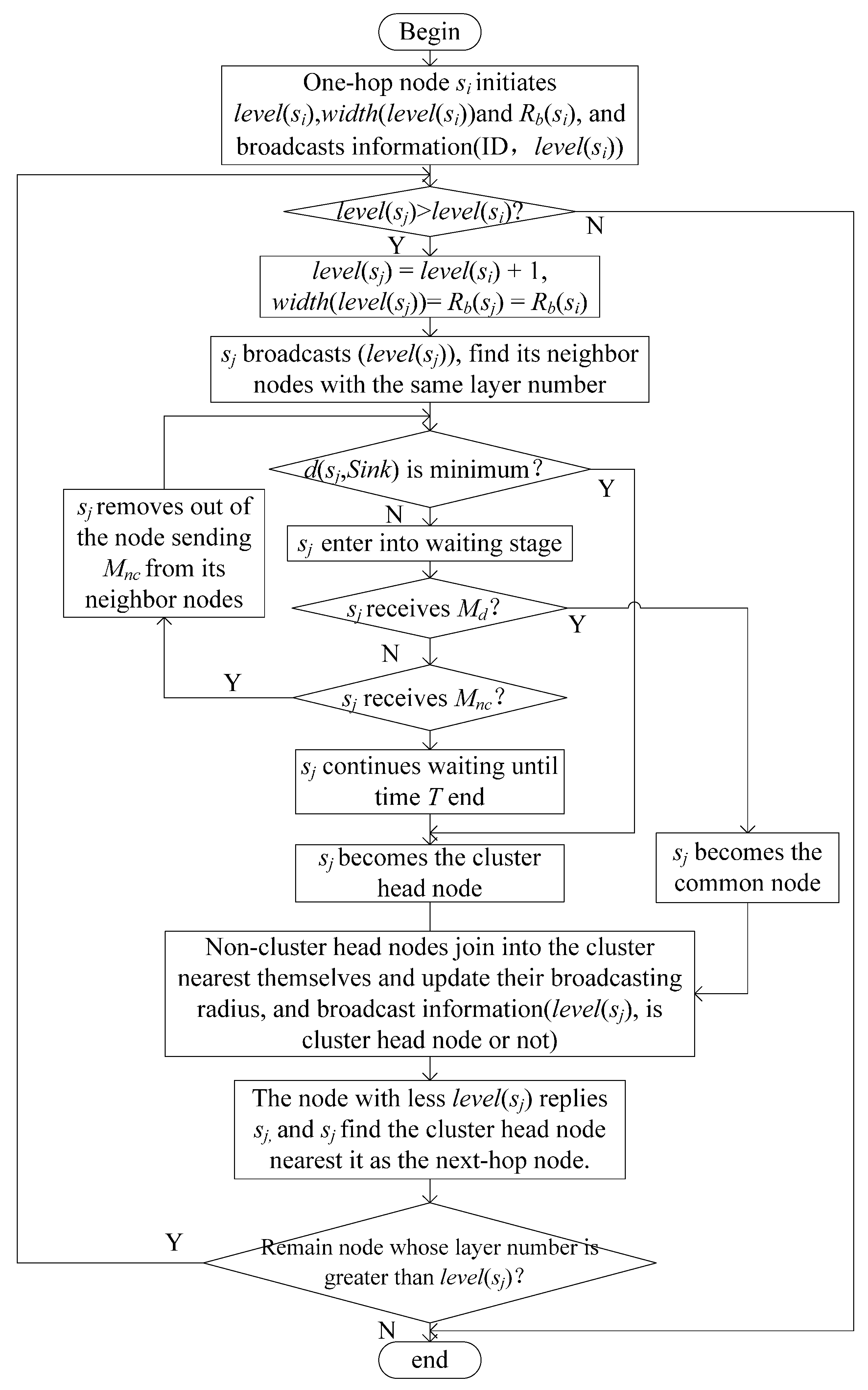
- After the one-hop node si moves to the calculated position, all the other one-hop nodes set their layer number, level(si), to 1; the corresponding layer width, width(level(si)), to the initial communication radius, ; and the broadcast radius, Rb(si), to . Then, they broadcast their information, (ID, level(si)).
- Step 2.
- The node sj receiving the information compares the layer number with that of si. If the layer number is greater than that of si, then level(sj) is set to level(si) + 1 and Rb(sj), and width(level(sj)) are set to Rb(si).
- Step 3.
- The node sj broadcasts the information level(sj), and the nodes having the same layer number as sj reply the distance between the sink node and themselves to sj. Then, sj compares the distance with its distance to the sink node, d(sj,Sink), to determine if d(sj,Sink) is the minimum value among the distances of the nodes relaying the distance to sj. Consequently, sj becomes a cluster head node and broadcasts the information Mc. By contrast, sj enters the stage of waiting message. In time T, if sj receives Mc, then sj becomes a common node and broadcasts Mnc. If sj receives Mnc, then sj ignores the distance a node sent and compares its distance to the sink node with that of the nodes, except the node sending Mnc. sj also becomes the cluster head node when sj waits for time T. The common node then joins into the cluster, which is the closest to it, and the nodes in current layer update the broadcast radius Rb(sj),
- Step 4.
- Each node sj in the current layer broadcasts the information (level(sj), cluster head node or not). For the node receiving the information, the node whose layer number is greater than level(sj) proceeds to Step 2 and clusters with the residual nodes. The node whose layer number is less than level(sj), relays the information (self is cluster head node or not) to the cluster head node and ignores the information the common nodes send. The cluster head node in the current layer selects the closest cluster head node in the last layer as the next-hop node. If it does not receive the information of the cluster head node in the last layer, then it selects the closest common node in the last layer as the next-hop node.
After a certain time, if the node has the initial layer number, then it broadcasts its maximum communication radius and enters the closest cluster. If the node has the initial layer number and only has neighbor nodes with the initial layer number in its maximum communication radius, then this node moves a distance in the direction of the sink node one time and subsequently finds its next-hop node. Distance (signed as dsink in following paper) here refers to the average distance between the node and its closest node in the direction of the sink node minus the maximum communication radius.
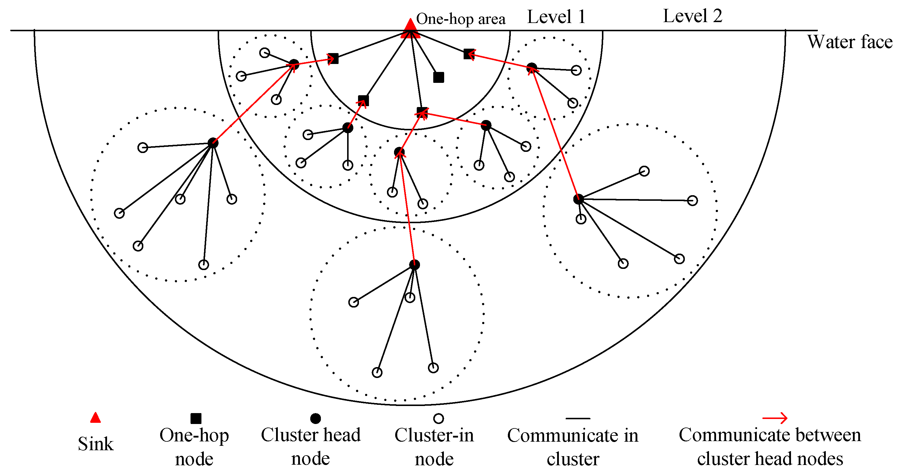
After Stage (2) is run, the network distribution is generally shown in Figure 3. The number of the cluster in the region near the sink node is greater than that in the region far from the sink node.
The flowchart of network layering and clustering is presented in Figure 4.
(3) Optimizing the Position of the Cluster-in Nodes
After Stage (2), each cluster node (i.e., sk) knows its own cluster-in node set Sc(sk) and their corresponding original positions Po(sk). When the cluster head node, sk, receives the command “calculating deployment location”, it calculates the deployment position of its cluster-in nodes.
First, sk updates the set of nodes whose deployment positions have been calculated in the network SND and the set of nodes whose deployment positions have been calculated in its cluster SCD (the element in SCD is only the cluster head node when the cluster head node begins to optimize the positions of its cluster-in nodes). Subsequently, sk calculates the deployment positions of its cluster-in nodes by using PSOA, and the deployment position of each cluster-in node is determined using PSOA once. The detailed procedure follows.
(1) Selecting Next Node to be Calculated
The cluster head node sk calculates the CRR values of its cluster-in nodes whose deployment positions in the network have not yet been calculated and then selects the node (i.e., si) with the minimum CRR as the next node to be calculated.
(2) Constructing the Fitness Function
The cluster head node sk firstly formulizes the deployment energy consumption that nodes move from the initial position to the deployment position and subsequently formulizes the increase in the network coverage. Finally, sk regards the ratio of the deployment energy consumption to the increase in the network coverage as the fitness function fitness2 on the premise that si can connect with at least one node in SCD after si moves to the deployment position. The fitness functions fitness2 is formulated as follows:
where the numerator is the moving distance and the denominator is the network coverage gain when the node moves from the original position to the current deployed position.
The constraint conditions of this fitness function are as follows:
The node si connects with at least one node in SCD after it moves to the deployment position:
where
The deployment position of si is in the target area:
(3) Solving the Fitness Function by PSOA
For the selection of the optimal deployment position of a cluster-in node, the pigeon swarm is initialized on the basis of the fitness function and solution space. A description of pigeon swarm initialization follows.
Rule for initializing the pigeon swarm: Each pigeon represents a possible deployment position of the current calculating node, namely, the coordinates of the position in the target area. Thus, the initial position of each pigeon j can be expressed as Xj = [x,y,z]. The solution space of the deployment location may consist of multiple intersecting spheres. Thus, the same amount of pigeons is produced in every sphere because pigeons search for the solution space thoroughly to obtain the optimal solution as much as possible. On the assumption that |SCD| nodes whose deployment positions have been calculated in the cluster of sk, the rule for producing the initial population is as follows: Np/|SCD| random points (i.e., the position of the pigeon) are produced in each sphere, with each node in SCD as its center and 1.25 as its radius; all the random points form the initial population of the pigeon. The initial speed of the pigeon is derived randomly in the interval 0−Vmax.
The steps to derive the optimal solution by PSOA are as follows:
- (1)
- The pigeons are initialized. The Np initial positions of the pigeons are determined using the rule for initializing the pigeon swarm.
- (2)
- The fitness of each individual is calculated. The fitness values are sorted according to the following rule: the fitness values of the individuals beyond the solution space are less than those in the solution space. The individual with the minimum fitness is selected as the global optimal solution, Xg, in the current iteration. When several individuals have the same minimum fitness, the individual with the minimum distance to the sink node is selected as Xg.
- (3)
- The position of the pigeon is updated using Equations (8) and (9), the fitness value is calculated, and Xg is updated according to Step (2).
- (4)
- If the value of the current iteration is not equal to the maximum number of iterations, N1, then Step (3) is repeated.
- (5)
- The solution space based on Equations (10)–(12) is searched locally, and Xg is updated.
- (6)
- If the number of iterations is not N2, then Step (5) is repeated.
- (7)
- Xg is the deployment location of node si.
When sk has calculated the deployment positions of its cluster-in nodes, each node moves to the corresponding position and broadcasts its new position. The other nodes whose deployment positions are not calculated update their SND.
The cluster head node sk inquires its last-hop node (sk’s child node) whether the deployment positions of its cluster-in nodes have been calculated. If not, the last-hop node of sk begins to calculate the deployment positions of its cluster-in nodes according to Stage (3) “Optimizing the Position of the Cluster-in Nodes” in Section 4.2.2. Otherwise, sk transmits the information that the deployment positions of the node in its cluster have been calculated to its next-hop node (sk’s father node), and its next-hop node finds the next cluster where the deployment positions of cluster-in nodes need to be calculated, following the procedure described above in the current paragraph. When all of the clusters in the network have completed the process “Optimizing the Position of the Cluster-in Nodes”, the algorithm ends.
The following Algorithm 1 provides the main steps of the process of optimizing the position of the cluster-in nodes.
| Algorithm 1. Optimizing the Position of the Cluster-in Nodes. | ||
| Input: set of cluster-in nodes Sc(sk), original position of the cluster-in nodes Po(sk). Output: deployed position of the cluster-in node Pd(sk). 1: Initialize Pd(sk) = zeros(|Sc(sk)|, 3), SND, SCD = sk; 2: while Sc(sk) 3: calculate the CRR of the node in Sc(sk); 4: si = the node with the minimum CRR; 5: poriginal(si) = [xoriginal, yoriginal, zoriginal] according to Po(sk); 6: assuming that pdeployed(si) = [xdeployed,ydeployed,zdeployed] and build the fitness function; 7: initialize N1, N2, Np, G, and the search range; 8: initialize the position Xj and the speed Vj of each pigeon individual j; 9: calculate the fitness2 of each pigeon individual; 10: Xg = arg min[fitness2(Xj)]; 11: for Nt = 1 to N1 do 12: for i = 1 to Np do 13: calculate Vi and Xi according to Equations (8) and (9); 14: end for 15: evaluate Xi, and update Xg; 16: end for 17: for Nt = 1 to N2 do 18: if Np > 1 19: rank the fitness2; 20: Np = Np/2; 21: removed the half of pigeons with a lower fitness2; 22: calculate Xc according to Equation (11); 23: for i = 1 to Np do (remaining pigeons) 24: calculate Vi and Xi according to Equation (12); 25: end 26: evaluate Xi, and update Xg; 27: end if 28: end for 29: record Xg into Pd(sk), namely, update the value of corresponding row in Pd(sk); 30: Sc(sk) = Sc(sk) − si; 31: SND = SND si; 32: SCD = SCD si; 33: end while; | ||
| Notice: Po(sk) and Pd(sk) are the matrix with the size |Sc(sk)| × 3, and Po(sk) = [Poriginal(s1); Poriginal(s2);⋯, Poriginal(si)]. In addition, zeros(|Sc(sk)|, 3) is the matrix whose element is zero and whose size is size |Sc(sk)| × 3. | ||
5. Algorithm Analysis
This section analyzes the time complexity of the algorithm. The relevant parameters are presented in Table 1.
5.1. Time Complexity of PSOA
PSOA comprises the map and compass operator model and the landmark operator model. During the map and compass operator, each pigeon updates its position according to the global optimal solution, Xg, produced in the last iteration, and subsequently Xg is updated in each of the iterations. The execution time of each of the iterations is 2Np. Thus, the model’s time complexity, complexity1, is 2(N1Np).
In each of the iterations during the landmark operator, the algorithm initially sorts the pigeons according to their fitness values to calculate the center position, Xc. The execution time of this process is Np log Np. The algorithm then updates the position of each pigeon according to Xc and updates Xg; the execution time of this process is 2Np. Thus, the execution time of each of the iterations is NplogNp + 2Np, and the model’s time complexity, complexity2, is formulated as follows:
The time complexity of PSOA (complexityPSOA) is
5.2. Time Complexity of PSA
At the stage of network layering and clustering, the nodes broadcast layer by layer for network layering, and the number of layers is not better than size/. In each layer, the nodes select the cluster head node synchronously. The worst situation in this process is that a node waits for all its neighbor nodes to give up the competition one by one. The time complexity is Na. Thus, this stage’s time complexity, complexity3, is Na·size/.
At the stage of optimizing the positions of the cluster-in nodes, for each cluster, the algorithm firstly selects the node one by one to calculate their CRR, and then calculates the deployment location of each cluster-in node by using the PSOA iteratively, that is, the algorithm uses PSOA to calculate the deployment positions of cluster-in nodes one by one. Thus, for each cluster, the time complexity is Nci (complexityPSOA + Nci). Assuming that network has Nc cluster head nodes, this stage’s time complexity complexity4 is formulated as follow:
Therefore, the time complexity of PSA, complexityPSA, is formulated as follows:
6. Simulation and Performance Analysis
6.1. Simulation Scenario and Parameter Settings
This study simulates the node self-deployment process of an underwater wireless sensor network by using the MATLAB simulation platform to analyze the effectiveness of PSA. The target water area (length × width × depth) is set to 120 × 120 × 120 m3, the node sensing radius, Rs, is set to 10 m, and the result of each index is calculated as the average value of 30 sets of data. The other parameters are set as follows:
- (1)
- With the method of obtaining the optimal hot spot radius in [34] as basis, the minimum communication radius in this study is set to 12.5 m. The maximum communication radius is set to thrice that of Rs to be consistent with the simulation conditions of TVFDA.
- (2)
- The parameter G is set to 0.2, Vmax is set to 0.15 times that of the length of the target area, N1, N2 is respectively set to 35 and 30, and Np is set to 55 after several experiments on solving the fitness function. (The process is not described in detail in this paper because the experiment is not the point of the problem studied in the paper).
- (3)
- According to [35], the distance between the node and the boundary is 0.866Rs when the full coverage of the network is achieved. This distance is adopted in this study; that is, cboarder is set to 0.866Rs.
- (4)
- The parameter of the communication energy consumption model and other parameters are set as shown in Table 2.
6.2. Simulation
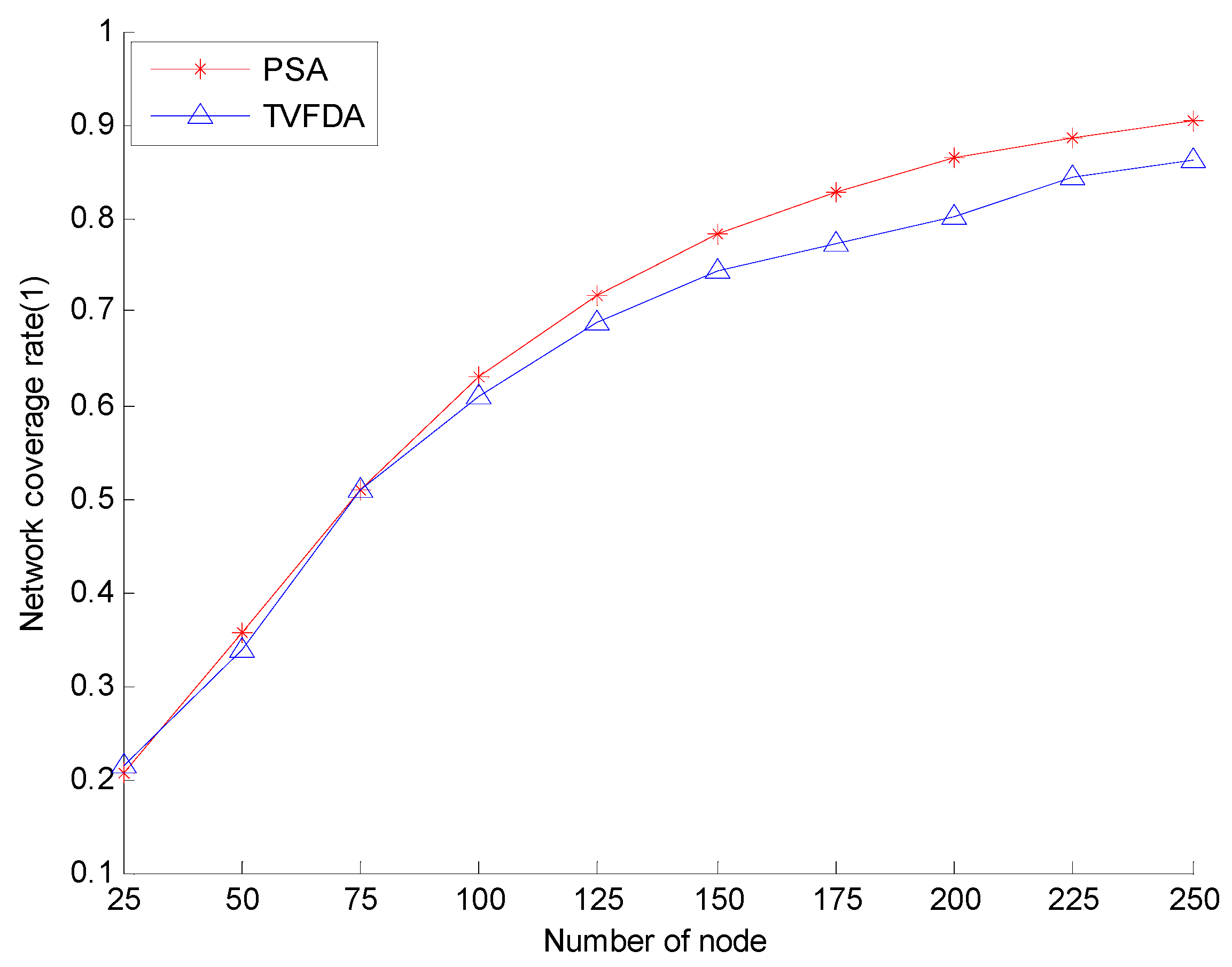
Figure 5 shows the network coverage rates of PSA and TVFDA with varying number of nodes. The coverage rates of PSA and TVFDA increase with increasing number of nodes. The coverage rates of PSA and TVFDA are highly similar when the number of nodes is lower than 75, but the coverage rate of PSA is higher than that of TVFDA. When the number of nodes is increased, PSA finds more optimal node deployment locations than TVFDA does. This result may be attributed to the process of PSA of determining the moving directions and distances of the nodes by building the optimization model and solving it using PSOA. When the number of the nodes is extremely low, the difference in the results between the two algorithms is not evident. Therefore, when the goal is to improve network reliability and network connectivity even at the risk of reducing network coverage, PSA can still provide network coverage that is slightly higher than TVFDA.
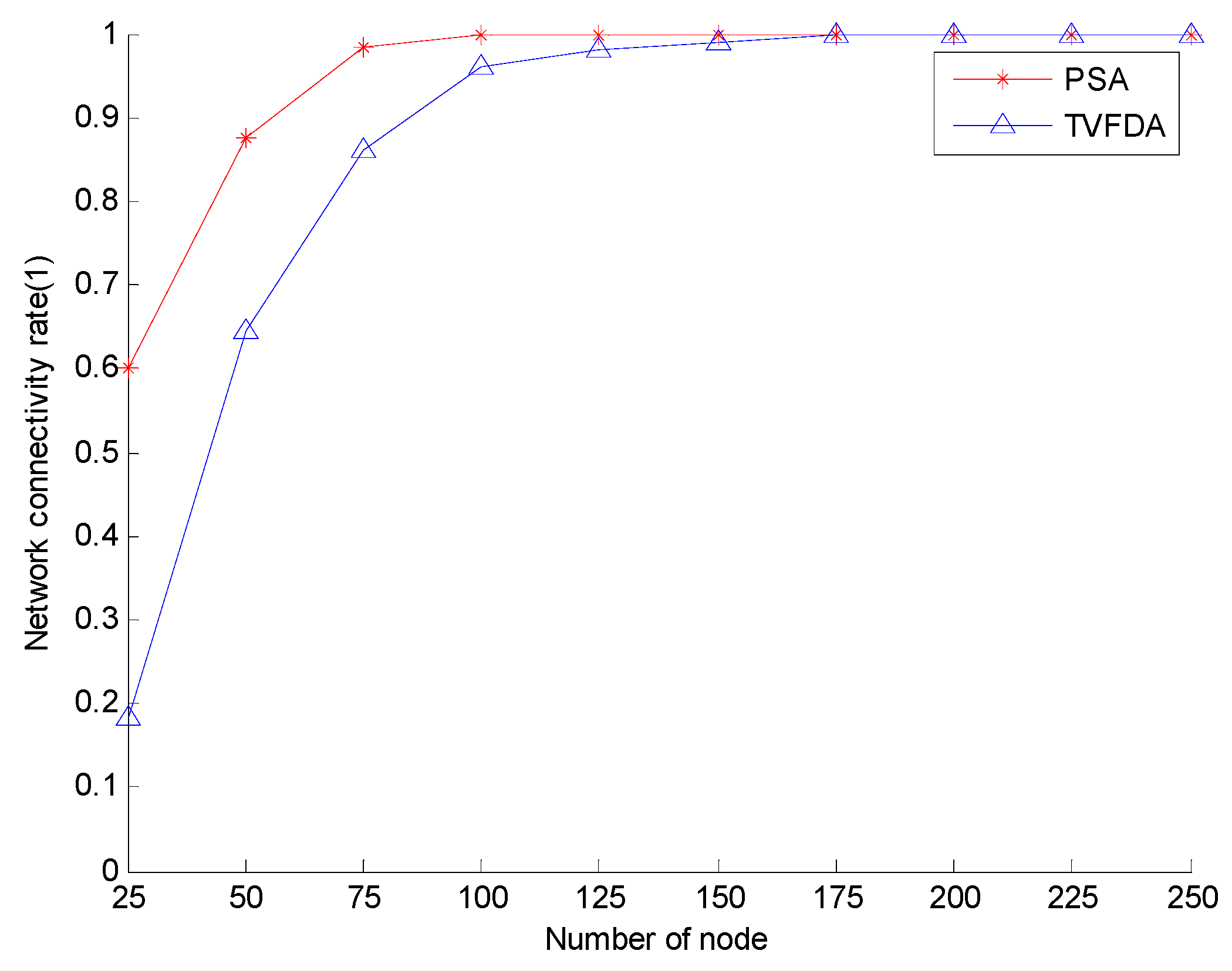
Figure 6 shows the network connectivity coefficients of PSA and TVFDA with varying number of nodes. The network connectivity coefficients of PSA and TVFDA increase with increasing number of nodes, and PSA can even reach the state of full network connectivity. Moreover, the network connectivity of PSA is higher than TVFDA when the network nodes are sparse. The superiority of PSA can be attributed to the process of optimizing the node positions by first constructing the backbone of the network and subsequently optimizing the positions of the cluster-in nodes on the condition of maintaining network connectivity. When the network nodes are sparse, all the nodes cannot constitute the backbone network, and the unconnected nodes randomly move a certain distance in the direction of the sink node, thereby increasing network connectivity to a certain extent. By contrast, TVFDA determines the moving direction and distance of each node according to the neighbor of the node, which is very easy to cause the original connected network to be divided and consequently reducing the connectivity of the entire network.
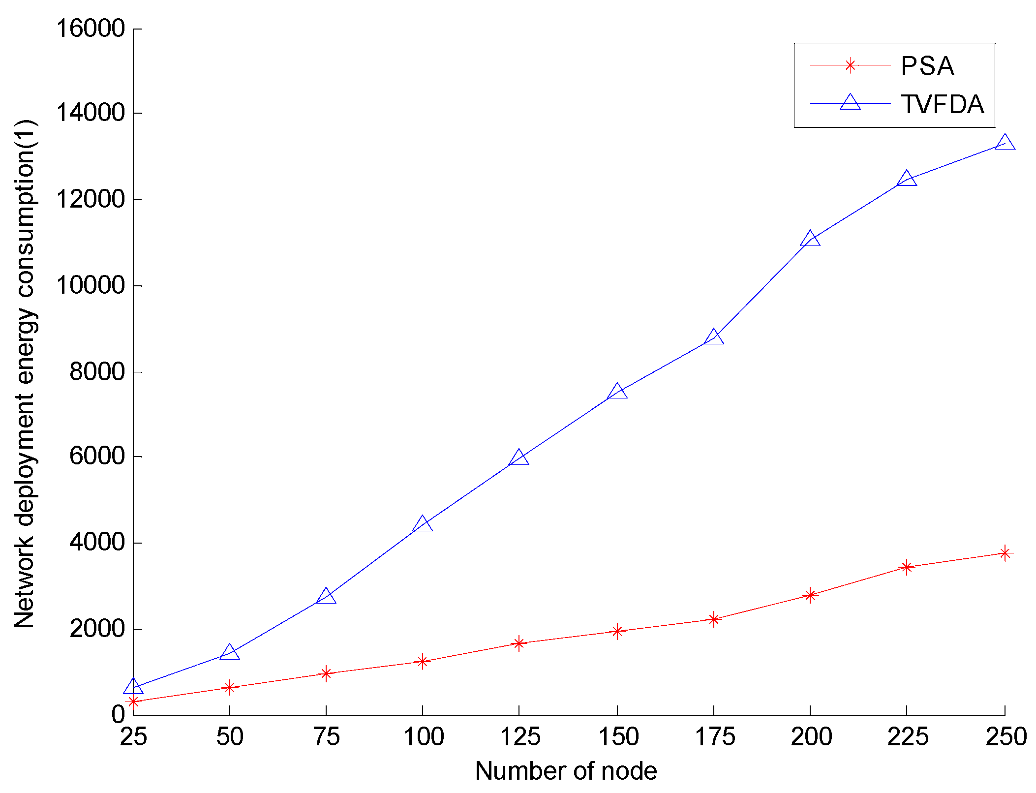
Figure 7 shows the network deployment energy consumption of PSA and TVFDA with varying number of nodes. As shown, the network deployment energy consumption of both algorithms increase with increasing number of nodes, but the network deployment energy consumption growth of TVFDA is significantly greater than that of PSA. In TVFDA, almost all the nodes in the algorithm have to move corresponding distances several times according to the virtual forces exerted on them; thus, the total distance of the node during the network deployment process significantly increases. In PSA, the nodes only move once during the execution of the algorithm, and the network deployment energy consumption is considered when calculating the deployment locations of the cluster-in nodes. In addition, when the network nodes are sparse, a node has no neighbors with large probability, that is, some nodes may not move when TVFDA runs, thereby reducing the total moving distance to a certain extent. Thus, the deployment energy consumption of TVFDA is approximate to PSA when the number of nodes is low.
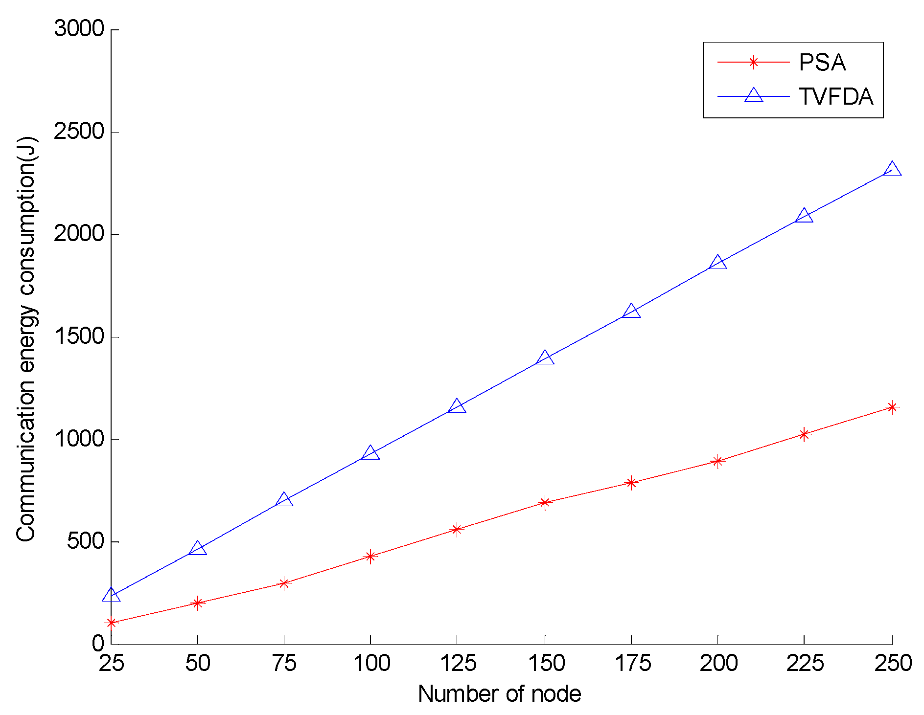
Figure 8 shows the communication energy consumption of PSA and TVFDA with varying number of nodes. As shown, the communication energy consumption of PSA is lower than that of TVFDA. TVFDA needs to run several iterations in a distributed manner to improve the network coverage and connectivity, and each node in each of the iterations needs to broadcast a message to obtain the environment information. (According to many experiments, TVFDA needs to run approximately 15 times before stabilizing, when the communication radius of the nodes is 30 m and the nodes are deployed in an area of 120 × 120 × 120 m3). However, at the network layering and clustering stage of PSA, each node needs to broadcast a maximum of four messages, and the communication radii of all the nodes are less than the maximum communication radius. Moreover, the locations of the nodes in the cluster can be obtained by optimizing the node position, that is, each of cluster-in nodes should broadcast once. Therefore, PSA is better than TVFDA in terms of communication energy consumption.
Figure 9 shows the number of nodes in the region within the distance to the sink node with varying number of nodes in the entire network. As shown, the numbers of nodes in both algorithms increase. However, for the same number of nodes, the number of nodes in the sink node area after PSA deployment is greater than that after TVFDA deployment. PSA does not optimize the cluster head nodes in the entire network and the number of the cluster head node is greater in the region near the sink node, which increases the number of nodes in the region. However, the objective of TVFDA is to promote the uniform distribution of nodes in the network to increase the coverage of the network without considering the number of nodes in the vicinity of the sink node.
7. Conclusions
In this study, we propose PSA for UWSNs to solve the problem in which existing free-to-move node self-deployment algorithms usually target event coverage and cannot improve network coverage under the premise of considering network connectivity, network reliability and network deployment energy consumption. In this algorithm, the sink node first finds its one-hop nodes and maximizes the network coverage in its one-hop region. The one-hop nodes then divide the network into layers and cluster in each layer. Meanwhile, each cluster head node constructs a connected path to the sink node to guarantee network connectivity. The cluster head node finally regards the ratio of the movement distance of the node to the change in CRR as the target function. It employs pigeon swarm optimization to solve the node-deployment problem. The simulation results show that PSA improves both network connectivity and network reliability, decreases network deployment energy consumption, and increases the network coverage.
As a future work, we plan to extend the ideas in this paper considering the node deployment about node probability perception model, which is more in line with the actual situation. The cluster-in position adjustment strategy may need to be modified to some degree. In addition, we plan to consider the additional scenario where the sensor nodes are not anchored. In the scenario, the node may be drifted by the current, and the algorithm should run several times to maximize the network service quality. Thus, the additional trigger mechanism that makes the algorithm run again will be designed.
Acknowledgments
This paper was supported by The National Key Research and Development Program of China (2016YFC0201400); The Provincial Key Research and Development Program of Science and Technology Department of Zhejiang Province (2016C03G2040707); The National Natural Science Foundation of China (NSFC61273072); and the National Natural Science Foundation of China and Zhejiang Joint Fund for Integrating of Informatization and Industrialization (U1509217).
Author Contributions
Shanen Yu, Yiming Xu and Peng Jiang conceived and designed the research; Shanen Yu, Yiming Xu and Peng Jiang performed the research; and Shanen Yu, Yiming Xu, Peng Jiang, Feng Wu, and Huan Xu wrote the paper.
Conflicts of Interest
The authors declare no conflict of interest.
References
- Yick, J.; Mukherjee, B.; Ghosal, D. Wireless sensor network survey. Comput. Netw. 2008, 52, 2292–2330. [Google Scholar] [CrossRef]
- Han, G.; Zhang, C.; Shu, L.; Sun, N.; Li, Q. A survey on deployment algorithms in underwater acoustic sensor networks. Int. J. Distrib. Sens. Netw. 2013, 9, 1–11. [Google Scholar] [CrossRef]
- Guo, Z.W.; Luo, H.J.; Hong, F.; Yang, M.; Lionel, M.N. Current Progress and Research Issues in Underwater Sensor Networks. J. Comput. Res. Dev. 2010, 47, 377–389. [Google Scholar]
- Heidemann, J.; Stojanovic, M.; Zorzi, M. Underwater sensor networks: Applications, advances and challenges. Phil. Trans. R. Soc. A 2012, 370, 158–175. [Google Scholar] [CrossRef] [PubMed]
- Lloret, J. Underwater sensor nodes and networks. Sensors 2013, 13, 11782–11796. [Google Scholar] [CrossRef] [PubMed]
- Climent, S.; Capella, J.V.; Meratnia, N.; Serrano, J.J. Underwater Sensor Networks: A New Energy Efficient and Robust Architecture. Sensors 2012, 12, 704–731. [Google Scholar] [CrossRef] [PubMed]
- Han, G.; Jiang, J.; Shu, L.; Xu, Y.; Wang, F. Localization Algorithms of Underwater Wireless Sensor Networks: A Survey. Sensors 2012, 12, 2026–2061. [Google Scholar] [CrossRef] [PubMed]
- Han, G.; Zhang, C.; Shu, L. Impacts of Deployment Strategies on Localization Performance in Underwater Acoustic Sensor Networks. IEEE Trans. Ind. Electron. 2015, 62, 1725–1733. [Google Scholar] [CrossRef]
- Verma, D.; Tripathi, A.K. Time Synchronization in Wireless Sensor Network Based on Level Discovery Phase. Int. J. Comput. Appl. 2014, 104, 101–111. [Google Scholar]
- Yoon, S.; Azad, A.K.; Oh, H.; Kim, S. AURP: An AUV-Aided Underwater Routing Protocol for Underwater Acoustic Sensor Networks. Sensors 2012, 12, 1827–1845. [Google Scholar] [CrossRef] [PubMed]
- Wu, H.; Chen, M.; Guan, X. A Network Coding Based Routing Protocol for Underwater Sensor Networks. Sensors 2012, 12, 4559–4577. [Google Scholar] [CrossRef] [PubMed]
- Aziz, A.A.; Sekercioglu, Y.A.; Fitzpatrick, P.; Ivanovich, M. A Survey on Distributed Topology Control Techniques for Extending the Lifetime of Battery Powered Wireless Sensor Networks. IEEE Commun. Surv. Tutor. 2013, 15, 121–144. [Google Scholar] [CrossRef]
- Alam, S.M.; Haas, Z.J. Coverage and Connectivity in Three-Dimensional Networks. In Proceedings of the 12th annual international conference on Mobile computing and networking, Los Angeles, CA, USA, 24–29 September 2006; ACM: New York, NY, USA, 2006; pp. 346–357. [Google Scholar]
- Felamban, M.; Shihada, B.; Jamshaid, K. Optimal Node Placement in Underwater Wireless Sensor Networks. In Proceedings of the IEEE 27th International Conference on Advanced Information Networking and Applications (AINA), Barcelona, Spain, 25–28 March 2013; pp. 492–499. [Google Scholar]
- Detweiler, C.; Doniec, M.; Vasilescu, I. Autonomous Depth Adjustment for Underwater Sensor Networks: Design and Applications. IEEE/ASME Trans. Mechatron. 2012, 17, 16–24. [Google Scholar] [CrossRef]
- Senel, F.; Akkaya, K.; Erol-Kantarci, M.; Yilmaz, T. Self-deployment of mobile underwater acoustic sensor networks for maximized coverage and guaranteed connectivity. Ad Hoc Netw. 2014, 34, 170–183. [Google Scholar] [CrossRef]
- Akkaya, K.; Newell, A. Self-deployment of sensors for maximized coverage in underwater acoustic sensor networks. Comput. Commun. 2009, 32, 1233–1244. [Google Scholar] [CrossRef]
- Cayirci, E.; Tezcan, H.; Dogan, Y.; Coskun, V. Wireless sensor networks for underwater survelliance systems. Ad Hoc Netw. 2006, 4, 431–446. [Google Scholar] [CrossRef]
- Ibrahim, S.; Liu, J.; Al-Bzoor, M.; Cui, J.H.; Ammar, R. Towards efficient dynamic surface gateway deployment for underwater network. Ad Hoc Netw. 2013, 11, 2301–2312. [Google Scholar] [CrossRef]
- Wang, G.; Cao, G.; La, P.T.F. Movement-assisted sensor deployment. IEEE Trans. Mob. Comput. 2006, 5, 640–652. [Google Scholar] [CrossRef]
- Wang, G.; Cao, G.; La, P.T. Sensor Relocation in Mobile Sensor Networks. In Proceedings of the IEEE 24th Annual Joint Conference of the IEEE Computer and Communications Societies, Miami, FL, USA, 13–17 March 2005; Volume 4, pp. 2302–2312. [Google Scholar]
- Koutsougeras, C.; Liu, Y.; Zheng, R. Event-driven sensor deployment using self-organizing maps. Int. J. Sens. Netw. 2008, 3, 142–151. [Google Scholar] [CrossRef]
- Xia, N.; Wang, C.S.; Zheng, R.; Jiang, J.G. Fish Swarm Inspired Underwater Sensor Deployment. ACTA Autom. Sin. 2012, 38, 295–302. [Google Scholar] [CrossRef]
- Du, H.; Xia, N.; Zheng, R. Particle Swarm Inspired Underwater Sensor Self-Deployment. Sensors 2014, 14, 15262–15281. [Google Scholar] [CrossRef] [PubMed]
- Li, X.Y.; Ci, L.L.; Yang, M.H. Deploying Three-Dimensional Mobile Sensor Networks Based on Virtual Forces Algorithm; Springer: Berlin/Heidelberg, Germany, 2013; pp. 204–216. [Google Scholar]
- Xu, X.; Ansari, R.; KhoKhar, A. Hierarchical data aggregation using compressive sensing (HDACS) in WSNs. ACM Trans. Sens. Netw. (TOSN) 2015, 11, 45–55. [Google Scholar] [CrossRef]
- Tsai, Y.R. Coverage-preserving routing protocols for randomly distributed wireless sensor networks. IEEE Trans. Wirel. Commun. 2007, 6, 1240–1245. [Google Scholar] [CrossRef]
- Garcia, M.; Sendra, S.; Atenas, M.; Lloret, J. Underwater Wireless Ad-Hoc Networks: A Survey. In Mobile Ad Hoc Networks: Current Status and Future Trends; CRC Press: Boca Raton, FL, USA, 2011; pp. 379–411. [Google Scholar]
- Ahmed, S.; Javaid, N.; Khan, F.A. Co-UWSN: Cooperative Energy-Efficient Protocol for Underwater WSNs. Int. J. Distrib. Sens. Netw. 2015, 11, 891410. [Google Scholar] [CrossRef] [PubMed]
- Duan, H.; Luo, Q. New progresses in swarm intelligence–based computation. Int. J. Bio-Inspired Comput. 2015, 7, 26–35. [Google Scholar] [CrossRef]
- Duan, H.; Qiao, P. Pigeon-inspired optimization: A new swarm intelligence optimizer for air robot path planning. Int. J. Intell. Comput. Cybern. 2014, 7, 24–37. [Google Scholar] [CrossRef]
- Li, C.; Duan, H. Target detection approach for UAVs via improved pigeon-inspired optimization and edge potential function. Aerosp. Sci. Technol. 2014, 39, 352–360. [Google Scholar] [CrossRef]
- Dou, R.; Duan, H. Pigeon inspired optimization approach to model prediction control for unmanned air vehicles. Aircr. Eng. Aerosp. Technol. Int. J. 2016, 88, 108–116. [Google Scholar] [CrossRef]
- Ye, M.; Chan, E.; Chen, G. On Mitigating Hot Spots for Clustering Mechanisms in Wireless Sensor Networks. In Proceedings of the IEEE International Conference on Mobile Adhoc and Sensor Systems (MASS), Vancouver, BC, Canada, 9–12 October 2006; pp. 558–561. [Google Scholar]
- Laranjeira, L.A.; Rodrigues, G.N. Border effect analysis for reliability assurance and continuous connectivity of wireless sensor networks in the presence of sensor failures. IEEE Trans. Wirel. Commun. 2014, 13, 4232–4246. [Google Scholar] [CrossRef]
Figure 1.
Underwater 3D space model.

Figure 2.
Solution coding diagram.

Figure 3.
Network Distribution Diagram.

Figure 4.
Flowchart of network layering and clustering.

Figure 5.
Network coverage comparison.

Figure 6.
Network connectivity comparison.

Figure 7.
Network deployment energy consumption comparison.

Figure 8.
Network communication energy consumption comparison.

Figure 9.
Network reliability comparison.


Table 1.
Symbol Table.
| Parameters | Symbol |
|---|---|
| Target area size | size |
| Population number | Np |
| Iteration number of the map and compass operator model | N1 |
| Iteration number of the landmark model | N2 |
| Average number of neighbor | Na |
| Average number of non-cluster head node | Nci |
| Minimum communication radius |
Table 2.
Parameter setting.
| Parameter | Value |
|---|---|
| Length of data packet Lb | 150 bit |
| Carrier frequency Fr | 24 kHZ |
| Energy consumption of data reception Pr | 20 mW |
| Data transmission speed underwater Vt | 1000 bit/s |
© 2017 by the authors. Licensee MDPI, Basel, Switzerland. This article is an open access article distributed under the terms and conditions of the Creative Commons Attribution (CC BY) license (http://creativecommons.org/licenses/by/4.0/).
Share and Cite
MDPI and ACS Style
Yu, S.; Xu, Y.; Jiang, P.; Wu, F.; Xu, H. Node Self-Deployment Algorithm Based on Pigeon Swarm Optimization for Underwater Wireless Sensor Networks. Sensors 2017, 17, 674. https://doi.org/10.3390/s17040674
AMA Style
Yu S, Xu Y, Jiang P, Wu F, Xu H. Node Self-Deployment Algorithm Based on Pigeon Swarm Optimization for Underwater Wireless Sensor Networks. Sensors. 2017; 17(4):674. https://doi.org/10.3390/s17040674
Chicago/Turabian StyleYu, Shanen, Yiming Xu, Peng Jiang, Feng Wu, and Huan Xu. 2017. "Node Self-Deployment Algorithm Based on Pigeon Swarm Optimization for Underwater Wireless Sensor Networks" Sensors 17, no. 4: 674. https://doi.org/10.3390/s17040674
Note that from the first issue of 2016, this journal uses article numbers instead of page numbers. See further details here.