Comparative Evaluation of Background Subtraction Algorithms in Remote Scene Videos Captured by MWIR Sensors


Abstract
1. Introduction
1.1. Motivation and Contribution
- (1)
- The released BS datasets [2,3,4,5] do not focus on the remote scene. Background subtraction and moving targets detection in remote scene video is important and common to lots of fields, such as battlefield monitoring, intrusion detection and outdoor remote surveillance. Remote scene IR video sequences present typical characteristics: small and even dim foreground, less color, texture and gradient information in the foreground (FG) and background (BG), which causes difficulty for BS and affects the performance of BS. It is necessary to develop a remote scene IR dataset and evaluate BS algorithms on it.
- (2)
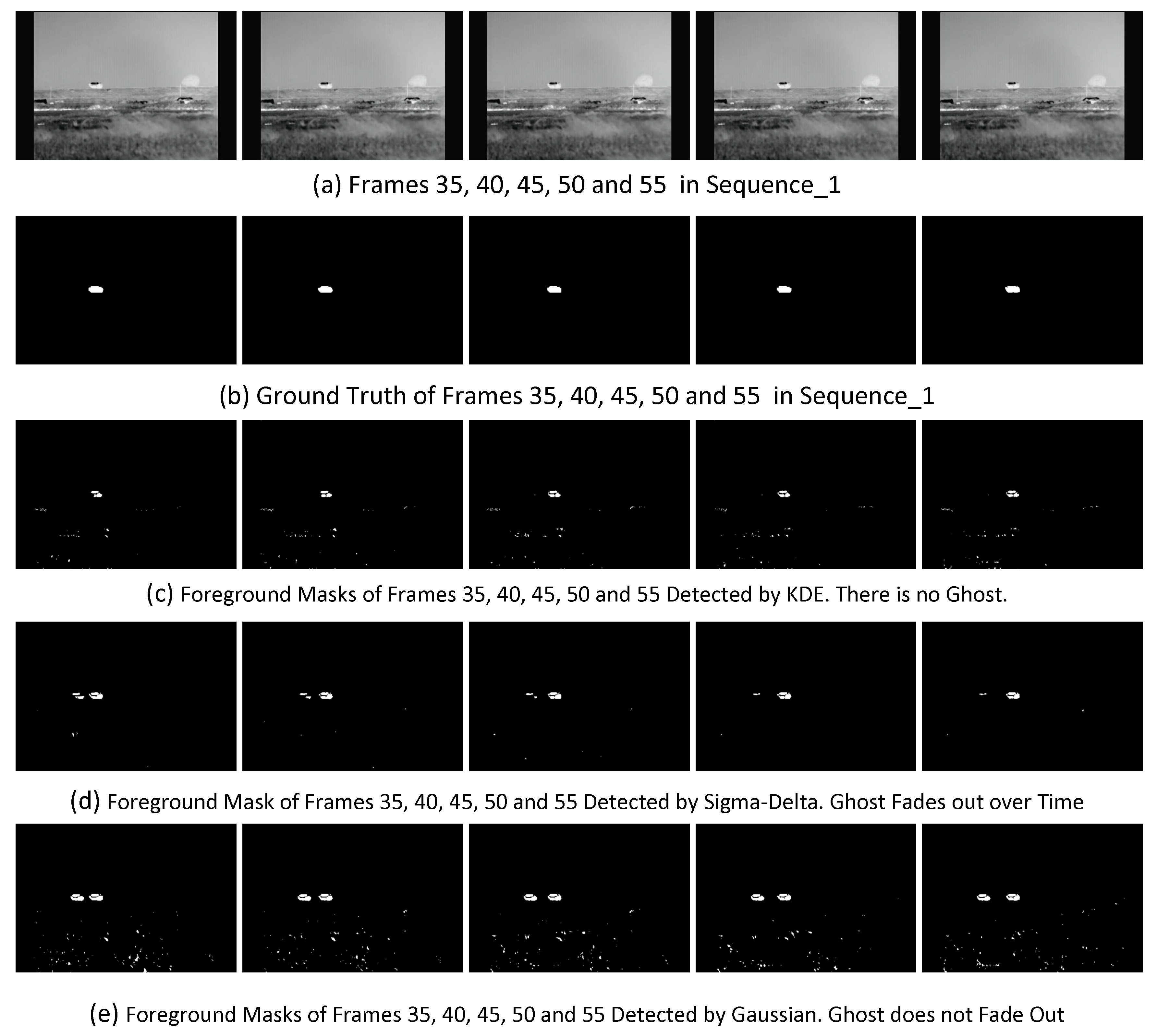
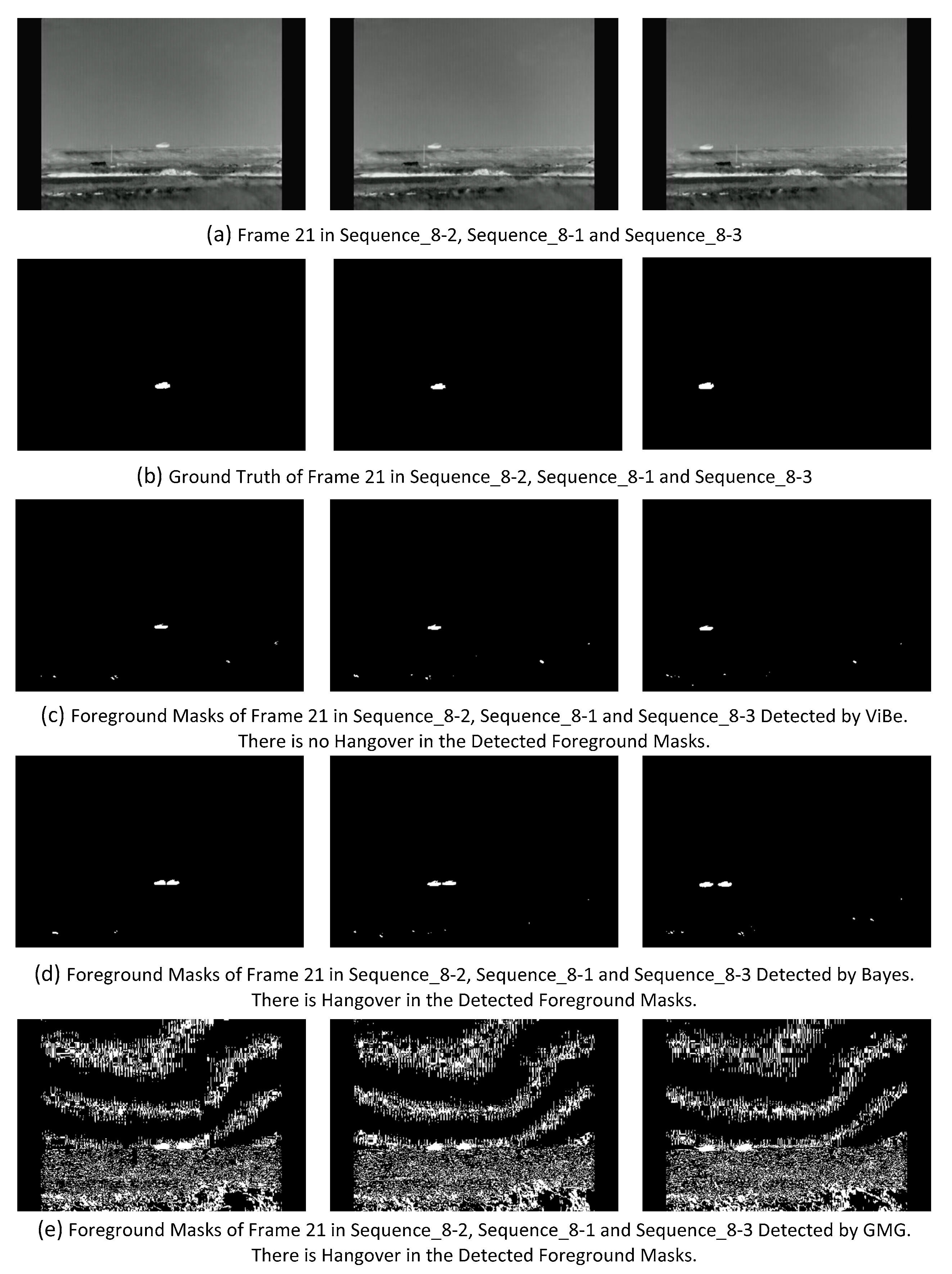
- The challenges of high and low speeds of foreground movement have been identified in previous works [6,7], and are presented in the released cVSG dataset [6]. For the challenge of high speed of foreground movement, if the speed is high enough, such as beyond 1 self-size per frame, which means that there is no overlap between the foregrounds in two sequential frames, some BS algorithms would yield hangover as shown in Figure 14. In the BS paradigm, each pixel is labeled as foreground or background. For the challenge of low speed of foreground movement, if the speed is low enough, especially below 1 pixel per frame, it is much more difficult to distinguish the foreground pixels. It is important to evaluate BS algorithms to cope with these two challenges. The speed units self-size/frame and pixel/frame are adopted respectively for the high and low speed challenges in this evaluation paper.
- (3)
- In the published evaluation papers, there is not enough experimental data and analysis on some identified BS challenges. Camouflage is an identified challenge [3,4,8,9] which is caused by foreground that has similar color and texture as the background, but these papers do not provide a video sequence representing it. Reference [2] provided a synthetic video sequence representing camouflage challenges concerning color. Camouflaged foreground is unavoidable in video surveillance. It is important to conduct evaluation experiments on real video sequences representing this challenge.
- (4)
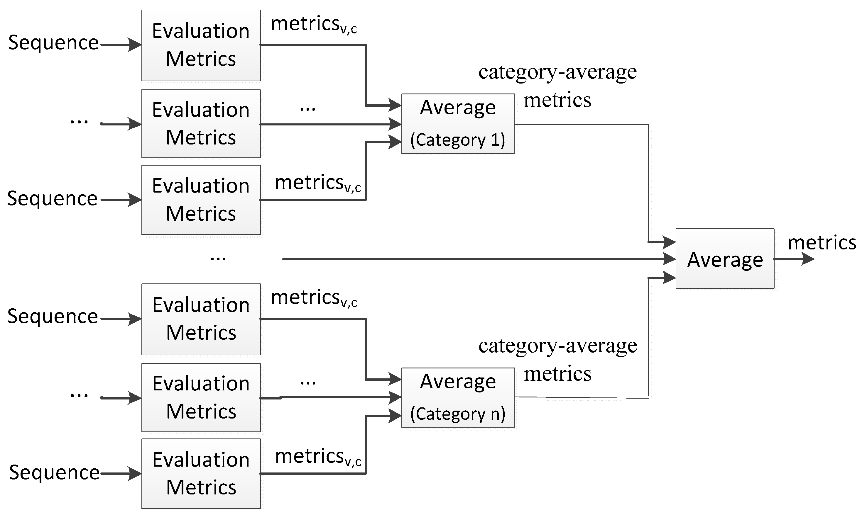
- It is illogical to evaluate the capability of BS to handle kinds of challenges based on the whole video sequence or category with same evaluation metrics. Previous works [2,3,4] always group the video sequences into several categories according to the type of challenge, and evaluate the capability of BS algorithms to handle these challenges with same evaluation metrics based on the whole category. Actually some challenges such as camera jitter only last for several frames or impact several frames. Some challenges such as shadow and ghosting only occupy small parts of the frame. To evaluate the capability of BS to handle these challenges, it is logical to evaluate the performance change caused by these challenges with proper evaluation metrics or criteria. As examples, for camera jitter, we should focus on the frames after it occurs and the changes of performance; for ghosting, we should focus on whether it appears and how many frames it lasts for; for high speed of foreground movement, we should focus on whether the hangover phenomenon appears and how many frames the hangover lasts for.
- (5)
- There is no detailed implementation and parameter setting in some BS algorithm papers [10,11] and previous evaluation papers [5,8,12]. Because of the different implementations, the same BS algorithm often performs differently. It is reasonable to detail the implementation and parameter setting of the evaluated BS algorithms.
- (6)
- The comparison is not fair in some previous evaluation experiments. Post-processing is a common way to improve the performance of BS. BS algorithms [13,14,15,16,17] utilize and benefit from post-processing as part of the BS process. It would be fairer to remove post-processing from these BS algorithms and evaluate the BS algorithms without and with post-processing, respectively.
- (1)
- A remote scene IR BS dataset captured by our designed MWIR sensor is provided with identified challenges and pixel-wise ground truth of foreground.
- (2)
- BS algorithms are summarized in six important issues which are used to describe the implementation of BS algorithms. The implementations of the evaluated BS algorithms are detailed according to these issues. The parameter settings are also presented in this paper.
- (3)
- (4)
- BS algorithm evaluation experiments were conducted on the proposed remote scene IR dataset. The overall performance of the evaluated BS algorithms and processor/memory requirements are compared. Proper evaluation metrics and criteria are selected to evaluate the capability of BS to handle the identified BS challenges represented in the proposed dataset.
1.2. Organization of This Paper
2. Previous Works
2.1. Previous Datasets
2.2. Previous Evaluation and Review Papers
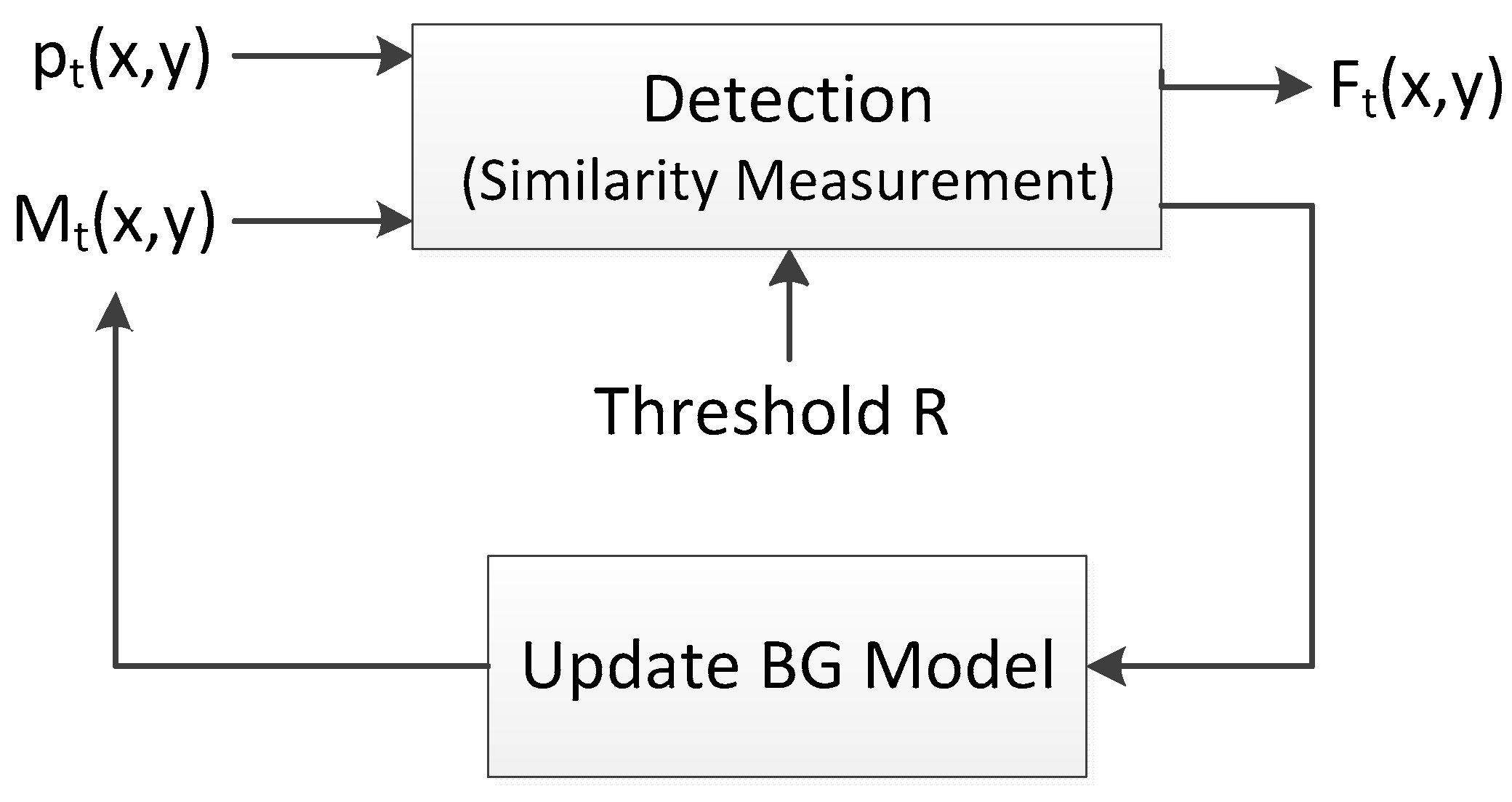
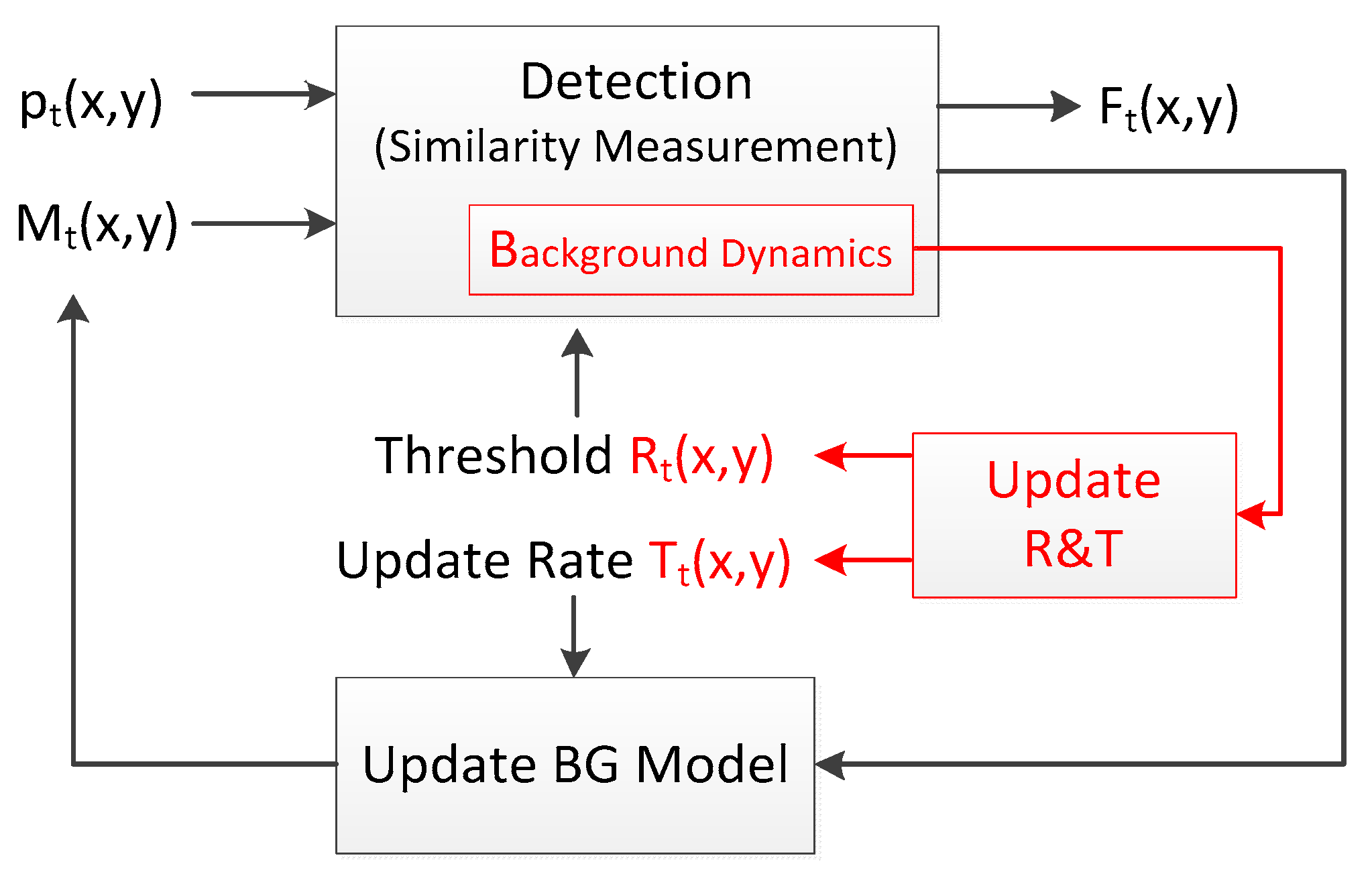
3. Overview of Background Subtraction
3.1. Description of Background Subtraction Algorithm
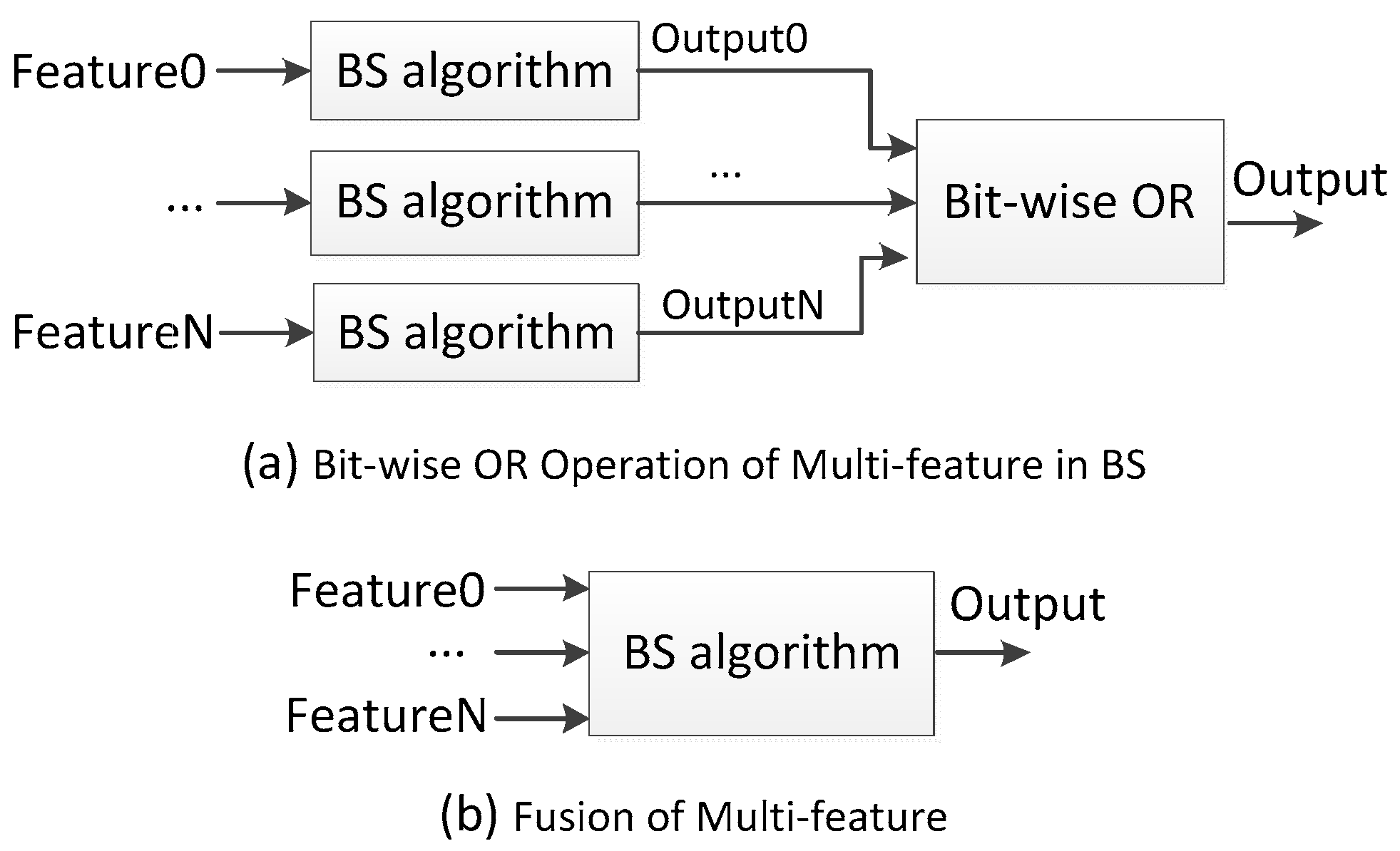
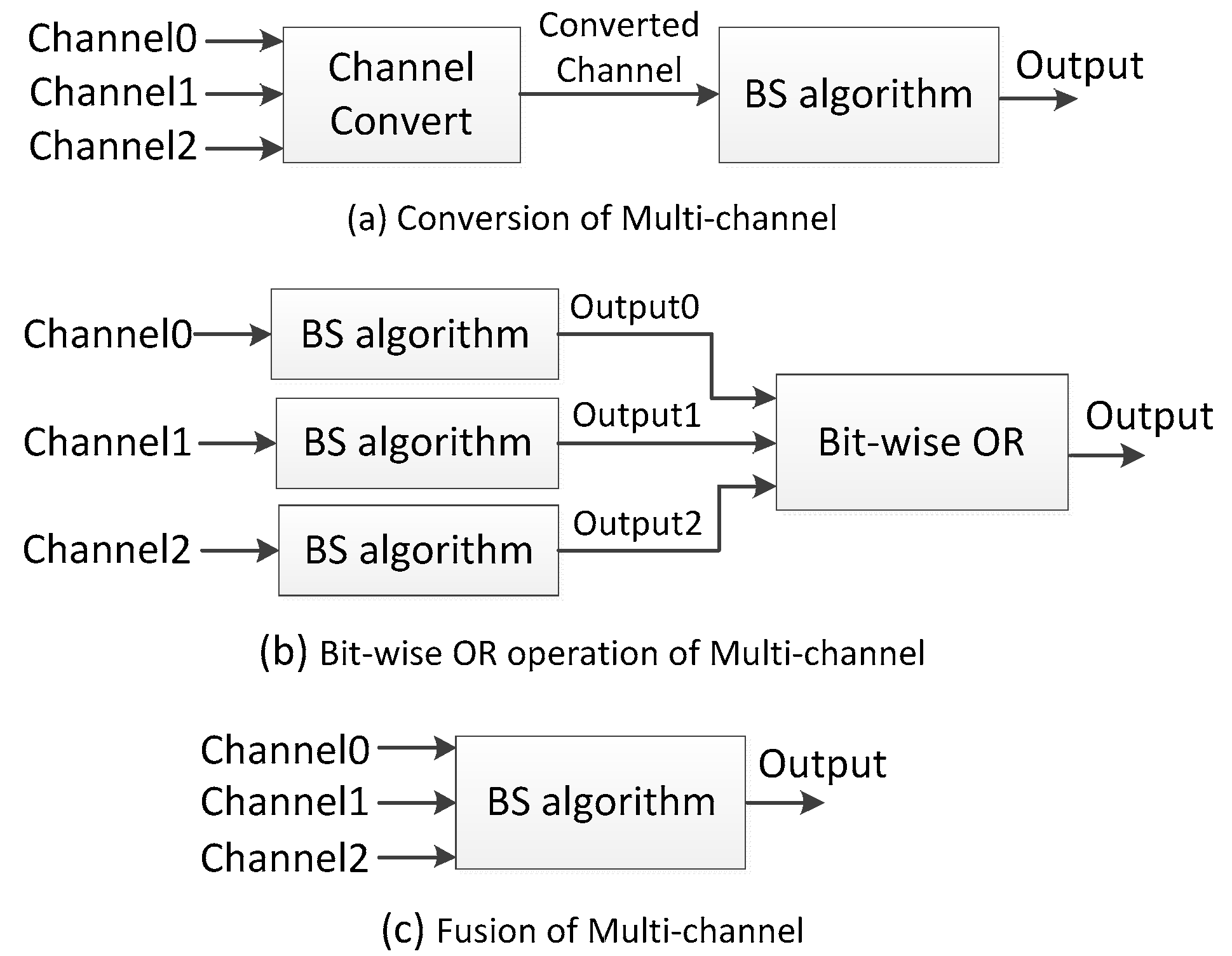
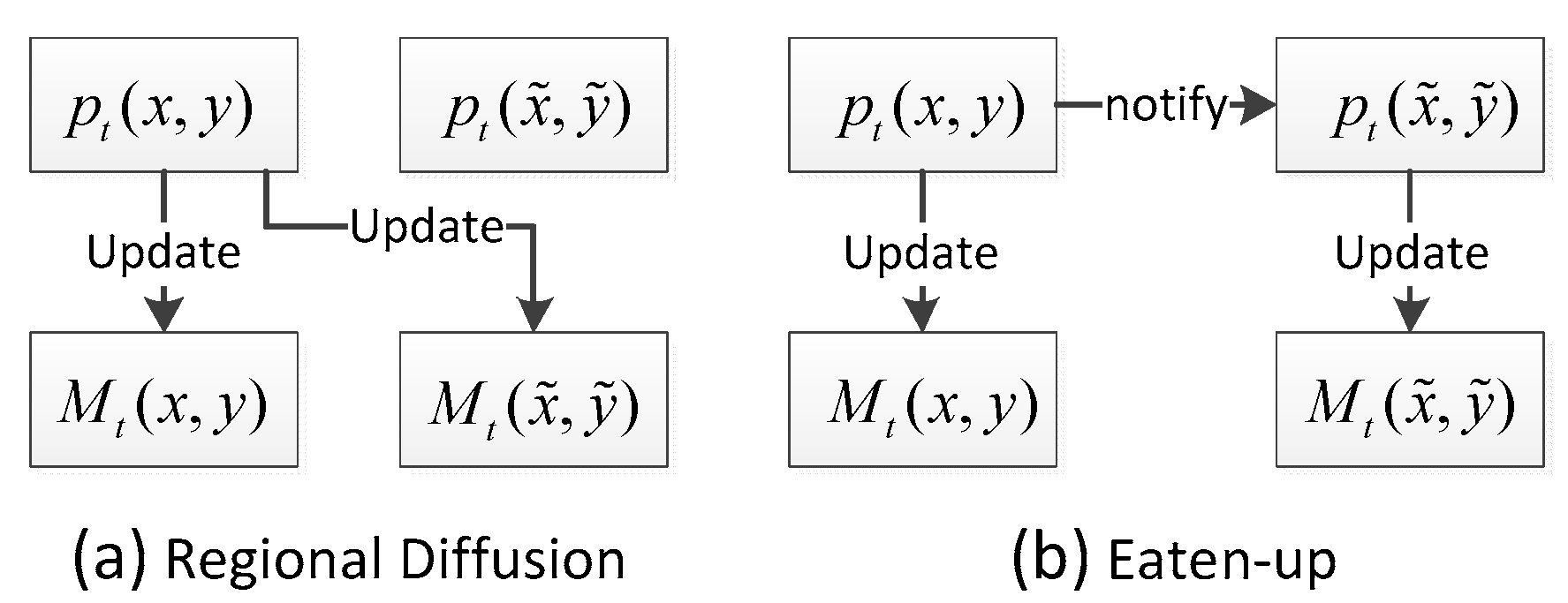
3.2. New Mechanisms in BS Algorithm
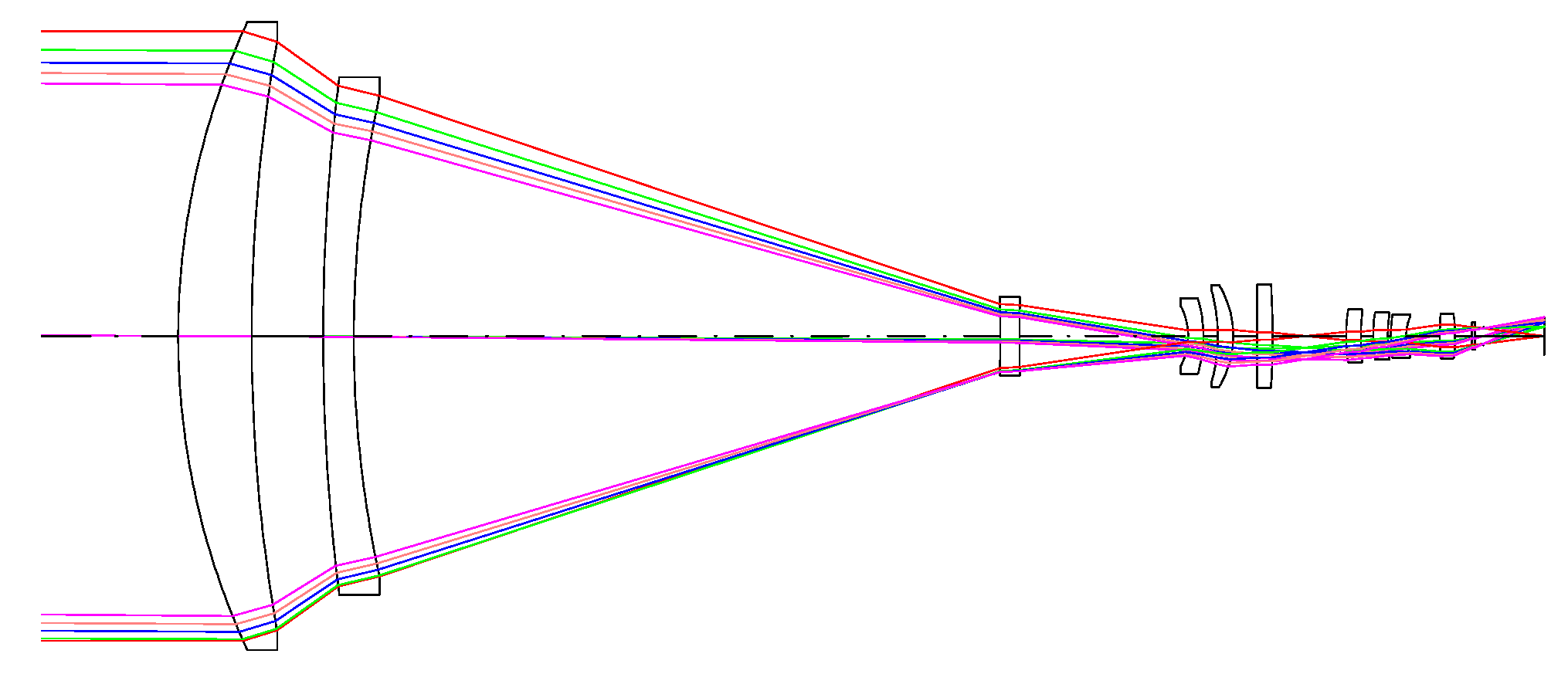
4. MWIR Sensor and Remote Scene IR Dataset
5. Experimental Setup
5.1. Implementation of BS Algorithms
5.2. Parameter Settings of BS Algorithms
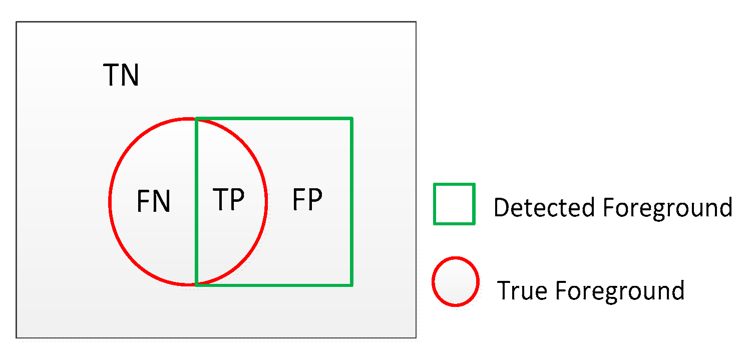
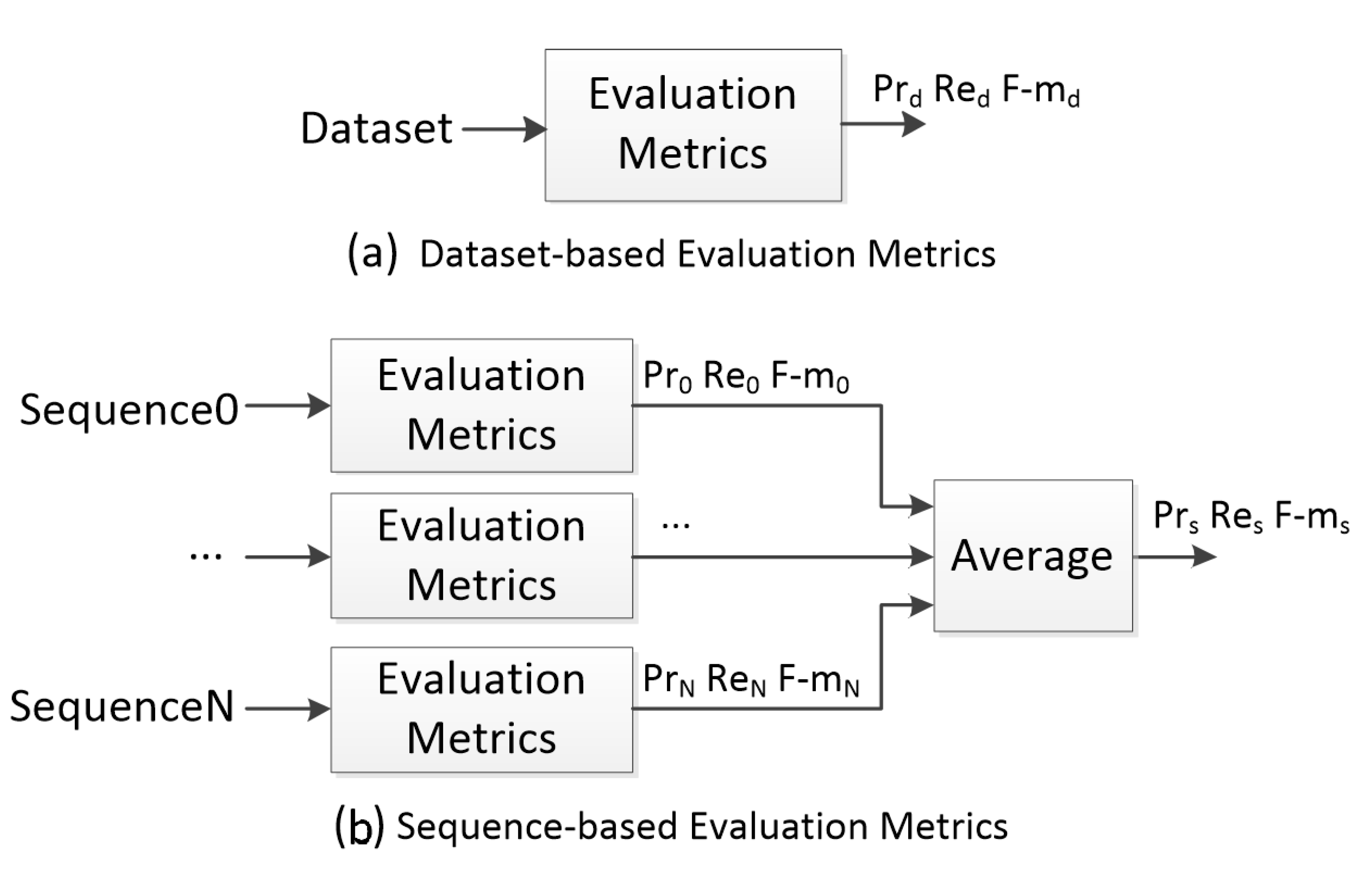
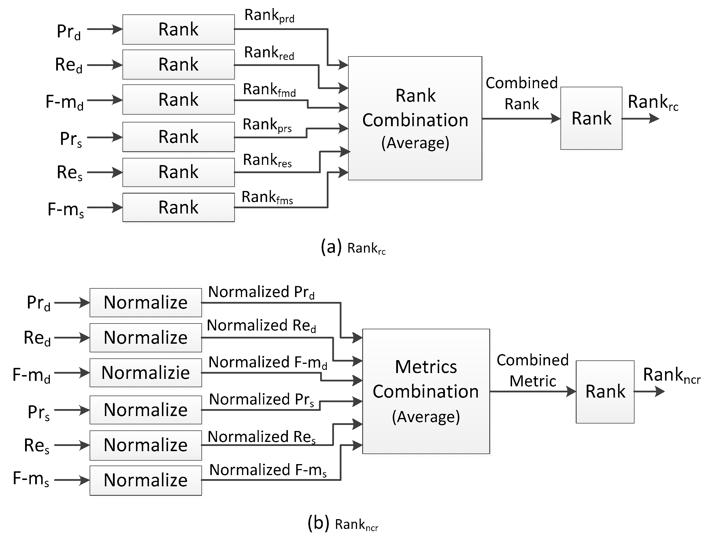
5.3. Statistical Evaluation Metrics
5.4. Rank-Order Rules
5.5. Other Evaluation Metrics
6. Experimental Results
6.1. Overall Results
6.2. Post-Processing
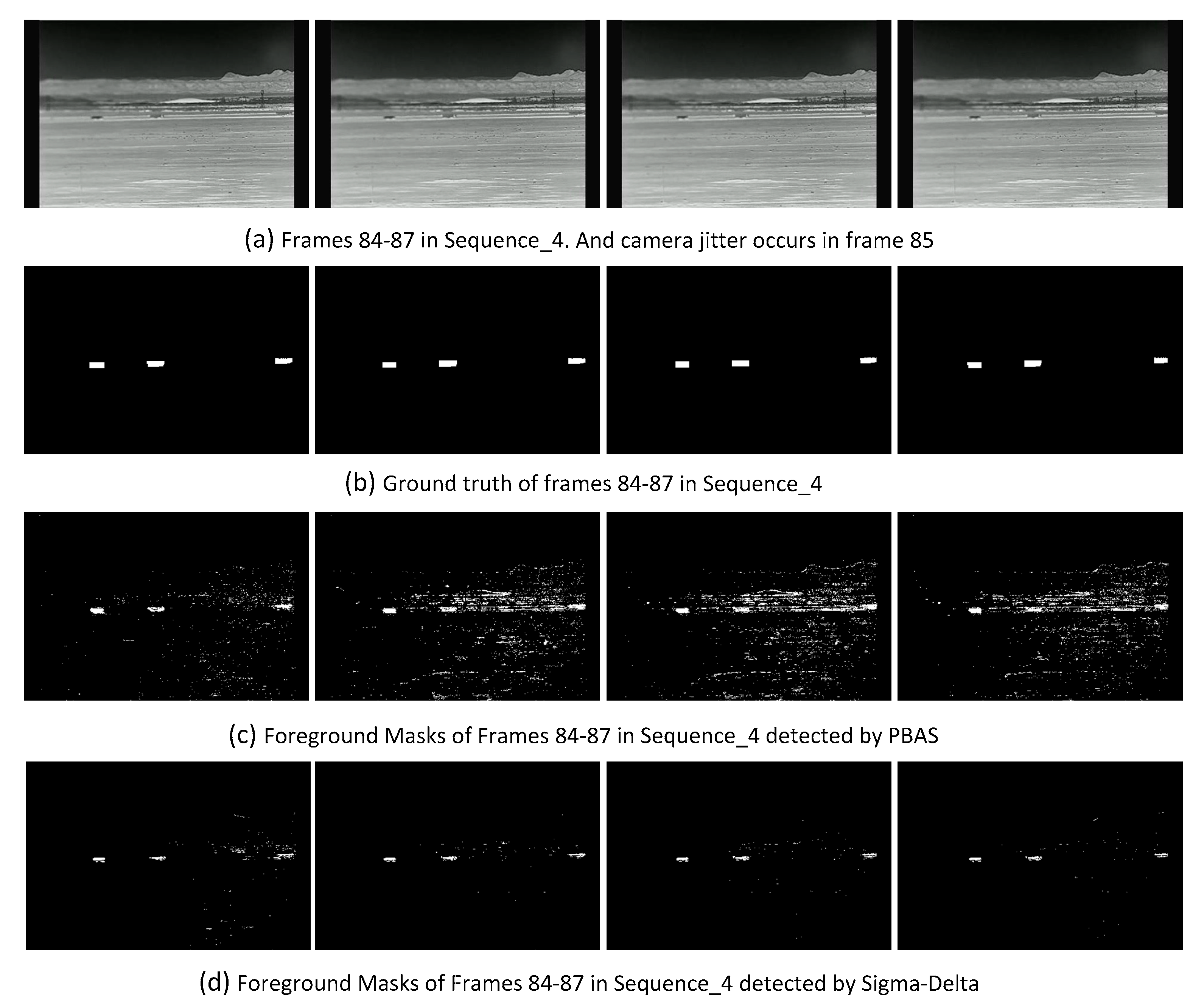
6.3. Camera Jitter
6.4. Ghosts
6.5. Low Speed of Foreground Movement
6.6. High Speed of Foreground Movement
6.7. Camouflage
6.8. Small Dim Foreground
6.9. Computational Load and Memory Usage
6.10. Extensional Evaluation with BGSLibrary
7. Discussion
Supplementary Materials
Acknowledgments
Author Contributions
Conflicts of Interest
References
- Sobral, A. BGSLibrary: An OpenCV C++ Background Subtraction Library. In Proceedings of the 2013 IX Workshop de Viso Computacional. Rio de Janeiro, Brazil, 3–5 January 2013. [Google Scholar]
- Brutzer, S.; Hoferlin, B.; Heidemann, G. Evaluation of Background Subtraction Techniques for Video Surveillance. In Proceedings of the 24th IEEE Conference on Computer Vision and Pattern Recognition, Colorado Springs, CO, USA, 20–25 June 2011; pp. 1937–1944. [Google Scholar]
- Goyette, N.; Jodoin, P.; Porikli, F.; Konrad, J. Changedetection.net: A New Change Detection Benchmark Dataset. In Proceedings of the 25th IEEE Conference on Computer Vision and Pattern Recognition, Providence, RI, USA, 16–21 June 2012; pp. 1–8. [Google Scholar]
- Wang, Y.; Jodoin, P.; Porikli, F.; Konrad, J.; Benezeth, Y.; Ishwar, P. CDnet 2014: An Expanded Change Detection Benchmark Dataset. In Proceedings of the 27th IEEE Conference on Computer Vision and Pattern Recognition, Columbus, OH, USA, 24–27 June 2014; pp. 393–400. [Google Scholar]
- Vacavant, A.; Chateau, T.; Wilhelm, A.; Lequievre, L. A Benchmark Dataset for Outdoor Foreground/Background Extraction. In Proceedings of the 11th Asian Conference on Computer Vision, Daejeon, Korea, 5–9 November 2012; pp. 291–300. [Google Scholar]
- Tiburzi, F.; Escudero, M.; Bescos, J.; Martínez, J. A Ground-truth for Motion-based Video-object Segmentation. In Proceedings of the 2008 IEEE International Conference on Image Processing, San Diego, CA, USA, 12–15 October 2008; pp. 17–20. [Google Scholar]
- Shaikh, S.; Saeed, K.; Chaki, N. Moving Object Detection Approaches, Challenges and Object Tracking. In Moving Object Detection Using Background Subtraction, 1st ed.; Springer International Publishing: New York, NY, USA, 2014; pp. 5–14. [Google Scholar]
- Benezeth, Y.; Jodoin, P.; Emile, B.; Laurent, H.; Rosenberger, C. Comparative study of background subtraction algorithms. J. Electron. Imaging 2010, 19, 033003. [Google Scholar]
- Bouwmans, T. Traditional and recent approaches in background modeling for foreground detection: An overview. Comput. Sci. Rev. 2014, 11, 31–66. [Google Scholar] [CrossRef]
- McFarlane, N.; Schofield, C. Segmentation and tracking of piglets in images. Mach. Vis. Appl. 1995, 8, 187–193. [Google Scholar] [CrossRef]
- Wren, R.C.; Azarbayejani, A.; Darrell, T.; Pentland, P.A. Pfinder: Real-time tracking of the human body. IEEE Trans. Pattern Anal. Mach. Intell. 1997, 19, 780–785. [Google Scholar] [CrossRef]
- Dhome, Y.; Tronson, N.; Vacavant, A.; Chateau, T.; Gabard, C.; Goyat, Y.; Gruyer, D. A Benchmark for Background Subtraction Algorithms in Monocular Vision: A Comparative Study. In Proceedings of the 2nd International Conference on Image Processing Theory Tools and Applications, Melbourne, Australia, 15–17 April 2010; pp. 66–71. [Google Scholar]
- Godbehere, A.; Matsukawa, A.; Goldberg, K. Visual Tracking of Human Visitors under Variable-Lighting Conditions for a Responsive Audio Art Installation. In Proceedings of the 2012 American Control Conference, Montreal, QC, Canada, 27–29 June 2012; pp. 4305–4312. [Google Scholar]
- Zivkovic, Z.; Heijiden, F. Efficient adaptive density estimation per image pixel for the task of background subtraction. Pattern Recognit. Lett. 2006, 27, 773–780. [Google Scholar] [CrossRef]
- Zivkovic, Z. Improved Adaptive Gaussian Mixture Model for Background Subtraction. In Proceedings of the 17th International Conference on Pattern Recognition, Cambridge, UK, 23–26 August 2004; pp. 28–31. [Google Scholar]
- Li, L.; Huang, W.; Gu, I.; Tian, Q. Foreground Object Detection from Videos Containing Complex Background. In Proceedings of the 11th ACM International Conference on Multimedia, Berkeley, CA, USA, 4–6 November 2003; pp. 2–10. [Google Scholar]
- Maddalena, L.; Petrosino, A. A self-organizing approach to background subtraction for visual surveillance applications. IEEE Trans. Image Process. 2008, 17, 1168–1177. [Google Scholar] [CrossRef] [PubMed]
- Brown, L.; Senior, A.; Tian, Y.; Vonnel, J.; Hampapur, A.; Shu, C.; Merkl, H.; Lu, M. Performance Evaluation of Surveillance Systems under Varying Conditions. In Proceedings of the 7th IEEE International Workshop on Performance Evaluation of Tracking and Surveillance, Breckenridge, CO, USA, 7 January 2005; pp. 79–87. [Google Scholar]
- Toyama, K.; Krumm, J.; Brumiit, B.; Meyers, B. Wallflower: Principles and Practice of Background Maintenance. In Proceedings of the 7th IEEE International Conference on Computer Vision, Kerkyra, Greece, 20–27 September 1999; pp. 255–261. [Google Scholar]
- Piater, H.J.; Crowley, L.J. Multi-modal Tracking of Interacting Targets Using Gaussian Approximations. In Proceedings of the 2nd IEEE International Workshop on Performance Evaluation of Tracking and Surveillance, Kauai, HI, USA, 9 December 2001; pp. 141–177. [Google Scholar]
- Sheikh, Y.; Shah, M. Bayesian modeling of dynamic scenes for object detection. IEEE Trans. Pattern Anal. Mach. Intell. 2005, 27, 1778–1792. [Google Scholar] [CrossRef] [PubMed]
- Vezzani, R.; Cucchiara, R. Video surveillance online repository (ViSOR): An integrated framework. Multimed Tools Appl. 2010, 50, 359–380. [Google Scholar] [CrossRef]
- Bloisi, D.; Pennisi, A.; Locchi, L. Background modeling in the maritime domain. Mach. Vis. Appl. 2014, 25, 1257–1269. [Google Scholar] [CrossRef]
- Camplani, M.; Blanco, C.; Salgado, L.; Jaureguizar, F.; Garcia, N. Advanced background modeling with RGB-D sensors through classifiers combination and inter-frame foreground prediction. Mach. Vis. Appl. 2014, 25, 1197–1210. [Google Scholar] [CrossRef]
- Camplani, M.; Salgado, L. Background foreground segmentation with RGB-D kinect data: An efficient combination of classifiers. J. Vis. Commun. Image Represent. 2014, 25, 122–136. [Google Scholar] [CrossRef]
- Fernandez-Sanchez, E.; Diaz, J.; Ros, E. Background subtraction model based on color and depth cues. Mach. Vis. Appl. 2014, 25, 1211–1225. [Google Scholar] [CrossRef]
- Fernandez-Sanchez, E.; Diaz, J.; Ros, E. Background subtraction based on color and depth using active sensors. Sensors 2013, 13, 8895–8915. [Google Scholar] [CrossRef] [PubMed]
- Benezeth, Y.; Jodoin, P.; Emile, B.; Laurent, H. Review and Evaluation of Commonly-Implemented Background Subtraction Algorithms. In Proceedings of the 19th IEEE International Conference on Pattern Recognition, Tampa, FL, USA, 8–11 December 2008; pp. 1–4. [Google Scholar]
- Prati, A.; Mikic, I.; Trivedi, M.; Cucchiara, R. Detecting moving shadows: Algorithms and evaluation. IEEE Trans. Pattern Anal. Mach. Intell. 2003, 25, 918–923. [Google Scholar] [CrossRef]
- Herrero, S.; Bescós, J. Background Subtraction Techniques: Systematic Evaluation and Comparative Analysis. In Proceedings of the 11th International Conference on Advanced Concepts for Intelligent Vision Systems, Bordeaux, France, 28 September–2 October 2009; pp. 33–42. [Google Scholar]
- Parks, D.; Fels, S. Evaluation of Background Subtraction Algorithms with Post-processing. In Proceedings of the 5th IEEE International Conference on Advanced Video and Signal Based Surveillance, Santa Fe, NM, USA, 1–3 September 2008; pp. 192–199. [Google Scholar]
- Karaman, M.; Goldmann, L.; Yu, D.; Sikora, T. Comparison of Static Background Segmentation Methods. In Proceedings of the SPIE Visual Communications and Image Processing, Beijing, China, 12–15 July 2005; pp. 2140–2151. [Google Scholar]
- Nascimento, J.; Marques, J. Performance evaluation of object detection algorithms for video surveillance. IEEE Trans. Multimed. 2006, 8, 761–774. [Google Scholar] [CrossRef]
- Prati, A.; Cucchiara, R.; Mikic, I.; Trivedi, M. Analysis and Detection of Shadows in Video Streams: A Comparative Evaluation. In Proceedings of the IEEE Conference on Computer Vision and Pattern Recognition, Kauai, HI, USA, 8–14 December 2001; pp. 571–577. [Google Scholar]
- Rosin, P.; Ioannidis, E. Evaluation of global image thresholding for change detection. Pattern Recognit. Lett. 2003, 24, 2345–2356. [Google Scholar] [CrossRef]
- Bashir, F.; Porikli, F. Performance Evaluation of Object Detection and Tracking Systems. In Proceedings of the 9th IEEE International Workshop on Performance Evaluation of Tracking Surveillance, New York, NY, USA, 18 June 2006. [Google Scholar]
- Radke, R.; Andra, S.; Al-Kofahi, O.; Roysam, B. Image change detection algorithms: A systematic survey. IEEE Trans. Image Process. 2005, 14, 294–307. [Google Scholar] [CrossRef] [PubMed]
- Piccardi, M. Background Subtraction Techniques: A Review. In Proceedings of the IEEE International Conference on Systems, Man and Cybernetics, The Hague, The Netherlands, 10–13 October 2004; pp. 3099–3104. [Google Scholar]
- Cheung, S.; Kamath, C. Robust Techniques for Background Subtraction in Urban Traffic Video. In Proceedings of the SPIE Video Communications and Image Processing, San Jose, CA, USA, 18 January 2004; pp. 881–892. [Google Scholar]
- Bouwmans, T.; Baf, E.F.; Vachon, B. Background modeling using mixture of Gaussians for foreground detection-a survey. Recent Pat. Comput. Sci. 2008, 1, 219–237. [Google Scholar] [CrossRef]
- Bouwmans, T. Recent Advanced statistical background modeling for foreground detection: A systematic survey. Recent Pat. Comput. Sci. 2011, 4, 147–176. [Google Scholar]
- Sobral, A.; Vacavant, A. A comprehensive review of background subtraction algorithms evaluated with synthetic and real videos. Comput. Vis. Image Underst. 2014, 122, 4–21. [Google Scholar] [CrossRef]
- Gruyer, D.; Royere, C.; Du, N.; Michel, G.; Blosseville, M. SiVIC and RTMaps, Interconnected Platforms for the Conception and the Evaluation of Driving Assistance Systems. In Proceedings of the 13th World Congress and Exhibition on Intelligent Transport Systems and Services, London, UK, 8–12 October 2006. [Google Scholar]
- Bouwmans, T. Subspace learning for background modeling: A survey. Recent Pat. Comput. Sci. 2009, 2, 223–234. [Google Scholar] [CrossRef]
- Heikklä, M.; Pietikäinen, M. A texture-based method for modeling the background and detecting moving objects. IEEE Trans. Pattern Anal. Mach. Intell. 2006, 28, 657–662. [Google Scholar] [CrossRef] [PubMed]
- Kertész, C. Texture-based foreground detection. J. Signal Process. Image Process. Pattern Recognit. 2011, 4, 51–62. [Google Scholar]
- Zhang, H.; Xu, D. Fusing Color and Texture Features for Background Model. In Proceedings of the 3rd International Conference on Fuzzy Systems and Knowledge Discovery, Xi'an, China, 24–28 September 2006; pp. 887–893. [Google Scholar]
- St-Charles, P.; Bilodeau, G. Improving Background Subtraction using Local Binary Similarity Patterns. In Proceedings of the IEEE Winter Conference on Applications of Computer Vision, Steamboat Springs, CO, USA, 24–26 March 2014; pp. 509–515. [Google Scholar]
- Bilodeau, G.; Jodoin, J.; Saunier, N. Change Detection in Feature Space Using Local Binary Similarity Patterns. In Proceedings of the 10th International Conference on Computer and Robot Vision, Regina, SK, Canada, 28–31 May 2013; pp. 106–112. [Google Scholar]
- St-Charles, P.; Bilodeau, G.; Bergevin, R. A Self-Adjusting Approach to Change Detection Based on Background Word Consensus. In Proceedings of the IEEE Winter Conference on Applications of Computer Vision, Steamboat Springs, CO, USA, 24–26 March 2014; pp. 990–997. [Google Scholar]
- Mckenna, S.; Jabri, S.; Duric, Z.; Rosenfeld, A.; Wechsler, H. Tracking groups of people. Comput. Vis. Image Underst. 2000, 80, 42–56. [Google Scholar] [CrossRef]
- Hofmann, M.; Tiefenbacher, P.; Rigoll, G. Background Segmentation with Feedback: The Pixel-Based Adaptive Segmenter. In Proceedings of the 25th IEEE Conference on Computer Vision and Pattern Recognition, Providence, RI, USA, 16–21 June 2012; pp. 38–43. [Google Scholar]
- Zhang, H.; Xu, D. Fusing Color and Gradient Features for Background Model. In Proceedings of the 8th International Conference on Signal Processing, Beijing, China, 16–20 November 2006. [Google Scholar]
- Klare, B.; Sarkar, S. Background Subtraction in Varying Illuminations Using an Ensemble Based on an Enlarged Feature Set. In Proceedings of the 22th IEEE Conference on Computer Vision and Pattern Recognition, Miami, FL, USA, 20–25 June 2009; pp. 66–73. [Google Scholar]
- Calderara, S.; Melli, R.; Prati, A.; Cucchiara, R. Reliable Background Suppression for Complex Scenes. In Proceedings of the 4th ACM International Workshop on Video Surveillance and Sensor Networks, Santa Barbara, CA, USA, 27October 2006; pp. 211–214. [Google Scholar]
- Lai, A.; Yung, N. A Fast and Accurate Scoreboard Algorithm for Estimating Stationary Backgrounds in an Image Sequence. In Proceedings of the 1998 IEEE International Symposium on Circuits and Systems, Monterey, CA, USA, 31 May–3 June 1998; pp. 241–244. [Google Scholar]
- Manzanera, A.; Richefeu, J. A new motion detection algorithm based on Σ-Δ background estimation. Pattern Recognit. Lett. 2007, 28, 320–328. [Google Scholar] [CrossRef]
- Wang, H.; Suter, D. Background Subtraction Based on a Robust Consensus Method. In Proceedings of the 18th International Conference on Pattern Recognition, Hong Kong, China, 20–24 August 2006; pp. 223–226. [Google Scholar]
- Barnich, O.; Droogenbroeck, M.V. ViBe: A universal background subtraction algorithm for video sequences. IEEE Trans. Image Process. 2011, 20, 1709–1724. [Google Scholar] [CrossRef] [PubMed]
- Droogenbroeck, M.; Paquot, O. Background Subtraction: Experiments and Improvements for ViBe. In Proceedings of the 25th IEEE Conference on Computer Vision and Pattern Recognition, Providence, RI, USA, 16–21 June 2012; pp. 32–37. [Google Scholar]
- Elgammal, A.; Harwood, D.; Davis, L. Non-parametric Model for Background Subtraction. In Proceedings of the 6th European Conference on Computer Vision, Dublin, Ireland, 26 June–1 July 2000; pp. 751–767. [Google Scholar]
- Lee, J.; Park, M. An adaptive background subtraction method based on kernel density estimation. Sensors 2012, 9, 12279–12300. [Google Scholar] [CrossRef]
- Kaewtrakulpong, P.; Bowden, R. An Improved Adaptive Background Mixture Model for Real-time Tracking with Shadow Detection. In Proceedings of the 2nd European Workshop on Advanced Video Based Surveillance Systems, London, UK, 4 September 2001; pp. 135–144. [Google Scholar]
- Maddalena, L.; Petrosino, A. A fuzzy spatial coherence-based approach to background/foreground separation for moving object detection. Neural Comput. Appl. 2010, 19, 179–186. [Google Scholar] [CrossRef]
- Kim, K.; Chalidabhongse, T.; Harwood, D.; Davis, L. Background Modeling and Subtraction by Codebook Construction. In Proceedings of the International Conference on Image Processing, Singapore, 24–27 October 2004; pp. 3061–3064. [Google Scholar]
- Kim, K.; Chalidabhongse, T.; Harwood, D.; Davis, L. Real-time foreground–background segmentation using codebook model. Real-Time Imaging 2005, 11, 172–185. [Google Scholar] [CrossRef]
- St-Charles, P.; Bilodeau, G.; Bergevin, R. Universal background subtraction using word consensus models. IEEE Trans. Image Process. 2016, 25, 4768–4781. [Google Scholar] [CrossRef]
- St-Charles, P.; Bilodeau, G.; Bergevin, R. Flexible Background Subtraction with Self-Balanced Local Sensitivity. In Proceedings of the 27th IEEE Conference on Computer Vision and Pattern Recognition, Columbus, OH, USA, 24–27 June 2014; pp. 414–419. [Google Scholar]
- Stauffer, C.; Grimson, W. Adaptive Background Mixture Models for Real-time Tracking. In Proceedings of the 1999 IEEE Conference on Computer Vision and Pattern Recognition, Ft. Collins, CO, USA, 23–25 June 1999; pp. 246–252. [Google Scholar]
- Lallier, C.; Renaud, E.; Robinault, L.; Tougne, L. A Testing Framework for Background Subtraction Algorithms Comparison in Intrusion Detection Context. In Proceedings of the IEEE International Conference on Advanced Video and Signal based Surveillance, Washington, DC, USA, 30 August–2 September 2011; pp. 314–319. [Google Scholar]
- Shoushtarian, B.; Bez, H. A practical adaptive approach for dynamic background subtraction using an invariant colour model and object tracking. Pattern Recognit. Lett. 2005, 26, 5–26. [Google Scholar] [CrossRef]
- Noh, S.; Jeon, M. A New Framework for Background Subtraction Using Multiple Cues. Proceedings of 2012 Asian Conference on Computer Vision, Daejeon, Korea, 5–9 November 2012; pp. 493–506. [Google Scholar]
- Sigari, M.; Mozayani, N.; Pourreza, H. Fuzzy running average and fuzzy background subtraction: Concepts and application. Int. J. Comput. Sci. Network Secur. 2008, 8, 138–143. [Google Scholar]
- EI Baf, F.; Bouwmans, T.; Vachon, B. Fuzzy Integral for Moving Object Detection. In Proceedings of the 2008 IEEE International Conference on Fuzzy Systems, Hong Kong, China, 1–6 June 2008; pp. 1729–1736. [Google Scholar]
- Yao, J.; Odobez, J. Multi-layer Background Subtraction Based on Color and Texture. In Proceedings of the 2007 IEEE Computer Vision and Pattern Recognition Conference, Minneapolis, MN, USA, 18–23 June 2007; pp. 1–8. [Google Scholar]
- Cucchiara, R.; Grana, C.; Piccardi, C.; Prati, A. Detecting Objects, Shadows and Ghosts in Video Streams by Exploiting Color and Motion Information. In Proceedings of the 11th International Conference on Image Analysis and Processing, Palermo, Italy, 26–28 September 2001; pp. 360–365. [Google Scholar]
- Baf, F.; Bouwmans, T.; Vachon, B. Type-2 Fuzzy Mixture of Gaussians Model: Application to Background Modeling. In Proceedings of the 4th International Symposium on Advances in Visual Computing, Las Vegas, NV, USA, 1–3 December 2008; pp. 772–781. [Google Scholar]
- Zhao, Z.; Bouwmans, T.; Zhang, X.; Fang, Y. A Fuzzy Background Modeling Approach for Motion Detection in Dynamic Backgrounds. In Proceedings of the 2nd International Conference on Multimedia and Signal Processing, Shanghai, China, 7–9 December 2012; pp. 177–185. [Google Scholar]
- Goyat, Y.; Chateau, T.; Malaterre, L.; Trassoudaine, L. Vehicle Trajectories Evaluation by Static Video Sensors. In Proceedings of the 2006 IEEE International Conference on Intelligent Transportation Systems, Toronto, ON, Canada, 17–20 September 2006; pp. 864–869. [Google Scholar]


| Datasets | Type | Ground Truth | Challenges |
|---|---|---|---|
| SABS | Synthetic | Pixel-wise FG and Shadow | Dynamic Background, Bootstrapping, Darkening, Light Switch, Noisy Night, Shadow, Camouflage, Video Compression |
| CDW2012 | Realistic | Pixel-wise FG, ROI and Shadow | Dynamic BG, Camera Jitter, Intermittent Motion, Shadow, Thermal |
| CDW2014 | Realistic | Pixel-wise FG, ROI and Shadow | Dynamic BG, Camera Jitter, Intermittent Motion, Shadow, Thermal, Bad Weather, Low Frame Rate, Night, PTZ, Air Turbulence |
| BMC | Synthetic and Realistic | Pixel-wise FG for Part of Video Sequences | Dynamic Background, Bad Weather, Fast Light Changes, Big foreground |
| MarDCT | Realistic | Pixel-wise FG for Part of Video Sequences | Dynamic Background, PTZ |
| CBS RGB-D | Realistic | Pixel-wise FG | Shadow, Depth Camouflage |
| FDR RGB-D | Realistic | Pixel-wise FG for Part of Video Sequence | Low Lighting, Color Saturation, Crossing, Shadow, Occlusion, Sudden Illumination Change |
| Papers | Dataset | Evaluation Metrics |
|---|---|---|
| Brutzer et al. | SABS | F-Measure, PRC |
| Goyette et al. | CDW2012 | Recall, Specificity, FPR, FNR, PWC, F-Measure, Precision, RC, R |
| Wang et al. | CDW2014 | Recall, Specificity, FPR, FNR, PWC, F-Measure, Precision, RC, R |
| Vacavant et al. | BMC | F-Measure, D-Score, PSNR, SSIM, Precision, Recall |
| Sobral et al. | BMC | Recall, Precision, F-Measure, PSNR, D-Score, SSIM, FSD, Memory Usage, Computational Load |
| Dhome et al. | Sequences from LIVIC SIVIC Simulator | △-Measure, F-Measure |
| Benezeth et al. | A collection from PETS, IBM and VSSN | Recall, PRC, Memory Usage, Computational Load |
| Bouwmans | No | No |
| Detector Material: HgCdTe | NETD: <28 mk |
|---|---|
| Array Size: 640 × 512 | Pixel Size: 15 μm |
| Diameter: 200 mm | Focus length: 400 mm |
| Wavelength Range: 3~5 μm | F/#: 4 |
| Focusing Time: <1 s | Average Transmittance: >80% |
| FOV: 15.2° (Wide), 0.8° (Narrow) | Distortion: <7% (Wide), <5% (Narrow) |
| Data Bus: CameraLink or Fiber | Control Bus: CameraLink or RS422 |
| Storage Temperature: −45~+60 °C | Operating Temperature: −40~+55 °C |
| Input Power: DC24 V ± 1 V, ≤35 W@20 °C |
| Dataset | Type | Ground Truth | Challenges |
|---|---|---|---|
| Remote Scene IR Dataset | Realistic | Pixel-wise FG | Dynamic BG, Camera Jitter, Camouflage, Device Noise, High and Low speeds of Foreground Movement, Small and Dim Foreground, Ghost |
| Sequences | Challenges |
|---|---|
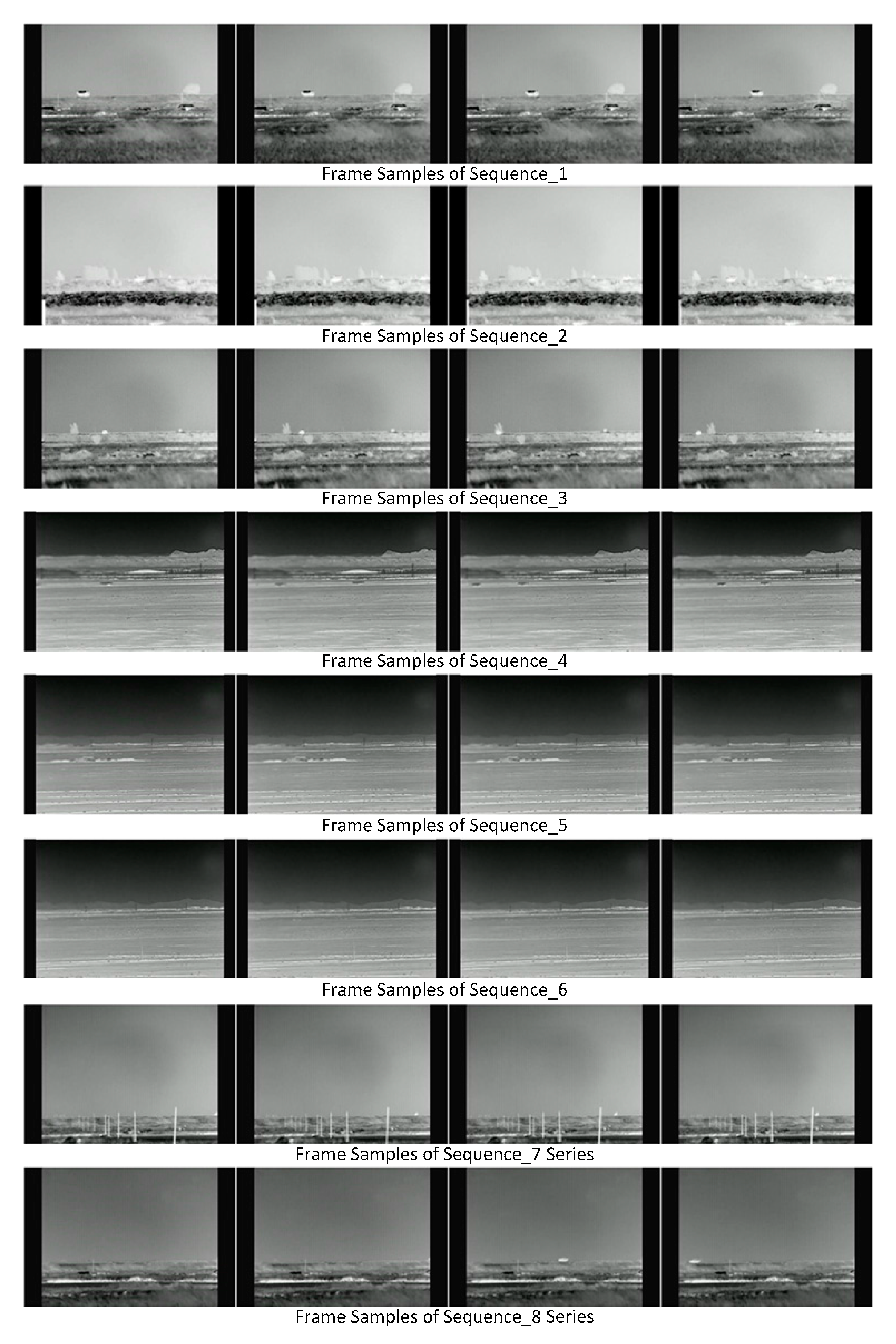
| Sequences_1 | Ghost, Dynamic Background |
| Sequences_2 | Dynamic Background, Long Time Camouflage |
| Sequences_3 | Ghost, Dynamic Background, Short Time Camouflage |
| Sequences_4 | Ghost, Device Noise, Camera Jitter |
| Sequences_5 | Small and Dim Foreground, Device Noise |
| Sequences_6 | Small and Dim Foreground, Device Noise, Camera Jitter |
| Sequence_7 series | Low Speed of Foreground Movement |
| Sequence_8 series | High Speed of Foreground Movement |
| Evaluation papers | Datasets | Evaluation Metrics |
|---|---|---|
| This Paper | Remote Scene IR Dataset | Recalld, Precisiond, F-Measured, Recalls, Precisions, F-Measures, Rankrc, Rankncr, USS, RSS, Execution Time, CPU Occupancy |
| BS | Initiation | Channels | Features | BG Model | Detection | Update |
|---|---|---|---|---|---|---|
| AdaptiveMedian | Several Frames (Detection in Initiation) | Bit-wise OR | RGB Color | Running Median | L1 Distance | Iterative |
| Bayes | One Frame | Bit-wise OR | Multi-feature Fusion (RGB Color & Color Co-occurrence) | Histogram | Probability | Hybrid (Selective & Iterative) |
| Codebook | Several Frames (No Detection in Initiation) | Bit-wise OR | YUV Color | Codeword | Minus | Selective |
| Gaussian | One Frame | Fusion | RGB Color | Statistics | L2 Distance | Iterative |
| GMG | Several Frames (No Detection in Initiation) | Fusion | RGB color | Histogram | Probability | Hybrid (Selective & Iterative) |
| GMM1 | One Frame | Fusion | RGB Color | Statistics with Weights | L2 Distance | Hybrid (Selective & Iterative) |
| GMM2 | One Frame | Fusion | RGB Color | Statistics with Weights | L2 Distance | Hybrid (Selective & Iterative) |
| GMM3 | One Frame | Fusion | RGB Color | Statistics with Weights | L2 Distance | Hybrid (Selective & Iterative) |
| KDE | Several Frames (No Detection in Initiation) | Fusion | SGR Color | Density | Probability | FIFO |
| KNN | One Frame | Fusion | RGB Color | Density | L2 Distance | Random |
| PBAS | Several Frames (Detection in Initiation) | Bit-wise OR | Multi-feature Fusion (RGB Color & Gradient) | Features Value | L1 distance | Random |
| PCAWS | One Frame | Fusion | Multi-feature Fusion (RGB Color & LBSP) | Dictionary | L1 Distance | Random |
| Sigma-Delta | One Frame | Bit-wise OR | RGB Color | Temporal Standard Deviation | L1 Distance | Iterative |
| SOBS | Several Frames (Detection in Initiation) | Fusion | HSV Color | Neuronal Map | L2 Distance | Iterative |
| Texture | One Frame | Fusion | LBP | Histograms with Weights | Histogram Intersection | Hybrid (Selective & Iterative) |
| ViBe | One Frame | Fusion | RGB Color | Features Value | L1 Distance | Random |
| BS Algorithm | Parameter Setting |
|---|---|
| AdaptiveMedian | Threshold = 20, InitialFrames = 20 |
| Bayes | Lcolor = 64, N1color = 30, N2color = 50, Lco-occurrences = 32, N1co-occurrences = 50, N2co-occurrences = 80, α1 = 0.1, α2 = 0.005 |
| Codebook | min = 3, max = 10, bound = 10, LearningFrames = 20 |
| Gaussian | InitialFrames = 20, threshold = 3.5, α = 0.001 |
| GMG | Fmax = 64, α = 0.025, q = 16, pF = 0.8, threshold = 0.8, T = 20 |
| GMM1 | Thredshold = 2.5, K = 4, T = 0.6, α = 0.002 |
| GMM2 | Thredshold = 2.5, K = 4, T = 0.6, α = 0.002 |
| GMM3 | Threshold = 3, K = 4, cf = 0.1, α = 0.001, cT = 0.01 |
| KDE | th = 10e-8, W = 100, N = 50, InitialFrames = 20 |
| KNN | T = 1000, K = 100, Cth = 20 |
| PBAS | N = 35, #min = 2, Rinc/dec = 18, Rlower = 18, Rscale = 5, Tdec = 0.05, Tlower = 2, Tupper = 200 |
| PCAWS | Rcolor = 20, Rdesc = 2, t0 = 1000, N = 50, α = 0.01, λT = 0.5, λR = 0.01 |
| Sigma-Delta | N = 4 |
| SOBS | n = 3, K = 15, ε1 = 0.1, ε2 = 0.006, c1 = 1, c2 = 0.05 |
| Texture | P = 6, R = 2, Rregion = 5, K = 3, TB = 0.8, TP = 0.65, αb = 0.01, αw = 0.01 |
| ViBe | N = 20, R = 20, #min = 2, Φ = 16 |
| BS | Prd | Red | F-md | Prs | Res | F-ms | Rankrc | Rankncr |
|---|---|---|---|---|---|---|---|---|
| AdaptiveMedian | 0.3362 | 0.2600 | 0.2933 | 0.3445 | 0.5870 | 0.3971 | 7 | 4 |
| Bayes | 0.2138 | 0.2915 | 0.2467 | 0.3527 | 0.3908 | 0.3119 | 9 | 8 |
| Codebook | 0.5759 | 0.0559 | 0.1019 | 0.5425 | 0.1038 | 0.1482 | 11 | 12 |
| Gaussian | 0.5196 | 0.1944 | 0.2829 | 0.5680 | 0.2725 | 0.3471 | 4 | 5 |
| GMG | 0.4927 | 0.0210 | 0.0402 | 0.5000 | 0.0172 | 0.0324 | 14 | 14 |
| GMM1 | 0.6838 | 0.0612 | 0.1124 | 0.7069 | 0.0720 | 0.1275 | 10 | 10 |
| GMM2 | 0.1066 | 0.5165 | 0.1767 | 0.1138 | 0.6690 | 0.1744 | 8 | 9 |
| GMM3 | 0.8121 | 0.0207 | 0.0403 | 0.8330 | 0.0181 | 0.0353 | 12 | 11 |
| KDE | 0.1976 | 0.1120 | 0.1429 | 0.1653 | 0.3086 | 0.1776 | 13 | 13 |
| KNN | 0.2408 | 0.4083 | 0.3029 | 0.3700 | 0.4690 | 0.3399 | 5 | 6 |
| PBAS | 0.6924 | 0.1279 | 0.2159 | 0.7724 | 0.1020 | 0.1716 | 6 | 7 |
| PCAWS | 0.0168 | 0.9475 | 0.0330 | 0.0058 | 0.0833 | 0.0108 | 16 | 16 |
| Sigma-delta | 0.4544 | 0.5553 | 0.4998 | 0.5200 | 0.5646 | 0.5037 | 1 | 1 |
| SOBS | 0.4548 | 0.3561 | 0.3995 | 0.4724 | 0.4673 | 0.4462 | 2 | 2 |
| Texture | 0.2431 | 0.0483 | 0.0806 | 0.3848 | 0.0584 | 0.0950 | 15 | 15 |
| ViBe | 0.3544 | 0.3526 | 0.3535 | 0.3791 | 0.63619 | 0.4318 | 3 | 3 |
| BS | Err % | SD % | D-Score 10−2 | BS | Err % | SD % | D-Score 10−2 |
|---|---|---|---|---|---|---|---|
| AdaptiveMedian | 0.244 | 0.453 | 0.177 | KDE | 0.297 | 0.382 | 0.193 |
| Bayes | 0.177 | 0.139 | 0.116 | KNN | 0.156 | 0.148 | 0.098 |
| Codebook | 1.145 | 1.030 | 0.998 | PBAS | 0.882 | 0.403 | 0.781 |
| Gaussian | 0.417 | 0.686 | 0.339 | PCAWS | 0.136 | 0.132 | 0.01 |
| GMG | 3.793 | 0.917 | 3.461 | Sigma-delta | 0.141 | 0.171 | 0.091 |
| GMM1 | 1.552 | 1.872 | 1.352 | SOBS | 0.184 | 0.196 | 0.125 |
| GMM2 | 0.136 | 0.144 | 0.05 | Texture | 0.781 | 0.422 | 0.657 |
| GMM3 | 5.487 | 2.80 | 4.892 | ViBe | 0.197 | 0.349 | 0.137 |
| Ave. F-ms | Difficulty Rank | Ave. F-ms | Difficulty Rank | ||
|---|---|---|---|---|---|
| Sequence_1 | 0.3253 | 10 | Sequence_7-1 | 0.2397 | 5 |
| Sequence_2 | 0.1025 | 3 | Sequence_7-2 | 0.2226 | 4 |
| Sequence_3 | 0.3105 | 8 | Sequence_7-3 | 0.2438 | 6 |
| Sequence_4 | 0.2630 | 7 | Sequence_8-1 | 0.3159 | 9 |
| Sequence_5 | 0.0773 | 2 | Sequence_8-2 | 0.3565 | 12 |
| Sequence_6 | 0.0297 | 1 | Sequence_8-3 | 0.3260 | 11 |
| BS + M | Prd | Red | F-md | Prs | Res | F-ms | Rankrc | Rankncr |
|---|---|---|---|---|---|---|---|---|
| AdaptiveMedian | 0.3232 | 0.3323 | 0.3277 | 0.3273 | 0.6762 | 0.3919 | 6 | 5 |
| Bayes | 0.1644 | 0.5141 | 0.2491 | 0.3008 | 0.5549 | 0.3177 | 9 | 8 |
| Codebook | 0.5735 | 0.1051 | 0.1777 | 0.5322 | 0.2380 | 0.2805 | 8 | 10 |
| Gaussian | 0.5036 | 0.2631 | 0.3456 | 0.5407 | 0.4255 | 0.4193 | 4 | 4 |
| GMG | 0.4828 | 0.0655 | 0.1154 | 0.4909 | 0.0546 | 0.0897 | 14 | 14 |
| GMM1 | 0.6826 | 0.0867 | 0.1539 | 0.6869 | 0.1496 | 0.2295 | 10 | 9 |
| GMM2 | 0.0891 | 0.5932 | 0.1549 | 0.1032 | 0.5098 | 0.1617 | 11 | 12 |
| GMM3 | 0.8344 | 0.0338 | 0.0650 | 0.8387 | 0.0336 | 0.0635 | 12 | 11 |
| KDE | 0.1847 | 0.1250 | 0.1491 | 0.1516 | 0.3866 | 0.1797 | 13 | 13 |
| KNN | 0.1871 | 0.6488 | 0.2905 | 0.3164 | 0.6249 | 0.3333 | 7 | 6 |
| PBAS | 0.6835 | 0.2117 | 0.3233 | 0.7579 | 0.1618 | 0.2500 | 5 | 7 |
| PCAWS | 0.0154 | 0.9484 | 0.0303 | 0.0053 | 0.0833 | 0.0100 | 16 | 16 |
| Sigma-delta | 0.4361 | 0.7082 | 0.5398 | 0.4918 | 0.6907 | 0.5261 | 1 | 1 |
| SOBS | 0.4441 | 0.5280 | 0.4824 | 0.4473 | 0.6169 | 0.4771 | 2 | 2 |
| Texture | 0.1493 | 0.0977 | 0.1181 | 0.3187 | 0.0956 | 0.1178 | 15 | 15 |
| ViBe | 0.3408 | 0.4553 | 0.3898 | 0.3626 | 0.6942 | 0.4294 | 3 | 3 |
| BS + MM | Prd | Red | F-md | Prs | Res | F-ms | Rankrc | Rankncr |
|---|---|---|---|---|---|---|---|---|
| AdaptiveMedian | 0.3125 | 0.4434 | 0.3666 | 0.3098 | 0.6227 | 0.3803 | 6 | 6 |
| Bayes | 0.0909 | 0.5531 | 0.1561 | 0.2193 | 0.5777 | 0.2263 | 10 | 11 |
| Codebook | 0.5521 | 0.1520 | 0.2384 | 0.5069 | 0.3992 | 0.3747 | 7 | 7 |
| Gaussian | 0.4865 | 0.3552 | 0.4106 | 0.5127 | 0.5425 | 0.4565 | 3 | 3 |
| GMG | 0.4343 | 0.1253 | 0.1945 | 0.4395 | 0.1104 | 0.1492 | 11 | 12 |
| GMM1 | 0.6559 | 0.1054 | 0.1817 | 0.6481 | 0.2251 | 0.2981 | 9 | 9 |
| GMM2 | 0.0683 | 0.6016 | 0.1227 | 0.0872 | 0.4364 | 0.1411 | 14 | 13 |
| GMM3 | 0.8260 | 0.0467 | 0.0884 | 0.8239 | 0.0608 | 0.1089 | 12 | 10 |
| KDE | 0.1675 | 0.1660 | 0.1667 | 0.1348 | 0.4266 | 0.1700 | 13 | 14 |
| KNN | 0.1130 | 0.7604 | 0.1968 | 0.2472 | 0.6180 | 0.2719 | 8 | 8 |
| PBAS | 0.6607 | 0.2952 | 0.4081 | 0.7320 | 0.2286 | 0.3310 | 5 | 5 |
| PCAWS | 0.0152 | 0.9556 | 0.0298 | 0.0052 | 0.0833 | 0.0098 | 16 | 15 |
| Sigma-delta | 0.4161 | 0.8228 | 0.5527 | 0.4674 | 0.7669 | 0.5676 | 1 | 1 |
| SOBS | 0.4245 | 0.6771 | 0.5218 | 0.4216 | 0.7371 | 0.4915 | 2 | 2 |
| Texture | 0.0896 | 0.1187 | 0.1021 | 0.2789 | 0.1114 | 0.1107 | 15 | 16 |
| ViBe | 0.3333 | 0.5788 | 0.4230 | 0.3500 | 0.6560 | 0.4298 | 4 | 4 |
| BS + M | F-md | F-mS |
|---|---|---|
| Average Improvement | 0.0369 | 0.0329 |
| Maximum Improvement | 0.1073 (PBAS) | 0.1323 (Codebook) |
| BS + MM | F-md | F-mS |
|---|---|---|
| Average Improvement | 0.0523 | 0.0479 |
| Maximum Improvement | 0.1922 (PBAS) | 0.2265 (Codebook) |
| BS | AVE. Pcj | BS | AVE. Pcj |
|---|---|---|---|
| AdaptiveMedian | −0.8732 | KDE | 0.0030 |
| Bayes | −0.4557 | KNN | 0.3918 |
| Codebook | 1.2910 | PBAS | 1.1581 |
| Gaussian | 0.9122 | PCAWS | 0.1000 |
| GMG | 0.3183 | Sigma-Delta | 0.3096 |
| GMM1 | 0.8081 | SOBS | 1.1807 |
| GMM2 | 0.2985 | Texture | 0.8852 |
| GMM3 | 0.5778 | ViBe | −0.8261 |
| Sequence_7-1 | Sequence_7-2 | Sequence_7-3 | |
|---|---|---|---|
| AdaptiveMedian | 0.3137 | 0.3157 | 0.3173 |
| Bayes | 0.3048 | 0.1358 | 0.4321 |
| Codebook | 0.6683 | 0.7034 | 0.6512 |
| Gaussian | 0.5853 | 0.5679 | 0.6069 |
| GMG | 0.6926 | 0.5737 | 0.7391 |
| GMM1 | 0.7315 | 0.7358 | 0.7389 |
| GMM2 | 0.0006 | 0.0070 | 0.0002 |
| GMM3 | 0.8646 | 0.8590 | 0.8679 |
| KDE | 0.0935 | 0.0984 | 0.0981 |
| KNN | 0.2424 | 0.1004 | 0.3442 |
| PBAS | 0.8250 | 0.8369 | 0.8331 |
| PCAWS | 0 | 0 | 0 |
| Sigma-Delta | 0.5211 | 0.4307 | 0.5720 |
| SOBS | 0.5581 | 0.5659 | 0.5542 |
| Texture | 0.2352 | 0.1576 | 0.3036 |
| ViBe | 0.3666 | 0.3617 | 0.3748 |
| Average | 0.2397 | 0.2226 | 0.2438 |
| BS | BS + M | BS + MM | |
|---|---|---|---|
| AdaptiveMedian | 0.0317 | 0.0387 | 0.0544 |
| Bayes | 0.1683 | 0.0911 | 0.0105 |
| Codebook | 0.1865 | 0.2771 | 0.3714 |
| Gaussian | 0.0964 | 0.1109 | 0.1435 |
| GMG | 0.0709 | 0.1477 | 0.1931 |
| GMM1 | 0.0572 | 0.0565 | 0.0573 |
| GMM2 | 0.0001 | 0 | 0 |
| GMM3 | 0.0421 | 0.0435 | 0.0470 |
| KDE | 0.0041 | 0.0015 | 0 |
| KNN | 0.1114 | 0.0328 | 0.0027 |
| PBAS | 0.2665 | 0.3244 | 0.3450 |
| PCAWS | 0 | 0 | 0 |
| Sigma-Delta | 0.1771 | 0.1854 | 0.1860 |
| SOBS | 0.2182 | 0.2850 | 0.3274 |
| Texture | 0.1574 | 0.1543 | 0.1008 |
| ViBe | 0.0520 | 0.0677 | 0.0899 |
| BS | BS + M | BS + MM | |
|---|---|---|---|
| Sequence_5 | 0.0773 | 0.0842 | 0.0631 |
| Sequence_6 | 0.0297 | 0.0313 | 0.0175 |
| BS | BS + M | |
|---|---|---|
| AdaptiveMedian | 0.0265 | 0.0011 |
| Bayes | 0.1036 | 0.1366 |
| Codebook | 0.0345 | 0.1412 |
| Gaussian | 0.1130 | 0.1054 |
| GMG | 0.0091 | 0.0312 |
| GMM1 | 0.0460 | 0.1108 |
| GMM2 | 0.0001 | 0 |
| GMM3 | 0.0128 | 0.0374 |
| KDE | 0.0097 | 0 |
| KNN | 0.1193 | 0.0571 |
| PBAS | 0.0708 | 0.1313 |
| PCAWS | 0 | 0 |
| Sigma-Delta | 0.1712 | 0.1086 |
| SOBS | 0.1018 | 0.0592 |
| Texture | 0.0008 | 0.0010 |
| ViBe | 0.0367 | 0.0036 |
| BS | Memory Usage | Computational Load | ||
|---|---|---|---|---|
| USS (kb) | RSS (kb) | Execution Time (ms/Frame) | CPU Occupancy 1 (%) | |
| Adaptive Median | 15,844 | 24,760 | 11.65 | 58.41 |
| GMG | 131,524 | 140,432 | 16.58 | 68.89 |
| Gaussian | 19,352 | 28,172 | 21.44 | 79.07 |
| GMM1 | 30,060 | 39,100 | 27.59 | 81.03 |
| GMM2 | 34,292 | 43,216 | 38.02 | 87.55 |
| GMM3 | 27,680 | 36,540 | 31.99 | 80.66 |
| Codebook | 102,640 | 111,328 | 6.09 | 24.18 |
| Bayes | 307,752 | 316,672 | 123.31 | 95.45 |
| KDE | 51,896 | 60,844 | 10.33 | 54.36 |
| KNN | 195,972 | 204,788 | 39.29 | 84.39 |
| PBAS | 103,336 | 112,332 | 345.73 | 97.39 |
| PCAWS | 422,696 | 431,596 | 594.84 | 98.55 |
| Sigma-Delta | 16,336 | 25,328 | 15.63 | 70.27 |
| SOBS | 74,008 | 82,824 | 223.29 | 97.13 |
| Texture | 132,192 | 14,1048 | 3157.05 | 99.64 |
| ViBe | 23,680 | 32,672 | 7.66 | 44.07 |
| BS | BS | BS + M | BS + MM | ||||||
|---|---|---|---|---|---|---|---|---|---|
| Prd | Red | F-md | Prd | Red | F-md | Prd | Red | F-md | |
| AdaptiveBGLearning | 0.556 | 0.267 | 0.361 | 0.551 | 0.378 | 0.448 | 0.535 | 0.488 | 0.511 |
| AdaptiveSelectiveBGLearning | 0.604 | 0.162 | 0.256 | 0.597 | 0.213 | 0.313 | 0.571 | 0.268 | 0.364 |
| FrameDifference | 0.213 | 0.421 | 0.283 | 0.17 | 0.601 | 0.265 | 0.11 | 0.641 | 0.188 |
| FuzzyAdaptiveSOM [64] | 0.208 | 0.323 | 0.253 | 0.202 | 0.485 | 0.285 | 0.193 | 0.649 | 0.298 |
| FuzzyChoquetIntegral [47] | 0.114 | 0.178 | 0.139 | 0.104 | 0.191 | 0.134 | 0.081 | 0.197 | 0.115 |
| FuzzyGaussian [11,73] | 0.701 | 0.05 | 0.094 | 0.704 | 0.074 | 0.135 | 0.679 | 0.092 | 0.162 |
| FuzzySugenoIntegral [74] | 0.089 | 0.226 | 0.128 | 0.081 | 0.276 | 0.125 | 0.058 | 0.306 | 0.097 |
| GMM-Laurence [40] | 0.596 | 0.163 | 0.256 | 0.589 | 0.218 | 0.318 | 0.563 | 0.277 | 0.371 |
| LOBSTER [48] | 0.206 | 0.983 | 0.34 | 0.204 | 0.985 | 0.337 | 0.202 | 0.99 | 0.335 |
| MeanBGS | 0.051 | 0.695 | 0.096 | 0.033 | 0.644 | 0.063 | 0.019 | 0.536 | 0.037 |
| MultiLayer [75] | 0.362 | 0.762 | 0.491 | 0.357 | 0.769 | 0.488 | 0.35 | 0.779 | 0.483 |
| PratiMediod [55,76] | 0.299 | 0.874 | 0.445 | 0.293 | 0.896 | 0.442 | 0.286 | 0.919 | 0.436 |
| SimpleGaussian [28] | 0.717 | 0.041 | 0.078 | 0.722 | 0.064 | 0.118 | 0.7 | 0.08 | 0.144 |
| StaticFrameDifference | 0.626 | 0.082 | 0.145 | 0.621 | 0.111 | 0.188 | 0.593 | 0.134 | 0.219 |
| SuBSENSE [68] | 0.175 | 0.989 | 0.297 | 0.174 | 0.99 | 0.295 | 0.172 | 0.991 | 0.294 |
| T2FGMM_UM [77] | 0.088 | 0.995 | 0.161 | 0.077 | 0.999 | 0.143 | 0.073 | 0.999 | 0.136 |
| T2FGMM_UV [77] | 0.605 | 0.188 | 0.286 | 0.596 | 0.32 | 0.417 | 0.566 | 0.449 | 0.501 |
| T2FMRF_UM [78] | 0.058 | 0.968 | 0.11 | 0.047 | 0.986 | 0.091 | 0.039 | 0.999 | 0.075 |
| T2FMRF_UV [78] | 0.35 | 0.534 | 0.423 | 0.343 | 0.743 | 0.469 | 0.323 | 0.855 | 0.469 |
| Texture2 [45] 2 | 0.397 | 0.344 | 0.369 | 0.39 | 0.376 | 0.383 | 0.381 | 0.406 | 0.393 |
| TextureMRF [46] | 0.356 | 0.149 | 0.21 | 0.346 | 0.167 | 0.225 | 0.335 | 0.185 | 0.238 |
| VuMeter [79] | 0.722 | 0.025 | 0.048 | 0.735 | 0.055 | 0.103 | 0.714 | 0.089 | 0.158 |
| WeightedMovingMean | 0.107 | 0.677 | 0.185 | 0.078 | 0.705 | 0.141 | 0.045 | 0.644 | 0.083 |
| WeightedMovingVariance | 0.136 | 0.624 | 0.223 | 0.109 | 0.662 | 0.188 | 0.076 | 0.63 | 0.136 |
© 2017 by the authors. Licensee MDPI, Basel, Switzerland. This article is an open access article distributed under the terms and conditions of the Creative Commons Attribution (CC BY) license (http://creativecommons.org/licenses/by/4.0/).
Share and Cite
Yao, G.; Lei, T.; Zhong, J.; Jiang, P.; Jia, W. Comparative Evaluation of Background Subtraction Algorithms in Remote Scene Videos Captured by MWIR Sensors. Sensors 2017, 17, 1945. https://doi.org/10.3390/s17091945
Yao G, Lei T, Zhong J, Jiang P, Jia W. Comparative Evaluation of Background Subtraction Algorithms in Remote Scene Videos Captured by MWIR Sensors. Sensors. 2017; 17(9):1945. https://doi.org/10.3390/s17091945
Chicago/Turabian StyleYao, Guangle, Tao Lei, Jiandan Zhong, Ping Jiang, and Wenwu Jia. 2017. "Comparative Evaluation of Background Subtraction Algorithms in Remote Scene Videos Captured by MWIR Sensors" Sensors 17, no. 9: 1945. https://doi.org/10.3390/s17091945
APA StyleYao, G., Lei, T., Zhong, J., Jiang, P., & Jia, W. (2017). Comparative Evaluation of Background Subtraction Algorithms in Remote Scene Videos Captured by MWIR Sensors. Sensors, 17(9), 1945. https://doi.org/10.3390/s17091945