Quantifying Neighborhood-Scale Spatial Variations of Ozone at Open Space and Urban Sites in Boulder, Colorado Using Low-Cost Sensor Technology

Abstract
:
1. Introduction
2. Materials and Methods
2.1. UPod Platform
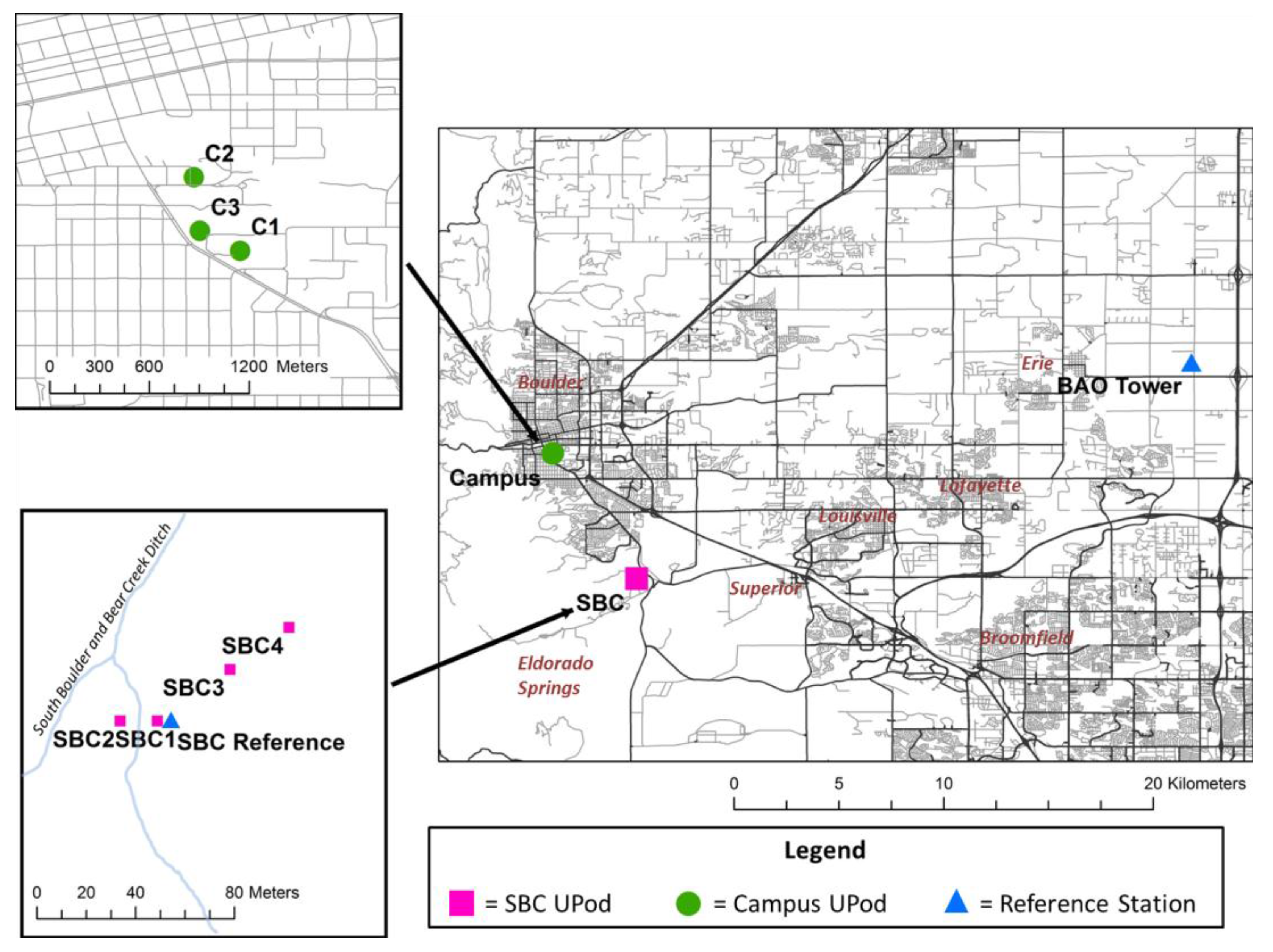
2.2. Deployments
2.3. Calibration
3. Results and Discussion
3.1. Calibration Results
3.2. Validation and Uncertainty Estimation
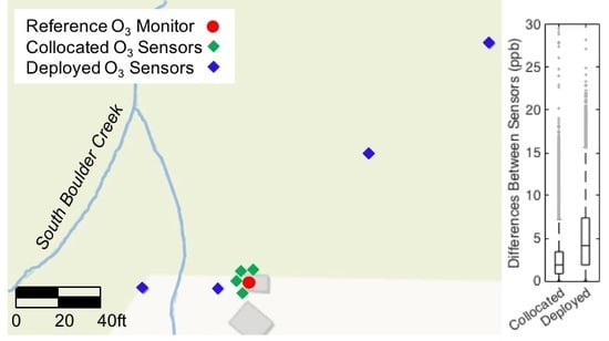
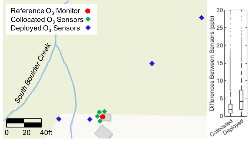
3.3. Spatiotemporal Variability
3.4. Impact of Time Averaging
4. Conclusions
Supplementary Materials
Acknowledgments
Author Contributions
Conflicts of Interest
References
- Kampa, M.; Castanas, E. Human health effects of air pollution. Environ. Pollut. 2008, 151, 362–367. [Google Scholar] [CrossRef] [PubMed]
- World Health Organization. Health Risks of Ozone from Long-Range Transboundary Air Pollution (WHO); WHO Regional Office for Europe: Copenhagen, Denmark, 2008. [Google Scholar]
- United States Environmental Protection Agency (U.S. EPA). Air Quality Criteria for Ozone and Related Photochemical Oxidants; EPA/600/R-05/004aF-cF; U.S. Environmental Protection Agency: Washington, DC, USA, 2006.
- Colorado Department of Public Health and Environment (CDPHE). Colorado Annual Monitoring Network Plan; Colorado Department of Public Health and Environment Air Pollution Control Division: Denver, CO, USA, 2015.
- Moltchanov, S.; Levy, I.; Etzion, Y.; Lerner, U.; Broday, D.M.; Fishbain, B. On the Feasibility of Measuring Urban Air Pollution by Wireless Distributed Sensor Networks. Sci. Total Environ. 2015, 502, 537–547. [Google Scholar] [CrossRef] [PubMed]
- Bart, M.; Williams, D.E.; Ainslie, B.; McKendry, I.; Salmond, J.; Grange, S.K.; Alavi-Shoshtari, M.; Steyn, D.; Henshaw, G.S. High Density Ozone Monitoring Using Gas Sensitive Semi-Conductor Sensors in the Lower Fraser Valley, British Columbia. Environ. Sci. Technol. 2014, 48, 3970–3977. [Google Scholar] [CrossRef] [PubMed]
- Jiao, W.; Hagler, G.; Williams, R.; Sharpe, R.; Brown, R.; Garver, D.; Judge, R.; Caudill, M.; Rickard, J.; Davis, M.; et al. Community Air Sensor Network (CAIRSENSE) Project: Evaluation of Low-cost Sensor Performance in a Suburban Environment in the Southeastern United States. Atmos. Meas. Tech. 2016, 9, 1–24. [Google Scholar] [CrossRef]
- Cavellin, L.D.; Weichenthal, S.; Tack, R.; Ragettli, M.S.; Smargiassi, A.; Hatzopoulou, M. Investigating the Use Of Portable Air Pollution Sensors to Capture the Spatial Variability Of Traffic-Related Air Pollution. Environ. Sci. Technol. 2016, 50, 313–320. [Google Scholar] [CrossRef] [PubMed]
- Heimann, I.; Bright, V.B.; Mcleod, M.W.; Mead, M.I.; Popoola, O.A.M.; Stewart, G.B.; Jones, R.I. Source Attribution of Air Pollution by Spatial Scale Separation Using High Spatial Density Networks of Low Cost Air Quality Sensors. Atmos. Environ. 2015, 113, 10–19. [Google Scholar] [CrossRef]
- Snyder, E.G.; Watkins, T.H.; Soloman, P.A.; Thom, E.D.; Williams, R.W.; Hagler, G.S.W.; Shelow, D.; Hindin, D.A.; Kilaru, V.J.; Preuss, P.W. The Changing Paradigm of Air Pollution Monitoring. Environ. Sci. Technol. 2013, 47, 11369–11377. [Google Scholar] [CrossRef] [PubMed]
- Williams, D.E.; Henshaw, G.S.; Bart, M.; Laing, G.; Wagner, J.; Naisbitt, S.; Salmond, J.A. Validation of Low-cost Ozone Measurement Instruments Suitable for Use in an Air-quality Monitoring Network. Meas. Sci. Technol. 2013, 24. [Google Scholar] [CrossRef]
- Kumar, P.; Morawska, L.; Martani, C.; Biskos, G.; Neophytou, M.; Sabatino, S.D.; Bell, M.; Norford, L.; Britter, R. The Rise of Low-cost Sensing for Managing Air Pollution in Cities. Environ. Int. 2015, 75, 199–205. [Google Scholar] [CrossRef] [PubMed] [Green Version]
- MacDonald, C.P.; Roberts, P.T.; McCarthy, M.C.; DeWinter, J.L.; Dye, T.S.; Vaughn, D.L.; Henshaw, G.; Nester, S.; Minor, H.A.; Rutter, A.P.; et al. Ozone Concentrations In and Around the City of Arvin, California; STI-913040-5865-FR2; Sonoma Technology: Fresno, CA, USA, 2014. [Google Scholar]
- Diem, J.E. A Critical Examination of Ozone Mapping from a Spatial-scale Perspective. Environ. Pollut. 2003, 125, 369–383. [Google Scholar] [CrossRef]
- Mobile Sensing Technology. Available online: http://mobilesensingtechnology.com/ (accessed on 1 November 2016).
- Piedrahita, R.; Xiang, Y.; Masson, N.; Ortega, J.; Collier, A.; Jiang, Y.; Li, K.; Dick, R.P.; Lv, Q.; Hannigan, M.; et al. The next Generation of Low-cost Personal Air Quality Sensors for Quantitative Exposure Monitoring. Atmos. Meas. Tech. 2014, 7, 3325–3336. [Google Scholar] [CrossRef] [Green Version]
- e2v Technologies. e2v MiCS O3 Sensor; Component Distributors, Inc.: Denver, CO, USA, 2008; Available online: https://www.cdiweb.com/datasheets/e2v/mics-2610.pdf (accessed on 10 September 2016).
- Williams, D.E.; Henshaw, G.; Wells, D.B.; Ding, G.; Wagner, J.; Wright, B.; Yung, Y.F.; Akagi, J.; Salmond, J. Development of Low-Cost Ozone and Nitrogen Dioxide Measurement Instruments Suitable for Use in An Air Quality Monitoring Network. ECS Trans. 2009, 19, 251–254. [Google Scholar]
- Masson, N.; Piedrahita, R.; Hannigan, M. Approach for Quantification of Metal Oxide Type Semiconductor Gas Sensors Used for Ambient Air Quality Monitoring. Sens. Actuators B Chem. 2015, 208, 339–345. [Google Scholar] [CrossRef]
- MaxDetect Technology Co., Ltd. Digital Relative Humidity & Temperature Sensor RHT03. Available online: http://cdn.sparkfun.com/datasheets/Sensors/Weather/RHT03.pdf (accessed on 17 February 2017).
- Colorado Department of Transportation (CDOT). Traffic Data Explorer. Online Transportation Information System 2017. Available online: http://dtdapps.coloradodot.info/otis/TrafficData (accessed on 15 May 2017).
- McClure-Begley, A.; Petropavlovskikh, I.; Oltmans, S. NOAA Global Monitoring Surface Ozone Network, June-July 2015, BAO Tower; National Oceanic and Atmospheric Administration, Earth Systems Research Laboratory Global Monitoring Division: Boulder, CO, USA, 2015. [CrossRef]
- Galbally, I.E.; Schultz, M.G.; Buchmann, B.; Gilge, S.; Guenther, F.; Koide, H.; Oltmans, S.; Patrick, L.; Scheel, H.-E.; Smit, H.; et al. Guidelines for Continuous Measurements of Ozone in the Troposphere; WMO-No. 1110; World Meteorological Organization: Geneva, Switzerland, 2013. [Google Scholar]
- United States Environmental Protection Agency (U.S. EPA). Transfer Standards for Calibration of Air Monitoring Analyzers for Ozone; EPA-454/B-13-004; U.S. Environmental Protection Agency: Research Triangle Park, NC, USA, 2013.
- Murphy, D.M.; Koop, T. Review of the vapour pressures of supercooled water for atmospheric applications. Q. J. R. Meteorol. Soc. 2005, 131, 1539–1565. [Google Scholar] [CrossRef]
- Brodin, M.; Helmig, D.; Oltmans, S. Seasonal ozone behavior along an elevation gradient in the Colorado Front Range Mountains. Atmos. Environ. 2010, 44, 5305–5315. [Google Scholar] [CrossRef]
- Lippmann, M. Health Effects of Ozone A Critical Review. J. Air Waste Manag. Assoc. 1989, 39, 672–695. [Google Scholar] [CrossRef]
- United States Environmental Protection Agency (U.S. EPA). Final Report: Integrated Science Assessment of Ozone and Related Photochemical Oxidants; EPA/600/R-10/076F; U.S. Environmental Protection Agency: Washington, DC, USA, 2013.


| Ozone Instrument Name | Instrument Type | Latitude | Longitude | Location Altitude (m above sea level) | Location Description | Inlet Height (m above ground) | Collocation/Deployment |
|---|---|---|---|---|---|---|---|
| Boulder Atmospheric Observatory (BAO) Tower | UV Absorption Analyzer | 40.0500 | −105.0004 | 1584 | Tall tower operated by the National Oceanic and Atmopsheric Administration (NOAA) | 6 | Collocation |
| SBC-Ref | Photometric Ozone Analyzer | 39.9572 | −105.2385 | 1671 | Colorado Department of Public Health and Environment (CDPHE) monitoring site | 4.3 | Collocation |
| C1 | Metal Oxide Sensor | 40.0069 | −105.2720 | 1667 (including 15 m from ground to rooftop) | University Memorial Center building—rooftop | 1.5 | Collocation (at BAO) and Deployment |
| C2 | Metal Oxide Sensor | 40.0109 | −105.2745 | 1655 (including 10 m from ground to rooftop) | Continuing Education building—western rooftop | 1.5 | Collocation (at BAO) and Deployment |
| C3 | Metal Oxide Sensor | 40.0080 | −105.2742 | 1666 (including 9 m from ground to balcony | Geography building—south balcony | 1.5 | Collocation (at BAO) and Deployment |
| SBC1 | Metal Oxide Sensor | 39.9572 | −105.2386 | 1671 | SBC—nearest to reference monitor | 1.5 | Collocation (at SBC) and Deployment |
| SBC2 | Metal Oxide Sensor | 39.9572 | −105.2387 | 1671 | SBC – nearest to trees and more dense foliage | 1.5 | Collocation (at SBC) and Deployment |
| SBC3 | Metal Oxide Sensor | 39.9575 | −105.2381 | 1671 | SBC—nearest to road | 1.5 | Collocation (at SBC) and Deployment |
| SBC4 | Metal Oxide Sensor | 39.9574 | −105.2383 | 1671 | SBC | 1.5 | Collocation (at SBC) and Deployment |
| Segment of Collocation | Pod ID | R2 with Reference Instrument | RMSE with Reference Instrument (ppb) |
|---|---|---|---|
| Calibration Generation Period | SBC1 | 0.95 | 3.2 |
| SBC2 | 0.95 | 3.2 | |
| SBC3 | 0.97 | 3.0 | |
| SBC4 | 0.93 | 5.0 | |
| C1 | 0.91 | 2.9 | |
| C2 | 0.91 | 2.4 | |
| C3 | 0.92 | 2.5 | |
| Validation Data Period | SBC1 | 0.90 | 5.9 |
| SBC2 | 0.95 | 4.3 | |
| SBC3 | 0.92 | 5.3 | |
| SBC4 | 0.73 | 12.3 |
| Pod ID | Median Ozone (ppb) | 95th Percentile Ozone (ppb) | ||||
|---|---|---|---|---|---|---|
| Minute | Hour | 8-h | Minute | Hour | 8-h | |
| SBC1 | 35 | 36 | 35 | 65 | 65 | 58 |
| SBC2 | 40 | 39 | 39 | 66 | 66 | 59 |
| SBC3 | 33 | 33 | 32 | 58 | 57 | 53 |
| C1 | 51 | 51 | 50 | 93 | 93 | 83 |
| C2 | 39 | 39 | 40 | 83 | 83 | 75 |
| C3 | 39 | 39 | 39 | 87 | 87 | 76 |
© 2017 by the authors. Licensee MDPI, Basel, Switzerland. This article is an open access article distributed under the terms and conditions of the Creative Commons Attribution (CC BY) license (http://creativecommons.org/licenses/by/4.0/).
Share and Cite
Cheadle, L.; Deanes, L.; Sadighi, K.; Gordon Casey, J.; Collier-Oxandale, A.; Hannigan, M. Quantifying Neighborhood-Scale Spatial Variations of Ozone at Open Space and Urban Sites in Boulder, Colorado Using Low-Cost Sensor Technology. Sensors 2017, 17, 2072. https://doi.org/10.3390/s17092072
Cheadle L, Deanes L, Sadighi K, Gordon Casey J, Collier-Oxandale A, Hannigan M. Quantifying Neighborhood-Scale Spatial Variations of Ozone at Open Space and Urban Sites in Boulder, Colorado Using Low-Cost Sensor Technology. Sensors. 2017; 17(9):2072. https://doi.org/10.3390/s17092072
Chicago/Turabian StyleCheadle, Lucy, Lauren Deanes, Kira Sadighi, Joanna Gordon Casey, Ashley Collier-Oxandale, and Michael Hannigan. 2017. "Quantifying Neighborhood-Scale Spatial Variations of Ozone at Open Space and Urban Sites in Boulder, Colorado Using Low-Cost Sensor Technology" Sensors 17, no. 9: 2072. https://doi.org/10.3390/s17092072