Dual Channel S-Band Frequency Modulated Continuous Wave Through-Wall Radar Imaging


1
Department of Electronic Engineering, Hanyang University, Seoul 04763, Korea
2
Collaborative Robots Research Center, Daegu Gyeongbuk Institute of Science and Technology, Daegu 42988, Korea
*
Author to whom correspondence should be addressed.
Sensors 2018, 18(1), 311; https://doi.org/10.3390/s18010311
Submission received: 6 December 2017
/
Revised: 12 January 2018
/
Accepted: 16 January 2018
/
Published: 22 January 2018
(This article belongs to the Section Remote Sensors)
Abstract
:This article deals with the development of a dual channel S-Band frequency-modulated continuous wave (FMCW) system for a through-the-wall imaging (TWRI) system. Most existing TWRI systems using FMCW were developed for synthetic aperture radar (SAR) which has many drawbacks such as the need for several antenna elements and movement of the system. Our implemented TWRI system comprises a transmitting antenna and two receiving antennas, resulting in a significant reduction of the number of antenna elements. Moreover, a proposed algorithm for range-angle-Doppler 3D estimation based on a 3D shift invariant structure is utilized in our implemented dual channel S-band FMCW TWRI system. Indoor and outdoor experiments were conducted to image the scene beyond a wall for water targets and person targets, respectively. The experimental results demonstrate that high-quality imaging can be achieved under both experimental scenarios.
1. Introduction
Through-the-wall radar (TWR) techniques have been investigated in the past few years as a way to support police and soldiers operating in urban areas (e.g., when breaking into a room occupied by hostile agents) and to help first responders in search and rescue operations (e.g., when looking for people trapped inside buildings on fire or buried under rubble).
When the transmitted TWR signal encounters a wall, most of the transmitted signals are reflected due to the short wavelength of the transmitted signal in comparison with the dimensions of the wall. In TWR systems, the reflected signals from the wall are much stronger than those from the targets behind the wall. The presence of strong undesired signals limits the dynamic range of TWR systems and increases the possibility of saturation and blocking of the receiver [1]. Furthermore, it has been observed that this prevents the application of compressive sensing techniques, which aim at producing radar images of the same quality and resolution using far fewer data, thus allowing faster measurements [2].
In recent decades, TWR systems have been used to detect and track targets behind walls by estimating the distance and velocity of targets [3,4]. However, especially in rescue missions, surveillance, and reconnaissance, the exact locations of targets are urgently needed. Thus, through-the-wall radar imaging (TWRI) has been recently sought out to image the relative position, illustrated by down-range and cross-range, in a certain coordinate system [5,6,7].
There are several waveforms utilized in TWRI systems, including pseudo-noise waveforms based on M-sequences [8], stepped-frequency continuous wave (SFCW) signals [9,10,11], and frequency-modulated continuous wave (FMCW) signals [12,13,14,15,16].
Several prototypes of TWRI systems using UWB impulses have been developed [17,18,19] due to their high resolution in time delay estimation. However, UWB impulse radar is very complex, especially in the design of signal processing platforms, due to the high sampling rate of ADC which is proportional to signal bandwidth. In contrast, even if the bandwidth of FMCW radar is the same as that of UWB pulse radar, FMCW radar can be implemented at low cost due to its low sampling rate as compared with that of UWB pulse radar.
The FMCW radar is a cost effective alternative to high resolution radar. Because of their low complexity and low sampling rates, FMCW radars are inexpensive and easy to manufacture, relatively free from failure, and cheap to maintain. Thus, the FMCW technique was adopted in this article.
Among the many interesting aspects of TWRI, such as wall parameter estimation [20], wall clutter mitigation [5] and compensation of the angle estimations due to the wall [6], our research interest is only focused on target imaging behind walls.
Most of the TWRI systems [1,21,22] using FMCW signals adopt synthetic aperture radar (SAR) signal processing, which requires a movement of the radar and a huge amount of data processing. Thus, even though SAR yields a high quality TWRI, SAR-based TWRI systems may not be suitable in situations in which information regarding what is behind walls must be obtained rapidly, i.e., terror attacks, military purposes, rescue situations, etc.
A low complexity TWRI system using FMCW signals is presented in this article. Our developed TWRI system is equipped with one transmitting antenna, Tx, and two receiving antennas, Rx. Based on this two-receiving-antenna structure, we proposed an optimized dual channel TWRI algorithm, which exploits a 3D shift-invariant structure in 3D range-angle-Doppler subspace, resulting in high resolution images of targets. Compared with previously developed TWRI systems, our TWRI system is realized with low complexity, using only two channels. Finally, experimental trials were conducted, and the results demonstrated the high performance of our developed low complexity TWRI system and the proposed high resolution subspace algorithm.
2. System Model
Prior to introducing the proposed algorithm for low complexity TWRI, the fundamentals of the system model for TWRI and the simplified signal model for the algorithm are presented, respectively, in this section.
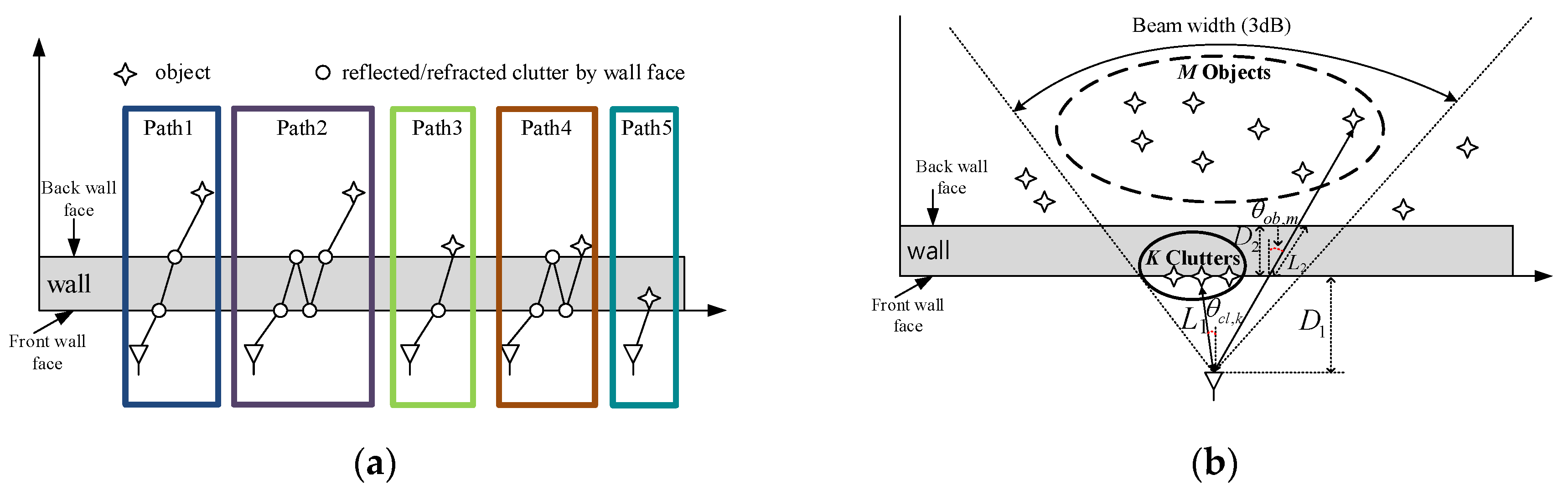
In the TWRI system literature [6,23,24,25,26], a variety of wave propagation models have been studied. Summarizing the suggested models in previous articles, five propagation models are described in Figure 1a, including reflection, refraction and wall ringing within a wall. Path 1 and path 2 show that a wave penetrates the wall and is reflected by an object behind wall, accompanied by refraction in path 1 and wall ringing within the wall in path 2. In contrast, paths 3 to 5 are caused by clutters on front/back face of the wall. As a simplification of practical signal model for TWRI systems introduced in [26], we adopt a simplified signal model including paths 1 and 5 in this paper as shown in Figure 1b. The transmitted signal is propagated along the direct path between an antenna and an object, without consideration of the refraction on the interface between the wall and air. Meanwhile, for the undesired clutter signal we only focus on that reflected by the front face of the wall.
Related to TWRI, a lot of research areas have been explored in previous works, including wall parameter estimation [20], compensation for refraction due to the wall [6], SAR for high resolution [22], and so far. Since we focused on presenting a low complexity TWRI algorithm, the other research topics related to TWRI are not addressed in this paper.
Let us denote the number of wall clutters and the number of the objects behind walls in the field of view, K and M, respectively, as shown in Figure 1b.
The round-trip delay (RTD) of the k-th clutters τcl,k can be obtained by:
where L1 is the standoff distance between the antenna and clutters at the front face of the wall, c is the speed of light in free space, and θcl,k is the direction of arrival (DOA) of received signal from k-th clutter.
Assuming that the m-th object at the direct path distance Rm away from the antenna is moving with a constant radial velocity vm over P pulses, the direct path distance between the antenna and the m-th object for the p-th pulse is changed to:
where TPRI is the pulse repetition interval (PRI). Thus, the RTD of the m-th object for the p-th pulse can be obtained as in [26] such that:
where D is the thickness of the wall, and ε is the dielectric constant of the wall. It can be easily derived that τob,p,m τcl,k in proportional to D and ε by comparing τob,p,m of Equation (3) with τcl,k of Equation (1).
Rp,m = Rm + vm × pTPRI
The transmitted P FMCW chirp pulses can be modeled by:
fc denotes the carrier frequency, μ is the rate of change of the instantaneous frequency of a chirp signal, and Tsym is the duration of the FMCW chirp pulse. The bandwidth of the FMCW chirp signal is defined by fBW = μTsym/2π.
Considering two receiving antennas, separated by a distance d, the received p-th pulse at the l-th antenna can be represented from the TWRI simplification of [26] by:
where acl,k and aob,m denote the complex amplitude for the k-th clutter and the m-th object, respectively, and λs denotes the wavelength of the carrier signal, for l = 0 and 1.
In an FMCW radar, received chirp signals can be easily transformed into a sinusoidal waveform by de-chirping, which involves multiplying the received signal by the transmitted chirp replica, followed by low-pass filtering [16], as shown in Figure 2b. We call these sinusoids beat signals. The p-th beat signal at the l-th antenna can be represented as in [16] by:
where fcl,k and fob,p,m are the frequencies of the transformed beat signals from the wall clutter and object, respectively, by:
In a through-wall radar imaging scenario, the speed of the objects v is assumed to be much smaller than that of vehicles. Thus, the effects of the movement over P pulses on the complex amplitude and DOA can be ignored as in Equation (3), Equation (5), and Equation (8). We only considered it in RTD as in Equation (8).
Substituting τob,p,m with Rp,m of Equation (2) in Equation (8), the beat signals from an object behinds wall can be modeled with some approximation of [27], by
where ηm denotes the fixed phase term for the m-th object, induced in the process of approximation.
Generally, the two-way loss due to a wall can be represented by
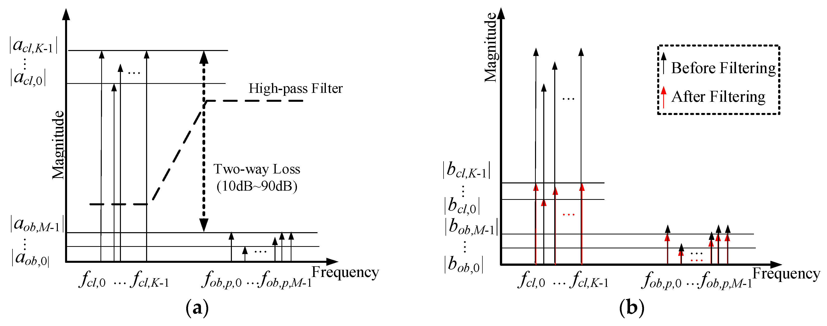
and the loss is determined by the material and thickness of the wall. In the case of a reinforced concrete wall, a 20 cm thickness yields 90 dB two way loss as in [16]. From the relationship of τob,p,m τcl,k, the frequency of the transformed beat signals also can be related to each other, such that, fob,p,m fcl,k. If the frequencies for clutters and objects can be grouped separately from each other because of the wall, as shown in Figure 2a, a low pass filter can be applied with the beat signals to reduce the gap between |acl,k| and |aob,m|, as illustrated in Figure 2. If the gap is not reduced in the specific case of reinforced concrete wall of 20 cm, most of the dynamic range of ADC is fit to the magnitude level of wall clutter, |acl,k|. This causes the SNR for the digitized samples for the beat signals from the M objects to be very poor due to two-way loss, leading to missed detection. Thus, most conventional FMCW through wall radar systems make use of a high-pass filter to reject the wall-induced components.
The magnitudes |acl,k| and |aob,m| in Figure 2a are replaced with |bcl,k| and |bob,m| in Figure 2b to describe the filtered beat signals. Since a high-pass filter is used for wall clutter rejection, |acl,k| |bcl,k| and |aob,m||bob,m|.
After analog-to-digital conversion, the discrete time model for rp,l(t) of Equation (5) with the sampling frequency fs = 1/Ts satisfying the Nyquist criterion can be derived by yp,l [n] = yl (nTs) for p = 0,…, P − 1, l = 0 and 1, and n = 0,..., N − 1, where N = Tsym/Ts.
3. Conventional FMCW TWRI Systems
In previous works [28,29,30,31,32,33], many methods and architectures have been proposed for TWRI systems based on SFCW or FMCW signals, as well as synthetic aperture radar (SAR) principles. These conventional works on TWRI systems are briefly summarized in this section.
3.1. Subspace Projection Approach
The eigenstructure of the imaged scene is obtained by performing the SVD of Z:
where H denotes the Hermitian transpose, U and V are unitary matrices containing the left and right singular vectors, respectively, is a diagonal matrix:
and are the singular values. The subspace projection method assumes that the wall returns and the target reflections lie in different subspaces. Since the wall reflections are stronger than the target returns, the first J dominant singular vectors of the Z matrix are used to construct the wall subspace [29].
3.2. SAR-Based Approach
In [30,31,32,33], the SAR principle is used to extend standard radar imaging to account for the presence of the wall in the TWRI system. The novel combination of FMCW technology and SAR techniques leads to the development of a small, lightweight, and cost-effective high resolution imaging sensor. In [30], an algorithm for processing FMCW SAR signals is presented; however, it requires the complete bandwidth of the transmitted signal to be sampled and a single long FFT to be performed over all of the collected data for the processing. FMCW radar technology is of interest for both civil and military airborne Earth observation applications, especially in combination with high resolution SAR techniques.
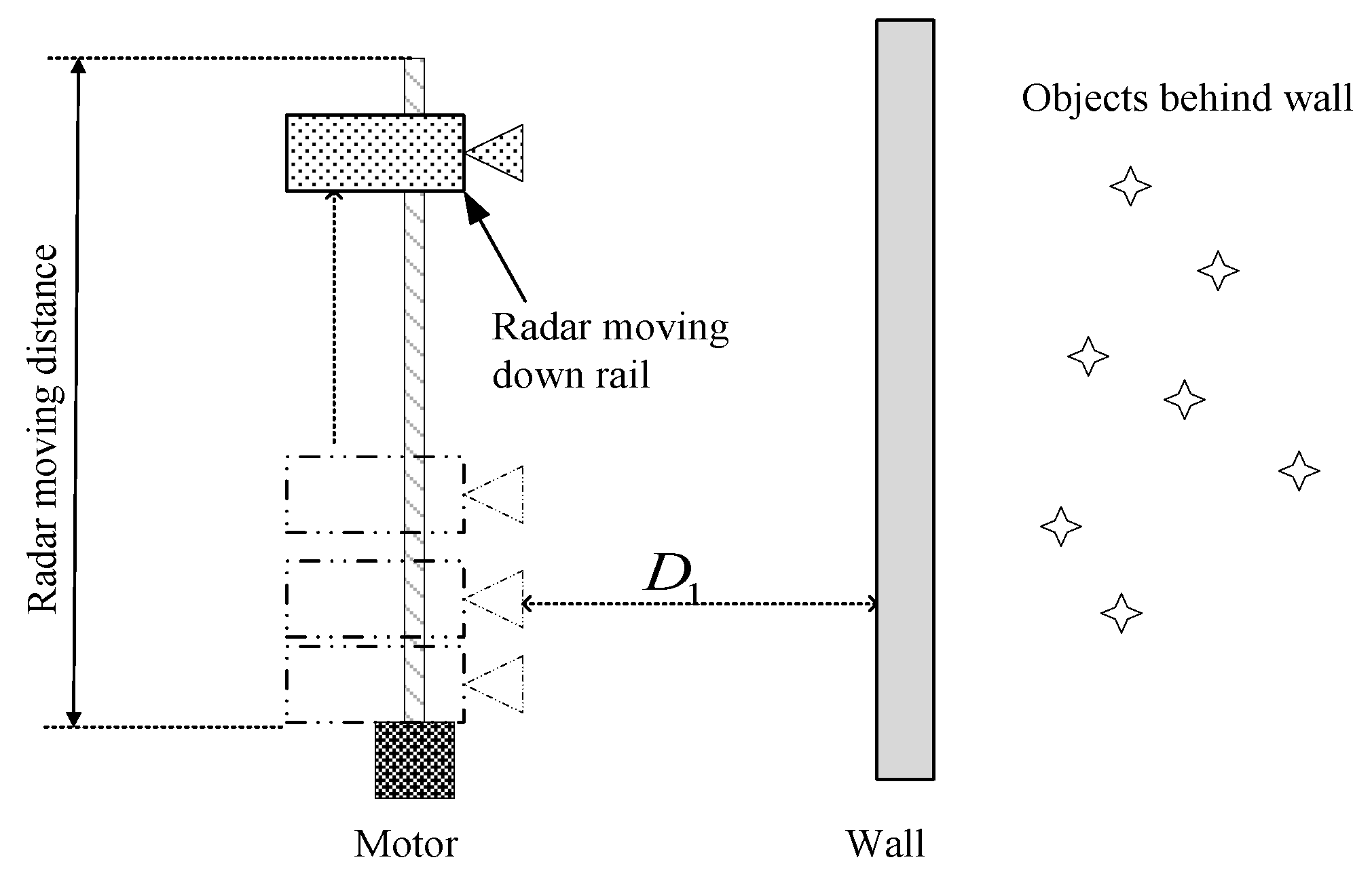
In Figure 3, a typical SAR-based TWRI geometry, in which FMCW radar is mounted on a moving platform equipped with a motor, is presented from [31].
This kind of SAR-based TWRI system is not suitable in emergency situations such as terror attacks and rescue missions because the entire SAR system cannot be conveniently transported. Moreover, conventional SAR-based TWRI systems [31,32,33] are developed with many antennas for the realization of high quality imaging.
Unlike the conventional SAR-based FMCW systems with several antennas for high quality imaging, in this paper, a dual channel S-band FMCW TWRI system is proposed for low complexity realization and high mobility.
4. 3D Subspace-Based TWRI Algorithm
For high resolution TWRI with two receiving antennas without movement for the SAR approach, the 3D subspace-based algorithm is presented with the beat samples, yp,l[n] = yp,l(nTs) for p = 0,…, P − 1, l = 0 and 1, and n = 0,..., N − 1. The main principle of the propose method is related to the 3D shift invariant structure of the matrix of Equation (18), stacked in column direction.
4.1. Phase Shift Characteristics
Before describing the principle of the proposed method, we present the phase relationships of the beat samples yp,l [n] between the adjacent samples, the adjacent pulses, and the adjacent antennas, in association with range, Doppler and angle, respectively. For the convenience of describing the phase shifts without loss of generality, we assume a single object environment, i.e., K = 0 and M = 1 in Equation (6). In this condition where no wall clutter is assumed, yp,l[n] = bob(nTs) from Equations (6)–(8). Then, three kinds of the phase shifts, κm, ξm and ρm can be defined from the approximated model for bob(nTs) in Equation (10) as follows:
- Range-induced phase shift κm:
- DOA-induced phase shift ξm:
- Doppler-induced phase shift ρm:
4.2. 3D Smoothed Hankel Matrix
Since the goal of the proposed method is to estimate range, angle and Doppler jointly, the 3D shift invariant matrix is employed for 3D subspace-based processing.
By stacking the Hankel matrices in a specific way, the 3D shift invariant structure is satisfied for the sample, pulse, and antenna domain, respectively.
Prior to introducing the 3D shift invariant structure, a 1D shift invariant structure realized by a 1D smoothed Hankel matrix is demonstrated as follows.
For yp,l[n], n = 0,…, N − 1, l = 0, 1, the single smoothed Hankel matrix Yp,l can be made as:
where denotes the complex matrix space of a by b, and Lr and Lc = N − Lr + 1 are the selection parameters, referred to as pencil parameter in [34], which satisfy the conditions Lr ≥ M and Lc ≥ M. Shifting the Hankel matrix in Equation (18) up (dropping the first row) or down (dropping the last row) results in a matrix with a row space that lies within the row space of the original matrix, which indicates that the row space of the matrix in Equation (18) is a shift-invariant subspace.
A 2D smoothed matrix Yl is obtained by stacking single smoothed Hankel matrices Yp,l:
Shifting the matrix in Equation (19) up (dropping the first matrix Y0,l) or down (dropping the last matrix YP−1,l) results in a matrix with a row space that lies within the row space of the original matrix in Equation (19), which indicates that the row space of the matrix in Equation (19) is also a shift-invariant subspace.
Obviously, matrices Yl share one identical row space. Namely, for the matrix formed by stacking Yl column, when l = 0, 1,.., L − 1, dropping the first segment Y0 or dropping the last matrix YL−1 results in a matrix with a row space that lies within the row space of the original matrix. In our proposed FMCW TWRI system, the number of receive antennas is two, which makes for a special 3D smoothed matrix case with only two segments:
Conventional subspace-based algorithms such as Matrix Pencil [34] make use of a 1D Shift Structure to obtain the frequency estimation. Like conventional algorithms, three frequency parameters κm, ξm and ρm need to be estimated in our proposed FMCW TWRI system; a 3D Shift Invariant Structure is proposed, which is formed by organizing a 3D smoothed Hankel matrix, as shown in Figure 4.
4.3. Subspace Separation with SVD
The matrix Y in Equation (20) is factored by singular value decomposition (SVD) such that:
In Equation (21), the submatrices Us, Σs, and Vs are associated with the signal subspace, and the submatrices Us, Σs, and Vs are associated with the noise subspace. The signal subspace and noise subspace are defined by:
After SVD on Y, the matrices U, Σ, and V are given as a pair. However, the separation of Equation (22) is not automatically supported by SVD; the derived singular values must be used in a specific manner. The criterion of the minimum description length (MDL) [35] is adopted in this paper for classification of the signal and noise subspaces shown in Equation (22).
Assuming noiseless data for convenience, we have:
For smoothed Hankel matrix Yp,l a steering matrix A1D with Vandermonde structure is defined in terms of the components of the M sinusoids of yp,l(t) by:
Assuming a noiseless matrix Yp,l for convenience, a basis for the column space for Yp,l of rank M can be defined as the set of columns in A since the phase shift κm corresponds to the phase shift of yp,l(t). Thus, there exists a transformation matrix F of M by Lr satisfying Yp,l = A1DF as in [36]. Similarly, for 2D stacked matrix Yl we have Yl = A2D,lF, and A2D,l is defined as:
where:
and diag[·] denotes the diagonal matrix.
Finally, the 3D stacked matrix Y is represented as:
where
Assuming that the estimated signal subspace Us is correctly separated from the noise subspace, there can be the following relationship between A3D of Equation (26) and Us, such that:
where T is an M by M non-singular transformation matrix, as in [36]. Since M objects are assumed in Equation (5), Us, the spanning signal subspace, also has M basis vectors. Thus, the steering matrix A3D, which is composed of M column vectors as in Equation (26), is related to Us by Equation (27).
4.4. 3D Pseudo-Spectrum for TWRI
Since the signal subspace and noise subspace are orthogonal, we propose a 3D pseudo-spectrum estimation for three kinds of phase shifts, κm, ξm and ρm.
Assuming three pseudo-spectrum steering vectors are defined such that:
for q = 0,…, Q − 1, w = 0,…, W − 1, and g = 0,…, G − 1, respectively.
The 3D pseudo-spectrum can be obtained through the vector s (q, w, g) and the signal subspace spanning matrix Us in Equation (23), such as:
where s(q,w,g) = sqswsg, and denotes the Kronecker product.
By the peak detection method, the M peaks can be detected for each 1D pseudo-spectrum searching, and the estimated three indexes at which the M peaks are found, such that:
where maxm[•] denotes the m-th biggest value. Since the three indexes of 3D pseudo-spectrum are estimated, estimations for the ranges, DOAs and velocities of M objects behind the wall, can be organized by the relationship in κm, ξm and ρm in Equations (15)–(17), for m = 0,…, M − 1, respectively:
5. Experiments
A concise and precise description of the experimental results will be presented. This section is divided into two subsections.
5.1. Experiment Setup
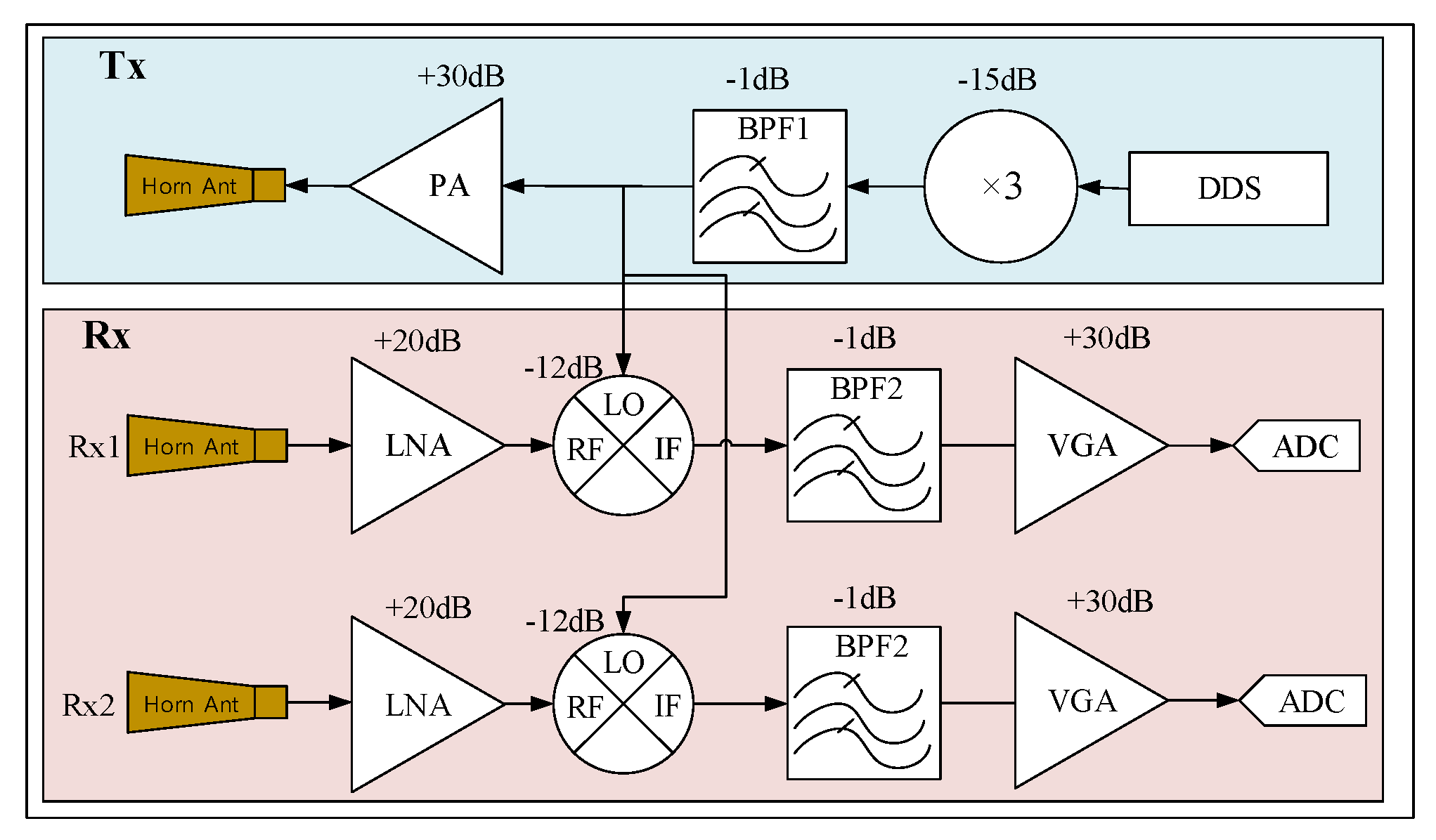
We implemented the proposed S-band FMCW TWRI radar system at 2.9 GHz, which has two receiving antennas and 2 ADC channels. As illustrated in Figure 5, the beat signals from the two ADC channels, which are connected to the two receiving antennas, respectively, were used with the proposed method and the conventional algorithms for imaging.
The transmitter constitutes of an AD9914 Direct Digital Synthesizer (DDS) from Analog Devices (Norwood, MA, USA), a Band Pass Filter (BPF), a frequency multiplier with a multiplication factor of 3, and a Power Amplifier (PA). The AD9914 generates the FMCW source, sweeping over the range from 867 MHz to 1067 MHz, that is, a 200 MHz bandwidth. Through the frequency tripler, the transmitted signal of 2.6 GHz to 3.2 GHz with bandwidth B = 600 MHz is obtained. Following the frequency tripler, BPF1, with a frequency range 2.6 GHz to 3.2 GHz is employed to optimize the generated Tx signal. In our TWRI system, the other parameters are set as follows: TPRI = 200 μs, fc = 2.9 GHz, fs = 12.5 MHz, N = 2048, P = 10, Lc = 1000, and Lr = 1049.
The receiver comprises two LNAs, two mixers, two BPFs, two VGAs and two 12-bit ADCs. For each Rx channel, one of LNAs will amplify the RF signal with a gain of 20 dB. The amplified RF signal is downconverted to an IF signal (beat signal) by the mixer with a gain of −12 dB. Due to the frequency components induced by the wall, BPF2 is utilized to inject those frequency components, as stated in Section 2. The measured 3 dB cutoff frequency of the BPFs is about 40 KHz. In the implemented system, we sampled the received signal at 13.3 MHz. The gain of single modules are shown in Figure 5.
The very significant application in our TWRI system is the implementation of a high-pass filter. In our implemented system, we use one bandpass filter with a 132 KHz to 2640 KHz BP, as shown in Figure 6a, instead of the conceptual high-pass filter shown in Figure 2. Due to the response of the band-pass filter shown in Figure 6b, this filter can filter the frequency component mainly induced by the concrete wall. As mentioned previously, we concentrate on the imaging of a target behind a wall. Although this BP filter is sufficient for frequency component rejection due to the wall clutter, we applied one subspace projection approach in [29] to our real experiments to mitigate the remaining and dominant frequency components due to wall clutter.
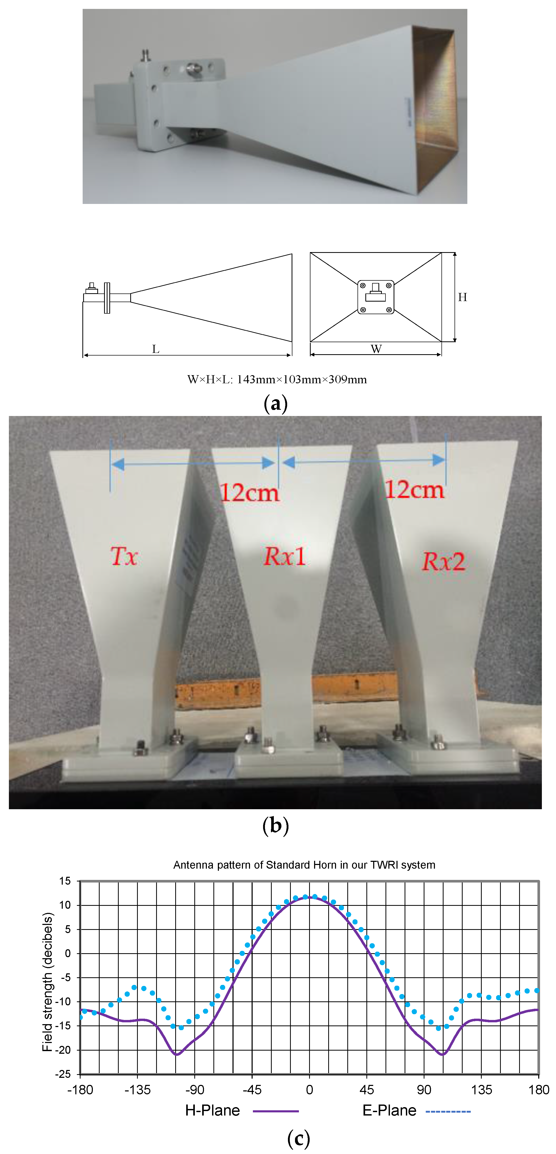
Three identical standard horn antennas with 10 dB gain were employed in our implemented system, one for Tx (Back-end) and the others for Rx1 and Rx2 (Front-end), respectively. The outline and beam patterns of the standard horn antennas are illustrated in Figure 7a. The three centers of the antennas are assigned with equivalent distances of 12 cm, as show in Figure 7b.
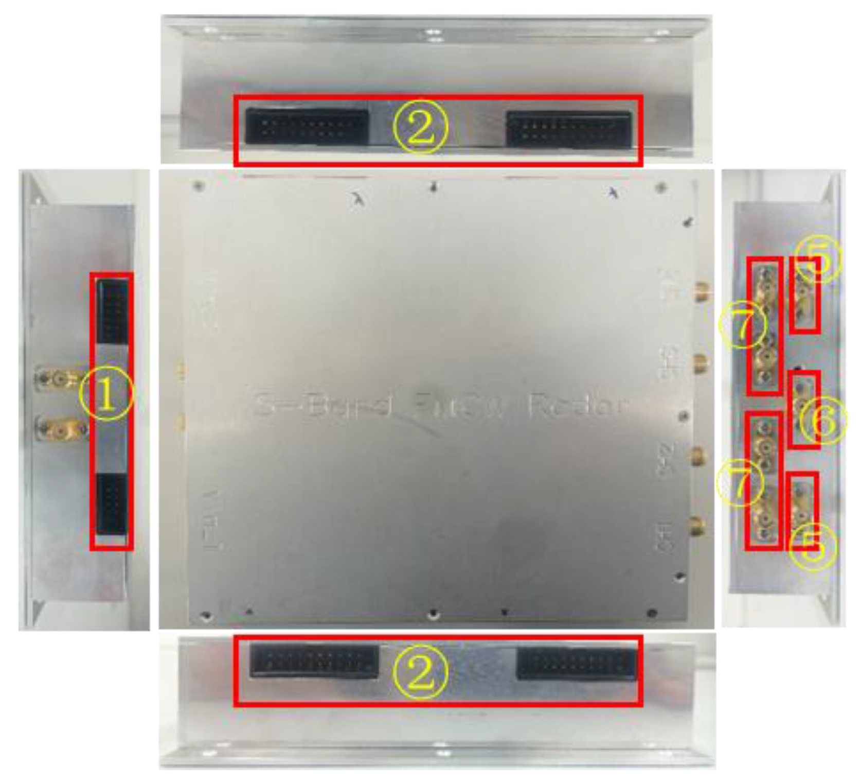
The distance between two Rx antennas approximately equaled to λ, resulting in a beamwidth covering the range from −30° to 30°, which matches the E-plane pattern (51.32°) of standard horn antenna shown in Figure 7c. Figure 7c shows the measured radiation pattern on the E plane at 24 GHz of the transmitting antenna and a receiving antenna in the anechoic chamber. The radiation pattern of the used standard horn antenna is shown in Figure 7c, having HPBW of 92° between 42.6° and 330° and an antenna gain of 11.6 dBi. The implementation of our S-Band FMCW TWRI radar system is shown in Figure 8 and Figure 9 based on the block diagram of Figure 5.
The received beat signal was sampled through an FPGA and a DSP board (see Figure 10). The ADC in the implemented radar system has a 12-bit output, and a 12.5 MHz sampling rate. Given that the rule of thumb is that every bit of an ADC represents 6 dB of a dynamic range, the 12-bit ADC provides a 72-dB dynamic range.
After taking system/subsystem issues into account, the specifications of our implemented system are summarized in Table 1.
5.2. Experiment Results
Experiments were conducted to test the developed TWRI system. Our FPGA-DSP board is configured to have a 2048-points sample number and a sampling rate of 12.5 MHz. The results were produced by the MATLAB implementation for a particular test data set sampled by the FPGA and DSP board.
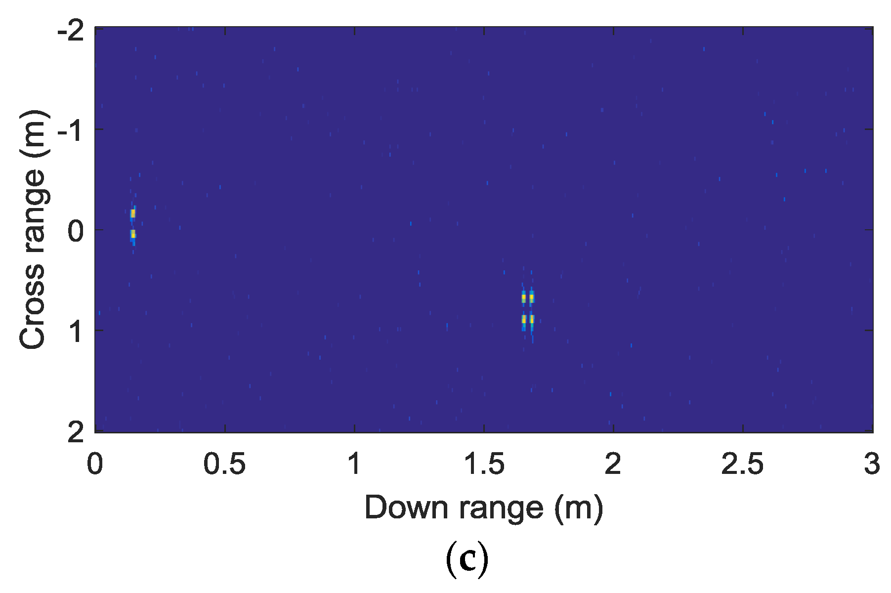
Firstly, an indoor experiment was conducted on a concrete wall inside an office, which was 20 cm thick and with random iron bars inside, as shown in Figure 11a. As previously mentioned, we obtain the number of objects, namely, the value of M, through the algorithm MDL. The estimated values of M by 100 repeated detection trials are shown in Figure 11b. The water target, four identical square blocks, each with 20 cm side lengths, are arranged in the position 2 m away from the wall with azimuth 30°. One frame of the detection results is shown in Figure 11c, which estimates = 5 for water blocks due to large RCS, about 1 m crossrange, and about 1.7 m downrange. Two significant peaks appeared in the 20 cm-range, 0°~3° azimuth angle due to the wall, which can be mitigated or removed according to the previous works in [25,28,29].
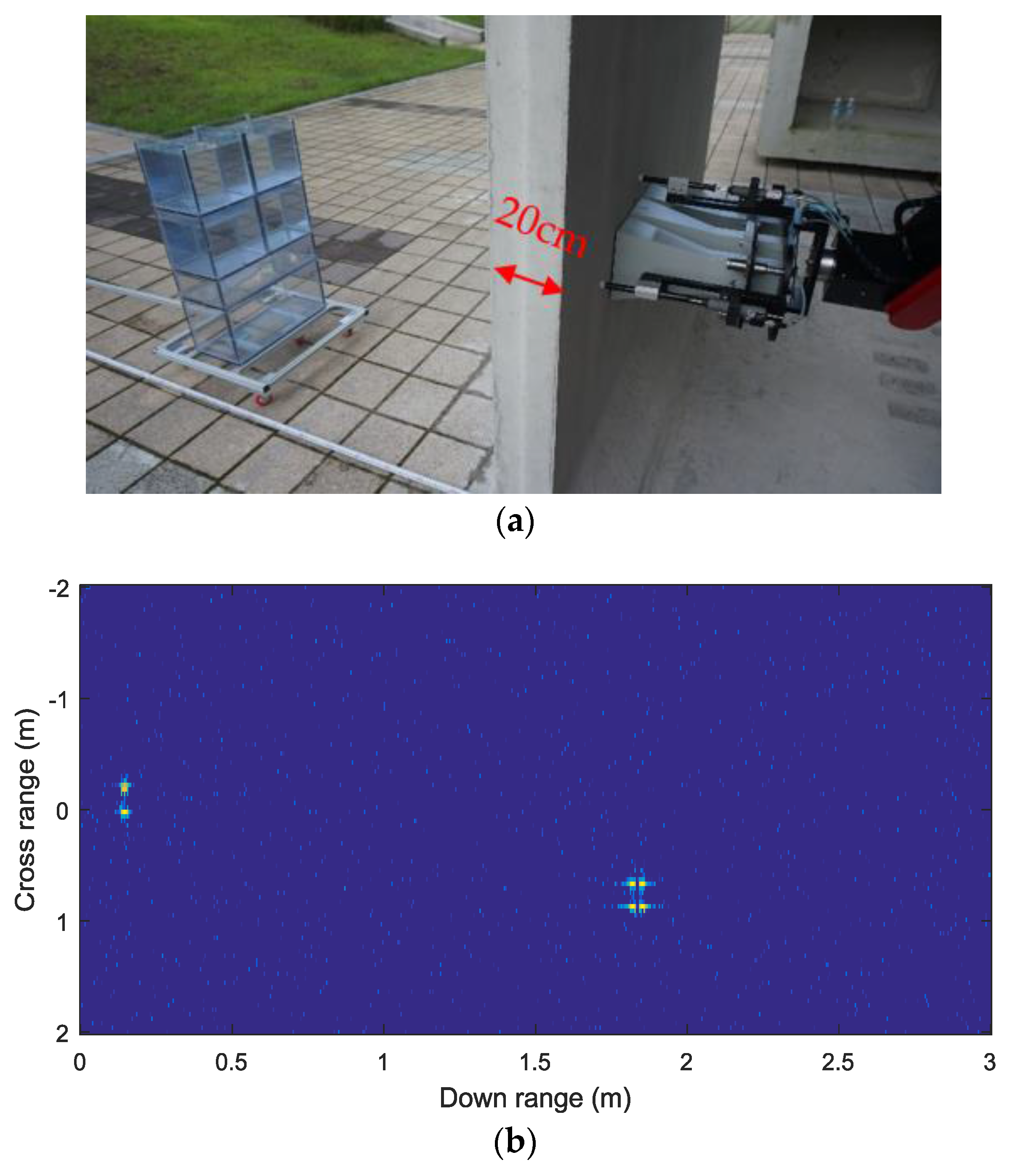
A second set of experiments was carried out inside a concrete block behind an office building. This concrete block was specially made for use in an underground sewage system, one side is also 20 cm thick and contains embedded iron bars. Two experiments were organized by detecting the water blocks and an adult man moving away from the radar with a radial speed of 1 m/s, respectively. Figure 12a shows the whole TWRI system where the front-end module is placed in one concrete block, with iron bars inside the wall. The results of detecting the moving water blocks are displayed, and one frame of the results is shown in Figure 12b. The result shown in Figure 12b indicates that the position of peak is crossrange 1 m, and downrange 1.8 m, which means that the azimuth angle is about 29°. The range-Doppler map corresponding to the frame of Figure 12b is shown in Figure 12c which displays the straight-line range about 2.1 m and the Doppler frequency of about −25 Hz of the targets. The wall targets were shown as the zero Doppler components in the range-Doppler map.
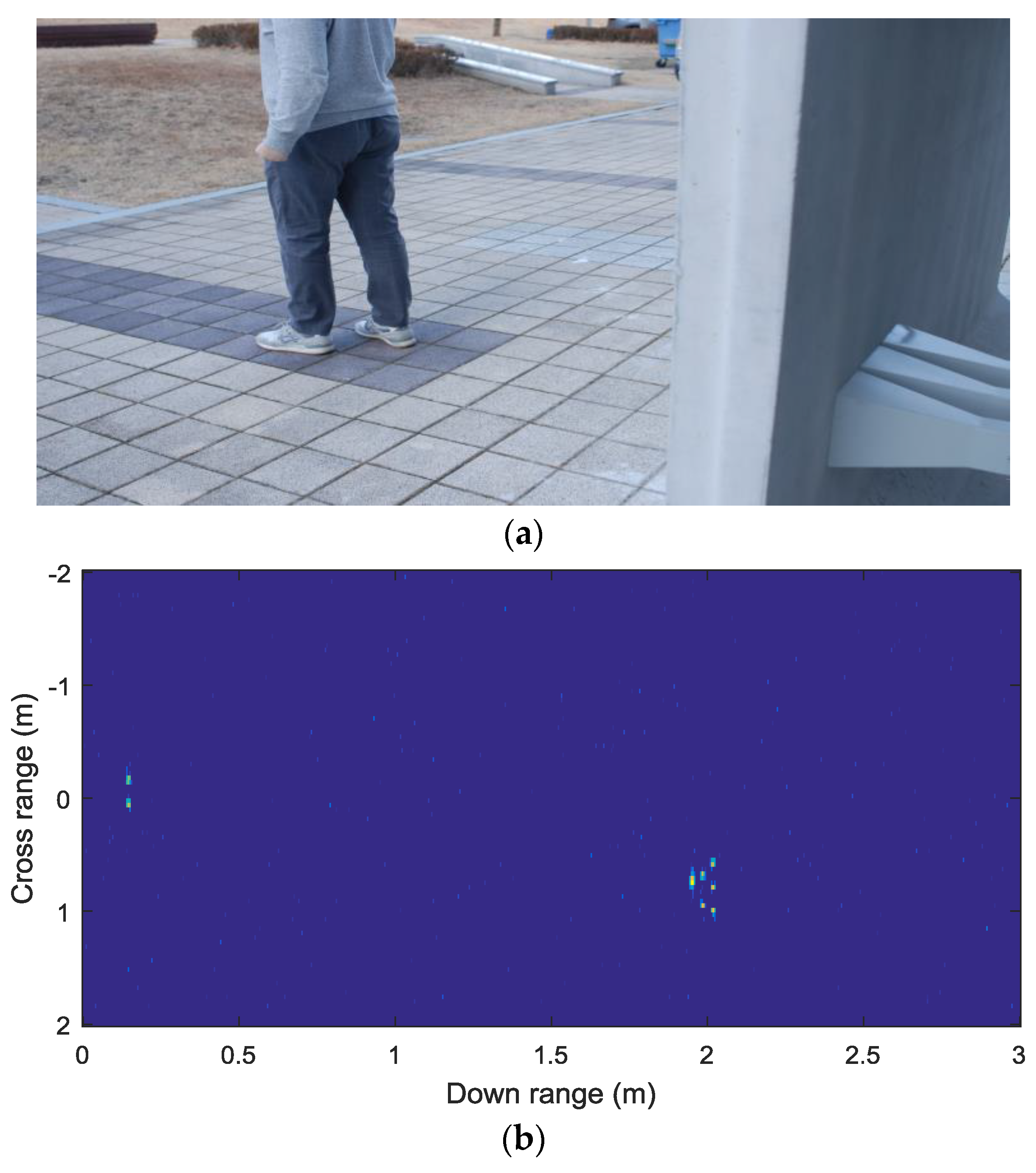
For the experiment with a person target, the adult man was moving away from the wall, as shown in Figure 13a. One frame of the detection results is shown in Figure 13b, which estimates = 8 for human body, and the azimuth angle is about 27° with about 1 m crossrange, and about 2 m downrange. Figure 13c shows the corresponding frame of results, which displays the straight-line range about 2.2 m and Doppler frequency of about −25 Hz. The main components of a human, which reflect incoming RF signals, are head, arms, body, and legs as reported in [16]. Thus, it can be observed that more than five peaks were obtained in Figure 13b, corresponding to the main components of humans. Since the two receiving channels are placed in a horizontal direction, the elevation angle of human components is not considered in the suggested TWRI system, resulting in the peak pattern not like that of a human shown in Figure 13b,c.
6. Conclusions
This paper has presented a dual channel S-Band FMCW system for through-wall radar imaging and proposed the range-angle-Doppler 3D estimation algorithm based on the 3D shift invariant structure. Our experimental results demonstrated that the implemented TWRI system with the proposed algorithm achieved high quality when imaging targets behind concrete walls. However, the proposed algorithm, comprising a variety of matrix operations such as SVD, is not implemented in FPGA and DSP but rather operated in MATLAB on a PC due to the large operating costs. A study on a low complexity version of the suggested algorithm would be needed to implement a real-time TWRI system with two receiving channels.
Acknowledgments
This work was supported by the DGIST R&D Program of the Ministry of Science and ICT(17-ST-01), and this work was supported by the DGIST R&D Program of the Ministry of Science and ICT(17-IT-03).
Author Contributions
All authors conceived and designed the system and experiments together; Ying-chun Li and Daegun Oh performed the experiments and analyzed the data. Daegun Oh was the lead developer for the hardware used and contributed to the experiments work. Sunwoo Kim and Chong-Wha Jong contributed analysis tools/evaluation of system.
Conflicts of Interest
Authors declare no conflict of interest.
References
- Charvat, G.L.; Kempel, L.C.; Rothwell, E.J.; Coleman, C.M.; Mokole, E.L. A through-dielectric radar imaging system. IEEE Trans. Antennas Propag. 2010, 58, 2594–2603. [Google Scholar] [CrossRef]
- Qian, J.; Ahmad, F.; Amin, M.G. Joint localization of stationary and moving targets behind walls using sparse scene recovery. J. Electron. Imaging 2013, 22. [Google Scholar] [CrossRef]
- Amin, M.G. Through-The-Wall Radar Imaging; CRC Press: Boca Raton, FL, USA, 2010. [Google Scholar]
- Gennarelli, G.; Ludeno, G.; Soldovieri, F. Real-Time Through-Wall Situation Awareness Using a Microwave Doppler Radar Sensor. Remote Sens. 2016, 8, 621. [Google Scholar] [CrossRef]
- Yoon, Y.S.; Amin, M.G. Spatial Filtering for Wall-Clutter Mitigation in Through-the-Wall Radar Imaging. IEEE Trans. Geosci. Remote Sens. 2009, 47, 3192–3208. [Google Scholar] [CrossRef]
- Liu, J.; Kong, L.; Yang, X.; Liu, Q.H. Refraction Angle Approximation Algorithm for Wall Compensation in TWRI. IEEE Geosci. Remote Sens. Lett. 2016, 13, 943–946. [Google Scholar] [CrossRef]
- Debes, C.; Zoubir, A.M.; Amin, M.G. Enhanced Detection Using Target Polarization Signatures in Through-the-Wall Radar Imaging. IEEE Trans. Geosci. Remote Sens. 2012, 50, 1968–1979. [Google Scholar] [CrossRef]
- Sachs, J.; Aftanas, M.; Crabbe, S.; Drutarovsky, M.; Klukas, R.; Kocur, D.; Nguyen, T.T.; Peyerl, P.; Rovnakova, J.; Zaikov, E. Detection and tracking of moving or trapped people hidden by obstacles using ultrawideband pseudo-noise radar. In Proceedings of the 2008 European Radar Conference (EuRAD), Amsterdam, The Netherlands, 30–31 October 2008; pp. 408–411. [Google Scholar]
- Browne, K.E.; Burkholder, R.J.; Volakis, J.L. Through-wall opportunistic sensing system utilizing a low-cost flat-panel array. IEEE Trans. Antennas Propag. 2011, 59, 859–868. [Google Scholar] [CrossRef]
- Biying, L.; Song, Q.; Zhou, Z.; Wang, H. A SFCW radar for through wall imaging and motion detection. In Proceedings of the European Radar Conference (EuRAD), Manchester, UK, 12–14 October 2011; pp. 325–328. [Google Scholar]
- Biying, L.; Song, Q.; Zhou, Z.; Zhang, X. Detection of human beings in motion behind the wall using SAR interferogram. IEEE Geosci. Remote Sens. Lett. 2012, 9, 968–971. [Google Scholar] [CrossRef]
- Maaref, N.; Millot, P. Array-based UWB FMCW through-the-wall radar. In Proceedings of the 2012 IEEE Antennas and Propagation Society International Symposium (APSURSI), Chicago, IL, USA, 8–14 July 2012; pp. 1–2. [Google Scholar]
- Maaref, N.; Millot, P. Array-based ultrawideband through-wall radar: Prediction and assessment of real radar abilities. Int. J. Antennas Propag. 2013, 2013. [Google Scholar] [CrossRef]
- Charvat, G.L.; Kempel, L.C.; Rothwell, E.J.; Coleman, C.M.; Mokole, E.L. A through-dielectric ultrawideband (UWB) switchedantenna-array radar imaging system. IEEE Trans. Antennas Propag. 2012, 60, 5495–5500. [Google Scholar] [CrossRef]
- Ralston, T.S.; Charvat, G.L.; Peabody, J.E. Real-time through-wall imaging using an ultrawideband multiple-input multiple-output (MIMO) phased array radar system. In Proceedings of the IEEE International Symposium on Phased Array Systems and Technology (ARRAY 2010), Waltham, MA, USA, 12–15 October 2010; pp. 551–558. [Google Scholar]
- Peabody, J.; Charvat, G.L.; Goodwin, J.; Tobias, M. Through-Wall Imaging Radar. Linc. Lab. J. 2012, 19, 62–72. [Google Scholar]
- Ahmad, F.; Amin, M.G. Through-the-wall radar imaging experiments. In Proceedings of the IEEE Workshop on Signal Processing Applications for Public Safety and Forensics, Washington, DC, USA, 11–13 April 2007; pp. 132–136. [Google Scholar]
- Hantscher, S.; Reisenzahn, A.; Diskus, C.G. An UWB wall scanner based on a shape estimating SAR algorithm. In Proceedings of the IEEE/MTT-S Microwave Symposium, Honolulu, HI, USA, 3–8 June 2007; pp. 1458–1461. [Google Scholar]
- Hantscher, S.; Praher, B.; Reisenzahm, A.; Diskus, C.G. 2D imaging algorithm for the evaluation of UWB B-Scans. In Proceedings of the IEEE Conference on Ultrawideband and Ultrashort Impulse Signals, Sevastopol, Ukraine, 18–22 September 2006; pp. 139–141. [Google Scholar]
- Thajudeen, C.; Hoorfar, A. A Hybrid Bistatic–Monostatic Radar Technique for Calibration-Free Estimation of Lossy Wall Parameters. IEEE Antennas Wirel. Propag. Lett. 2017, 16, 1249–1252. [Google Scholar] [CrossRef]
- Lang, S.A.; Demming, M.; Jaeschke, T.; Noujeim, K.M.; Konynenberg, A.; Pohl, N. 3D SAR imaging for dry wall inspection using an 80 GHz FMCW radar with 25 GHz bandwidth. In Proceedings of the 2015 IEEE MTT-S International Microwave Symposium, Phoenix, AZ, USA, 17–22 May 2015; pp. 1–4. [Google Scholar] [CrossRef]
- Sevigny, P.; DiFilippo, D.J.; Laneve, T.; Fournier, J. Indoor imagery with a 3D through-wall synthetic aperture radar. In Proceedings of the SPIE 8361, Radar Sensor Technology XVI, Baltimore, MD, USA, 4 May 2012; pp. 1–7. [Google Scholar] [CrossRef]
- Amin, M.G.; Ahmad, F. Wideband synthetic aperture beamforming for through-the-wall imaging [Lecture Notes]. IEEE Signal Process. Mag. 2008, 25, 110–113. [Google Scholar] [CrossRef]
- Seng, C.H.; Amin, M.G.; Ahmad, F.; Bouzerdoum, A. Image Segmentations for Through-the-Wall Radar Target Detection. IEEE Trans. Aerosp. Electron. Syst. 2013, 49, 1869–1896. [Google Scholar] [CrossRef]
- Leigsnering, M.; Ahmad, F.; Amin, M.G.; Zoubir, A.M. CS based wall ringing and reverberation mitigation for through-the-wall radar imaging. In Proceedings of the 2013 IEEE Radar Conference (RadarCon13), Ottawa, ON, USA, 29 April–3 May 2013; pp. 1–5. [Google Scholar] [CrossRef]
- Leigsnering, M.; Ahmad, F.; Amin, M.; Zoubir, A. Multipath exploitation in through-the-wall radar imaging using sparse reconstruction. IEEE Trans. Aerosp. Electron. Syst. 2014, 50, 920–939. [Google Scholar] [CrossRef]
- Winkler, V. Range Doppler detection for automotive FMCW radars. In Proceedings of the 2007 European Radar Conference, Munich, Germany, 10–12 October 2007; pp. 166–169. [Google Scholar] [CrossRef]
- Tivive, F.H.C.; Bouzerdoum, A. An improved SVD-based wall clutter mitigation method for through-the-wall radar imaging. In Proceedings of the 2013 IEEE 14th Workshop on Signal Processing Advances in Wireless Communications (SPAWC), Darmstadt, Germany, 16–19 June 2013; pp. 430–434. [Google Scholar] [CrossRef]
- Tivive, F.H.C.; Bouzerdoum, A.; Amin, M.G. A Subspace Projection Approach for Wall Clutter Mitigation in Through-the-Wall Radar Imaging. IEEE Trans. Geosci. Remote Sens. 2015, 53, 2108–2122. [Google Scholar] [CrossRef]
- Meta, A. Signal Processing of FMCW Synthetic Aperture Radar Data. Available online: http://resolver.tudelft.nl/uuid:24352ff9-c11a-46c9-87d4-4d9d8968ed81 (accessed on 10 August 2017).
- Dehmollaian, M.; Thiel, M.; Sarabandi, K. Through-the-Wall Imaging Using Differential SAR. IEEE Trans. Geosci. Remote Sens. 2009, 47, 1289–1296. [Google Scholar] [CrossRef]
- Li, G.; Burkholder, R.J. Hybrid matching pursuit for distributed through-wall radar imaging. IEEE Trans. Antennas Propag. 2015, 63, 1701–1711. [Google Scholar] [CrossRef]
- Ahmad, F.; Amin, M.G.; Kassam, S.A. Synthetic aperture beamformer for imaging through a dielectric wall. IEEE Trans. Aerosp. Electron. Syst. 2005, 41, 271–283. [Google Scholar] [CrossRef]
- Hua, Y.; Sarkar, T.K. Matrix pencil method for estimating parameters of exponentially damped/undamped sinusoids in noise. IEEE Trans. Acoust. Speech Signal Process. 1990, 38, 814–824. [Google Scholar] [CrossRef]
- Wax, M.; Kailath, T. Detection of signals by information theoretic criteria. IEEE Trans. Acoust. Speech Signal Process. 1985, ASSP-33, 387–392. [Google Scholar] [CrossRef]
- Oh, D.; Lee, J. Robust Super-Resolution TOA Estimation against Doppler Shift for Vehicle Tracking. IEEE Commun. Lett. 2014, 18, 745–748. [Google Scholar] [CrossRef]
Figure 1.
Geometry of TWRI system, (a) practical models of wave propagation, (b) simplified model for proposed algorithm.
Figure 1.
Geometry of TWRI system, (a) practical models of wave propagation, (b) simplified model for proposed algorithm.

Figure 2.
Illustration of high-pass filtering, (a) Beat signals before filtering, (b) Filtered beat signals.
Figure 2.
Illustration of high-pass filtering, (a) Beat signals before filtering, (b) Filtered beat signals.

Figure 3.
TWRI SAR geometry in [31].
Figure 3.
TWRI SAR geometry in [31].

Figure 4.
3D Shift Invariant Structure.
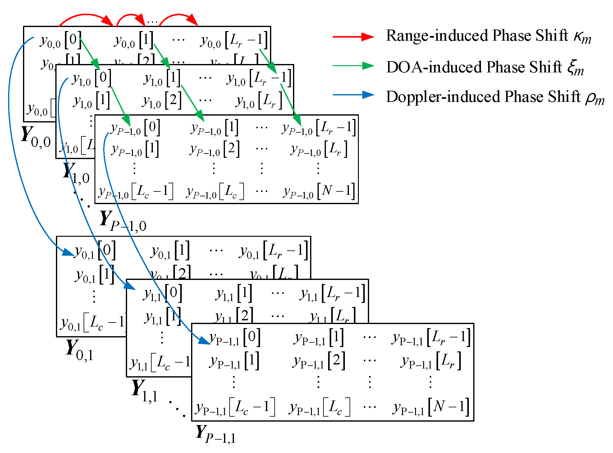
Figure 5.
Block diagram of the S-Band FMCW TWRI radar system.

Figure 6.
Bandpass filter (a) Image of real product (b) Filter response.
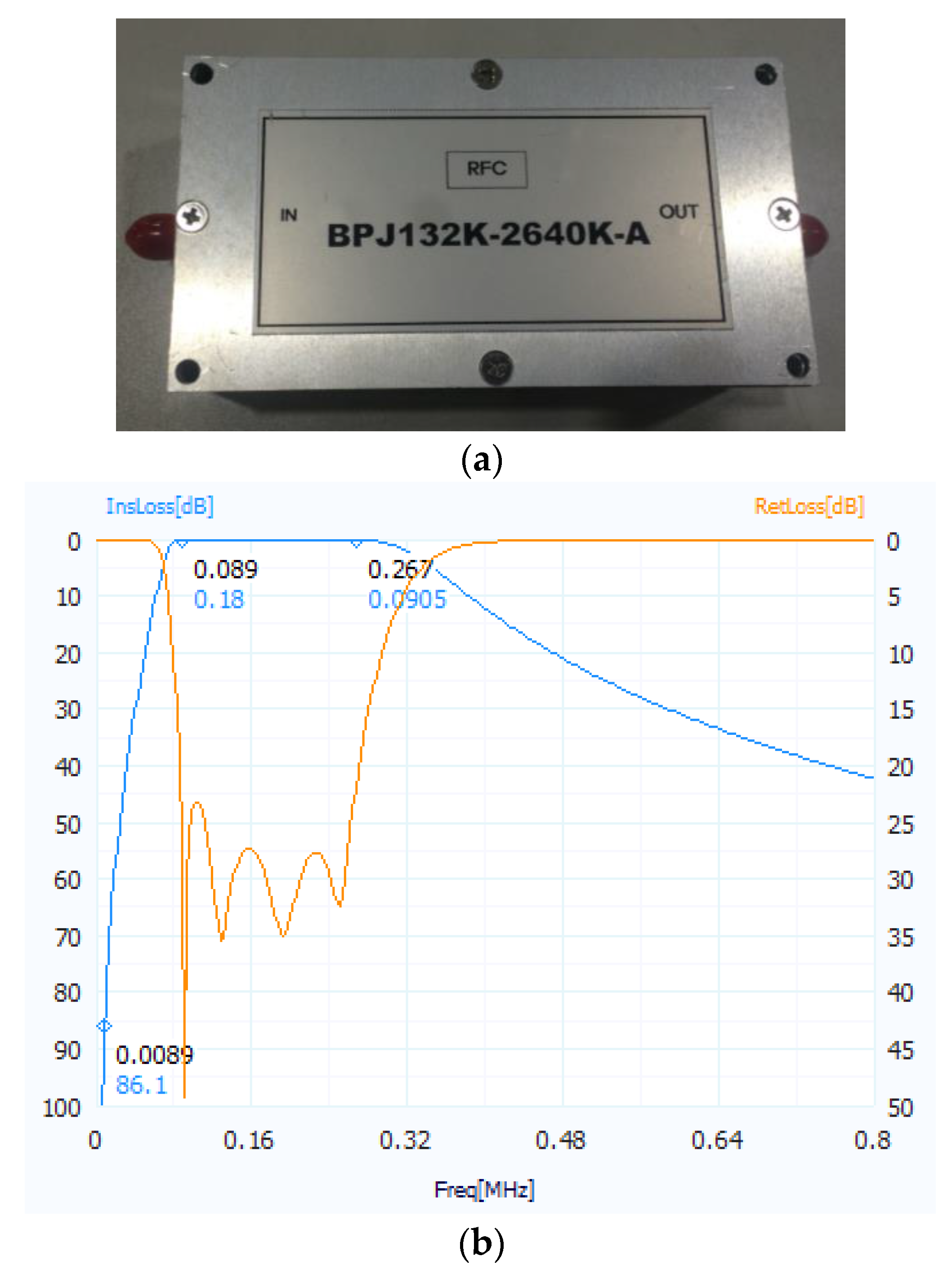
Figure 7.
(a) Standard horn antenna. (b) Antenna array. (c) Pattern at 3 GHz, H-plane with 3 dB beam width 43.51° and E-plane pattern with 3 dB beam width 51.32°.
Figure 7.
(a) Standard horn antenna. (b) Antenna array. (c) Pattern at 3 GHz, H-plane with 3 dB beam width 43.51° and E-plane pattern with 3 dB beam width 51.32°.

Figure 8.
Outward appearance of implemented S-band FMCW TWRI radar system.

Figure 9.
Inward appearance of implemented S-band FMCW TWRI radar system.
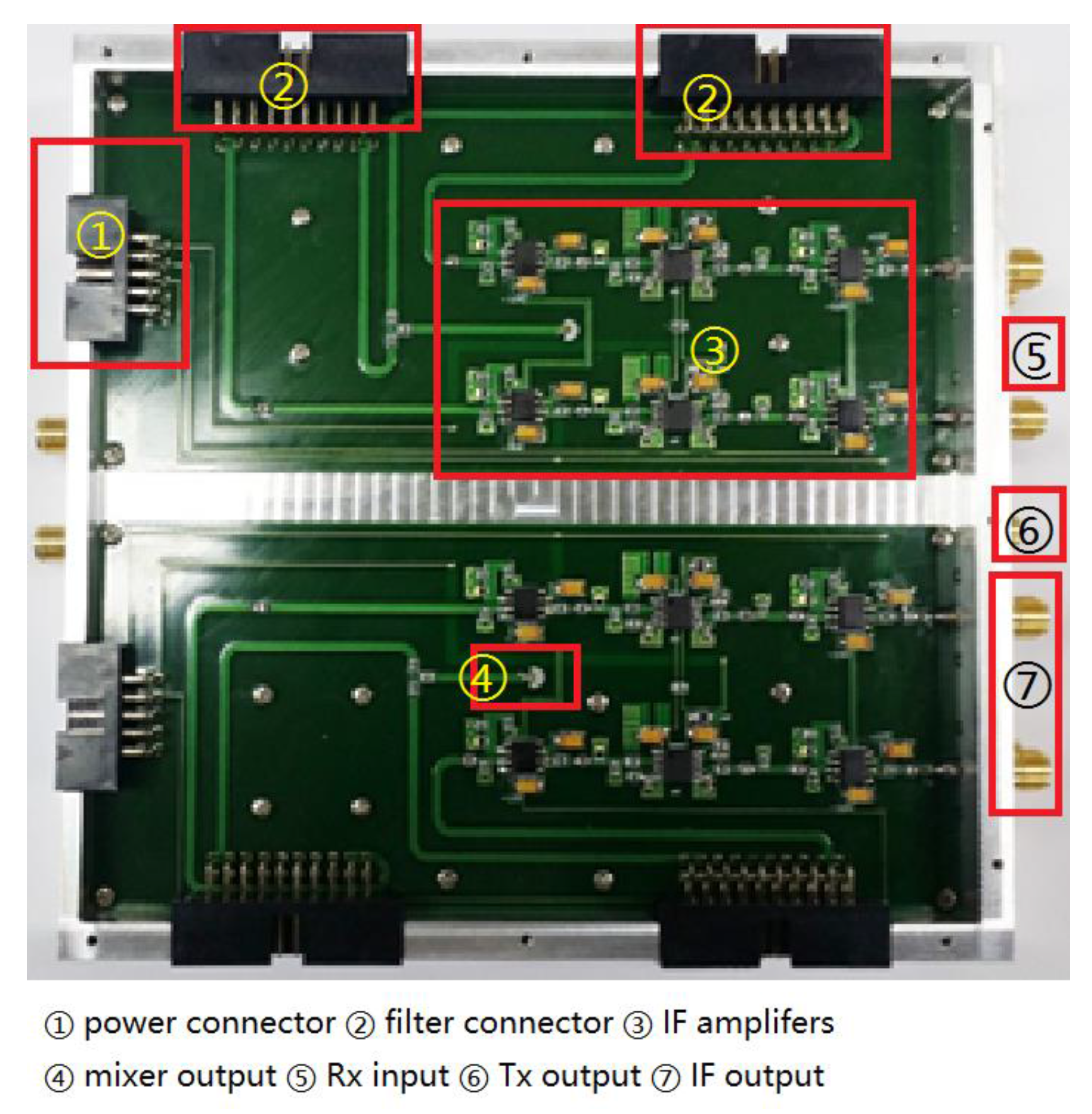
Figure 10.
FPGA and DSP board.
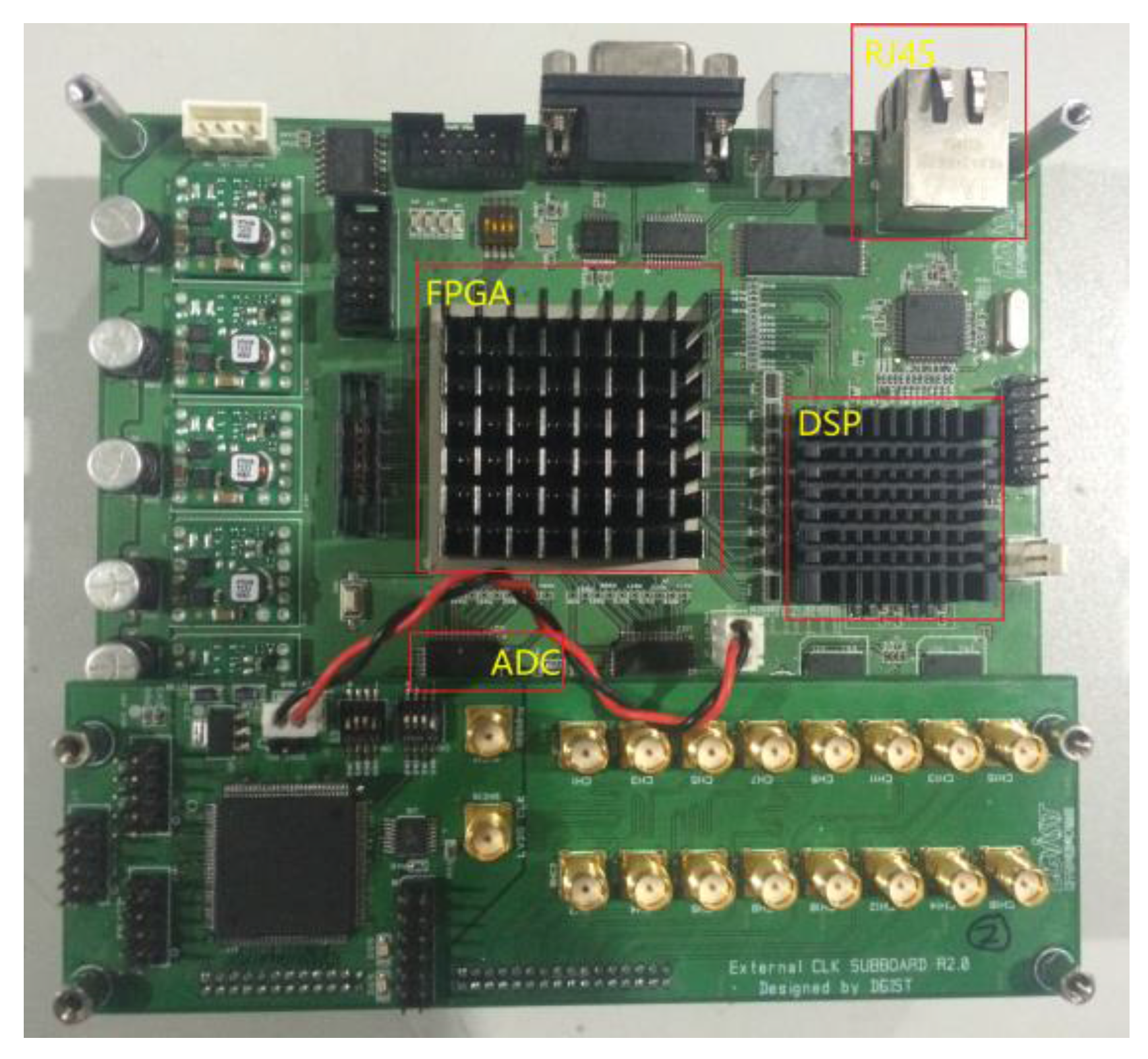
Figure 11.
(a) Imaged indoor scene, (b) Value of M obtained by MDL through 100 experiment trials; (c) One frame of the detection results obtained when = 6.
Figure 11.
(a) Imaged indoor scene, (b) Value of M obtained by MDL through 100 experiment trials; (c) One frame of the detection results obtained when = 6.
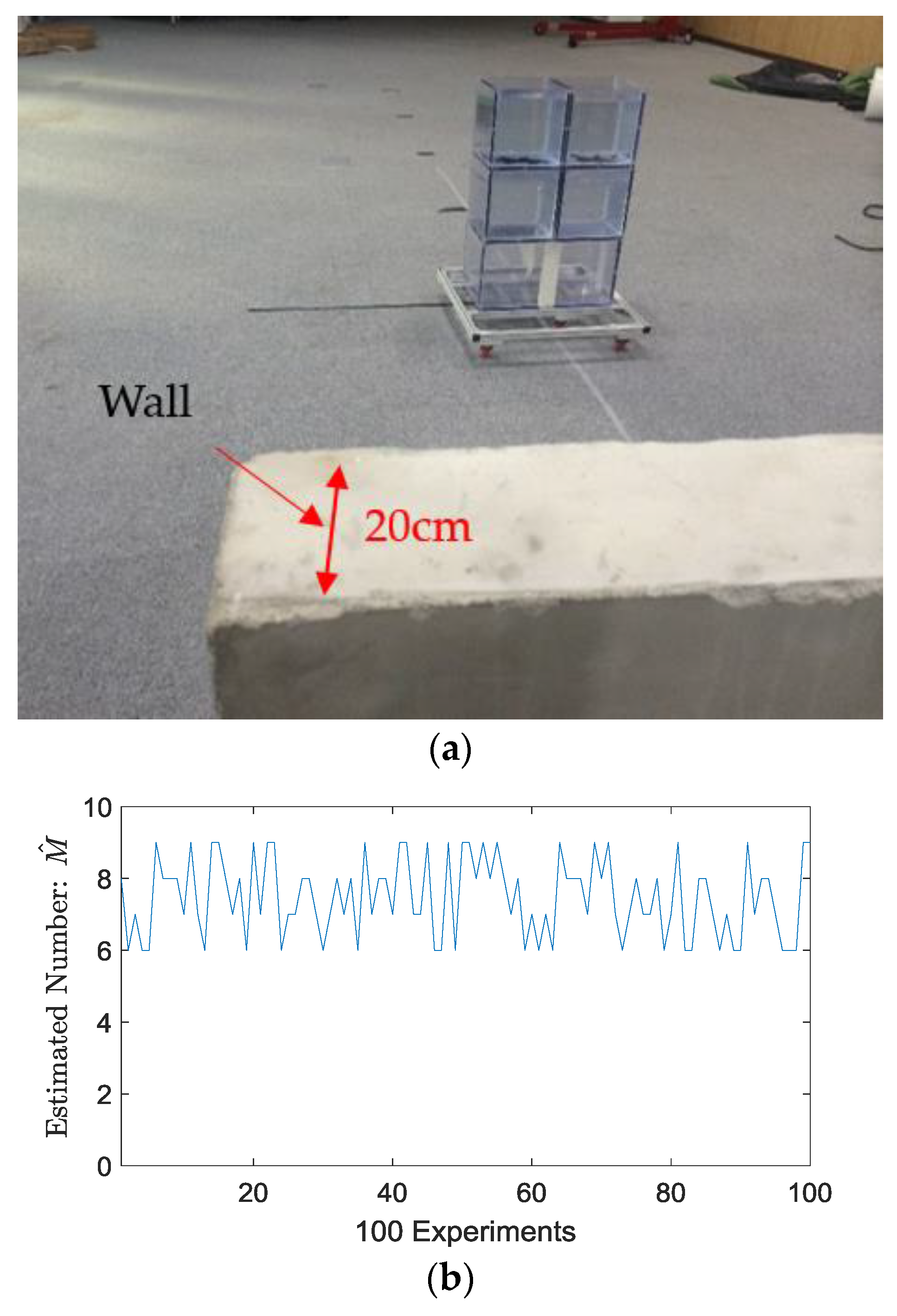

Figure 12.
(a) Imaged outdoor scene; water target and TWRI system. (b) One frame of detection results of multi targets (water blocks) behind the wall when = 5. (c) One frame of Range-Doppler maps, showing the Doppler frequency.
Figure 12.
(a) Imaged outdoor scene; water target and TWRI system. (b) One frame of detection results of multi targets (water blocks) behind the wall when = 5. (c) One frame of Range-Doppler maps, showing the Doppler frequency.

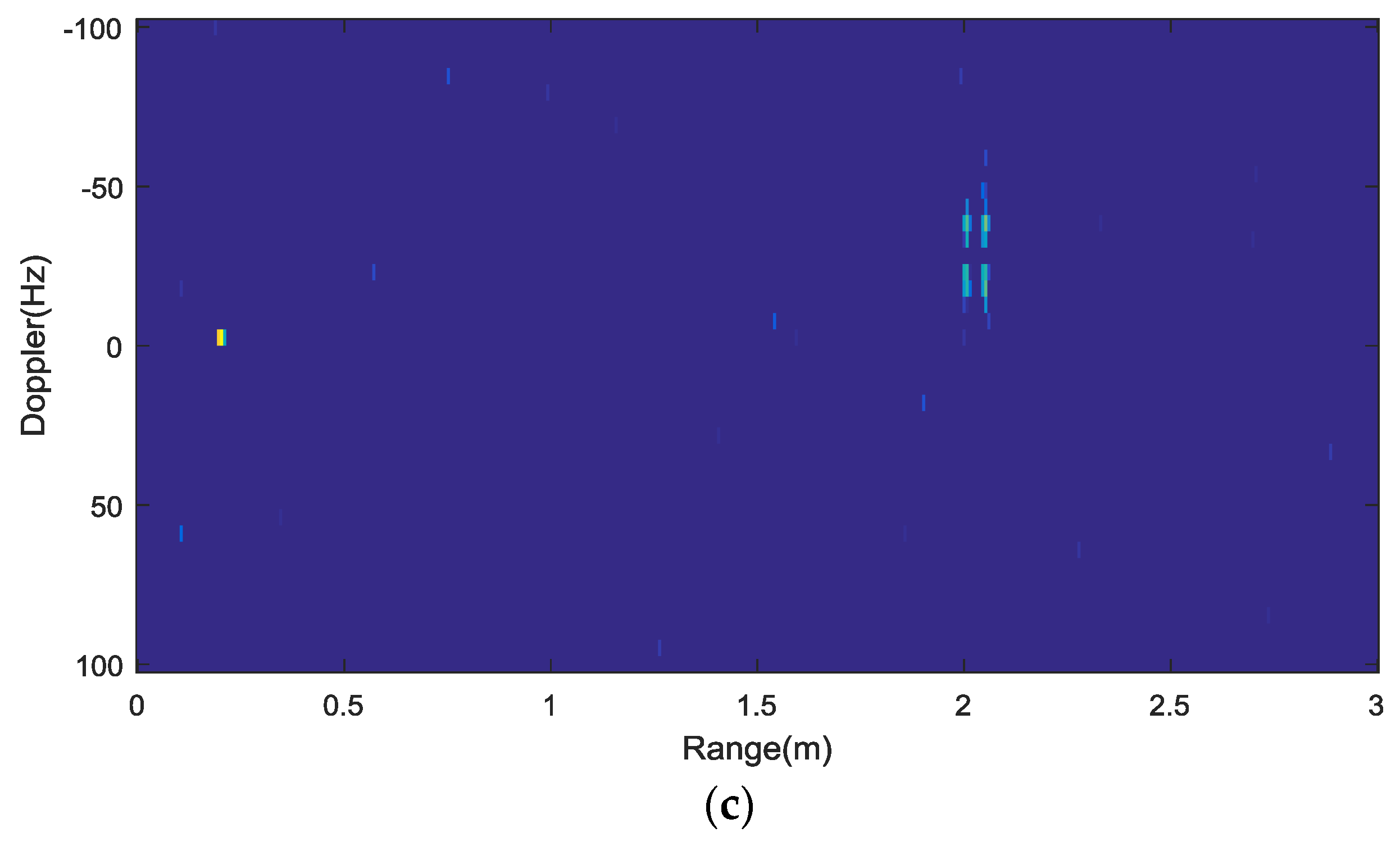
Figure 13.
(a) Imaged scene for person detection. (b) One frame of the detection results when = 8. (c) One frame of Range-Doppler maps, showing the Doppler frequency.
Figure 13.
(a) Imaged scene for person detection. (b) One frame of the detection results when = 8. (c) One frame of Range-Doppler maps, showing the Doppler frequency.


Table 1.
Summary of System Specifications.
| Parameter | Specification |
|---|---|
| Modulation type | FMCW |
| Receiver | I & Q demodulation |
| Receiver dynamic range | 72 dB |
| Carrier frequency | 2.9 GHz |
| Bandwidth | 600 MHz |
| Peak power | 1 W |
| Velocity resolution | 25 Hz |
| Range resolution | 25 cm |
| Tx and Rx antenna | Standard horn antenna |
© 2018 by the authors. Licensee MDPI, Basel, Switzerland. This article is an open access article distributed under the terms and conditions of the Creative Commons Attribution (CC BY) license (http://creativecommons.org/licenses/by/4.0/).
Share and Cite
MDPI and ACS Style
Li, Y.-C.; Oh, D.; Kim, S.; Chong, J.-W. Dual Channel S-Band Frequency Modulated Continuous Wave Through-Wall Radar Imaging. Sensors 2018, 18, 311. https://doi.org/10.3390/s18010311
AMA Style
Li Y-C, Oh D, Kim S, Chong J-W. Dual Channel S-Band Frequency Modulated Continuous Wave Through-Wall Radar Imaging. Sensors. 2018; 18(1):311. https://doi.org/10.3390/s18010311
Chicago/Turabian StyleLi, Ying-Chun, Daegun Oh, Sunwoo Kim, and Jong-Wha Chong. 2018. "Dual Channel S-Band Frequency Modulated Continuous Wave Through-Wall Radar Imaging" Sensors 18, no. 1: 311. https://doi.org/10.3390/s18010311
Note that from the first issue of 2016, this journal uses article numbers instead of page numbers. See further details here.