G-Networks to Predict the Outcome of Sensing of Toxicity


1
University Côte d’Azur, I3S laboratory, UMR CNRS 7271, CS 40121, 06903 Sophia Antipolis CEDEX, France
2
Intelligent Systems and Networks Group, Department of Electrical and Electronic Engineering, Imperial College, London SW7 2AZ, UK
*
Author to whom correspondence should be addressed.
Sensors 2018, 18(10), 3483; https://doi.org/10.3390/s18103483
Submission received: 14 August 2018
/
Revised: 5 October 2018
/
Accepted: 12 October 2018
/
Published: 16 October 2018
(This article belongs to the Special Issue G-Networks for Security, Low Energy Consumption and Quality of Service of the Internet of Things)
Abstract
:G-Networks and their simplified version known as the Random Neural Network have often been used to classify data. In this paper, we present a use of the Random Neural Network to the early detection of potential of toxicity chemical compounds through the prediction of their bioactivity from the compounds’ physico-chemical structure, and propose that it be automated using machine learning (ML) techniques. Specifically the Random Neural Network is shown to be an effective analytical tool to this effect, and the approach is illustrated and compared with several ML techniques.
1. Introduction
G-Networks [1] are a family of queueing networks with a convenient and computationally efficient product form mathematical solution. The computation of the state of a G-Network is obtained via a simple fixed-point iteration, and the existence and uniqueness of the solution to the key G-Network state equation is easily verified [2]. G-Networks incorporate useful primitives, such as the transfer of jobs between servers or the removal of batches of jobs from excessively busy servers, which were developed in several successive papers including [3,4,5,6].
They have a wealth of diverse applications as a tool to analyse and optimise the effects of dynamic load balancing in large scale networks and distributed computer systems [7]. They are also used to model Gene Regulatory Networks [8,9]. A recent application of G-Networks is to the modelling of systems which operate with intermittent sources of energy, known as Energy Packet Networks [10,11,12,13,14,15].
The simplest version of G-Networks, known as the Random Neural Network (RNN) [16], has a powerful property of approximating continuous and bounded real-valued functions [17]. This property serves as the foundation for RNN based learning algorithms [18] and Deep Learning [19,20].
The RNN has been used for modelling natural neuronal networks [21], and for protein alignment [22]. It has been used with its learning algorithm [18] in several image processing applications including learning colour textures [23], the accurate evaluation of tumours from brain MRI scans [24] and the compression of still and moving images [25,26,27]. It was recently introduced as a tool for predicting the toxicity of chemical compounds [28].
In the field of computer network performance, the RNN has been used to build distributed controllers for quality of service routing in packet networks [29,30,31] and in the design of Software Defined Network controllers for the Internet [32,33]. Real-time optimised task allocation algorithms in Cloud systems [34,35] have also been built and tested. Recent applications have addressed the use of the RNN to detect network attacks [36] and attacks on Internet of Things (IoT) gateways [37].
In this paper, we introduce the use of the RNN and other ML techniques to reduce the use of in vivo laboratory experiments in the evaluation of the bioactivity and potential toxicity of chemical compounds. Indeed, the hope is that the toxicity of chemical compounds may in the future be determined through physical-chemical-computational means and processes, avoiding the use of laboratory animals.
Prediction in this area is challenging [38,39] because of high biological variability, especially when toxicity is the result from a sequence of causal factors. Therefore, we suggest that long-term toxicity prediction could be obtained by the prediction of in vitro bioactivity using chemical structure [40], followed by the prediction of in vivo effects from in vitro bioactivity [41,42].
Here, we only develop the first part of this challenge based on the RNN and other ML techniques to elucidate the quantitative structure–activity relationship (QSAR) [43] which predicts a compound’s activity using its physico-chemical properties and structural descriptors.
2. RNN Based Learning and Other Methods
Since we need publicly available and agreed upon data in order to train and test the ML methods, including the RNN, we call upon the data released by the US Environmental Protection Agency (EPA) in the ToxCast database (https://www.epa.gov/chemical-research/exploring-toxcast-data, October 2015 release) which contains bioactivity data obtained for around 10,000 of compounds tested in more than several hundreds in vitro assays [44], and the Toxicity Reference database (ToxRefDB) with results from several types of in vivo studies for several hundreds of chemicals [45]. These data sets do not fully cover each other so that not all compounds tested in ToxCast are present in ToxRefDB.
We consider a subset of these data including compounds for which both in vitro and in vivo results are available. The subset selection follows three steps. First, we look for the overlap of compounds present both in ToxCast and ToxRefDB and having results for in vivo studies performed in rats during two years. We obtain a matrix with 418 compounds and 821 assays, with a lot of missing values. Secondly, we look for a large complete sub-matrix and we obtain a matrix of 404 compounds and 60 in vitro assays. Finally, in order to be sure to get a minimum of active compounds in the datasets, i.e., compounds for which an AC50 (half maximal activity concentration) could be measured, we remove assays with less than 5% of them and obtain a final matrix of 404 compounds and 37 assays.
For each of the 37 assays, we build a QSAR classification model to predict the bioactivity of a compound. These models use structural descriptors computed from the compound’s structure described in Structured Data Files. Two types of descriptors are used: (i) 74 physico-chemical properties (e.g., molecular weight, logP, etc.), which are continuous variables calculated using the RDKit Open-Source software [46] and normalized into the interval [0; 1] and (ii) 4870 fingerprints which are binary vectors representing the presence or absence of a chemical sub-structure in a compound [47]. The different types of fingerprints were generated using the pybel package in Python [48] and the PaDEL sofware [49] and are the following: FP3, Estate, KlekotaRoth, MACCS and PubChem fingerprints. Fingerprints being present in less than 5% of compounds are removed, leading to a final set of 731 fingerprints. Therefore, the obtained dataset is composed of 805 structural descriptors for the 404 compounds.
The property that we wish to predict, is the activity in each in vitro assay in a binarised form. It is generally measured as a AC50 value which is the dose of compound required to obtain 50% of activity in the assay. For compounds that were inactive in the assays, meaning that no AC50 could have been determined, an AC50 value of 1,000,000 mM have been used. In the following, we consider that the binary version of the activity is 0 for AC50 of 1,000,000 (meaning inactivity of the compound) and 1 otherwise.
2.1. Learning Algorithms
We recall that The Random Neural Network (RNN) is a simple version of the mathematical models called G-Networks, and that it represents the spiking (impulse-like) probabilistic behaviour of biological neural systems [50] which is a universal approximator for continuous and bounded functions [17]. It has a compact computationally efficient “product form solution”, so that, in steady-state, the joint probability distribution of the states of the neurons in the network can be expressed as the product of the marginal probabilities for each neuron. The probability that any cell is excited satisfies a nonlinear continuous function of the states of the other cells, and it depends on the firing rates of the other cells and the synaptic weights between cells. The RNN has been applied to many pattern analysis and classification tasks [26]. Gradient descent learning is often used for the RNN, but in this work we determine weights of the RNN using the cross-validation approach in [51].
The Multi Layer RNN (MLRNN) uses the original simpler structure of the RNN and investigates the power of single cells for deep learning [20]. It achieves comparable or better classification at much lower computation cost than conventional deep learning methods in some applications. A cross-validation approach is used to determine the structure and the weights and 20 trials are conducted to average the results. The structure of the MLRNN used here is fixed as having 20 inputs and 100 intermediate nodes.
Boosted Trees (called XGBoost in the sequel) is a popular tree ensemble method. The open-source software library XGBoost [52] provides an easy-to-use tool for implementing boosted trees with gradient boosting [53] and regression trees.
For the RNN and MLRNN we use the algorithms and software developed at Imperial College. For the XGBoost, we use the implementation and software explicitly mentioned in the references.
2.2. Classification Settings and Performance Metrics
For each of the 37 assays, we randomly subdivide the corresponding dataset D into a training set and a testing set . From D, we randomly create 50 instances of and its complementary test set so that, for each instance, . Each of the ML techniques listed above are first trained on each and then tested on . The results we present below are therefore averages over the 50 randomly selected training and testing sets. Since the output of the datasets is either 0 or 1, this is a binary classification problem.
Let TP, FP, TN and FN denote the number of true positives, false positives, true negatives and false negatives, respectively. Then, the performance metrics that we use to evaluate the results are the (), the () and the , denoted for short BA (().
3. Classification Results
In the 37 datasets corresponding to the 37 assays, the ratio between positive and negative compounds varies between and with a mean around . This highlights the unbalanced property of the data in the favor of negative compounds. Here, we test the ML algorithms on these unbalanced data and after balancing using data augmentation.
3.1. Results on Unbalanced Datasets
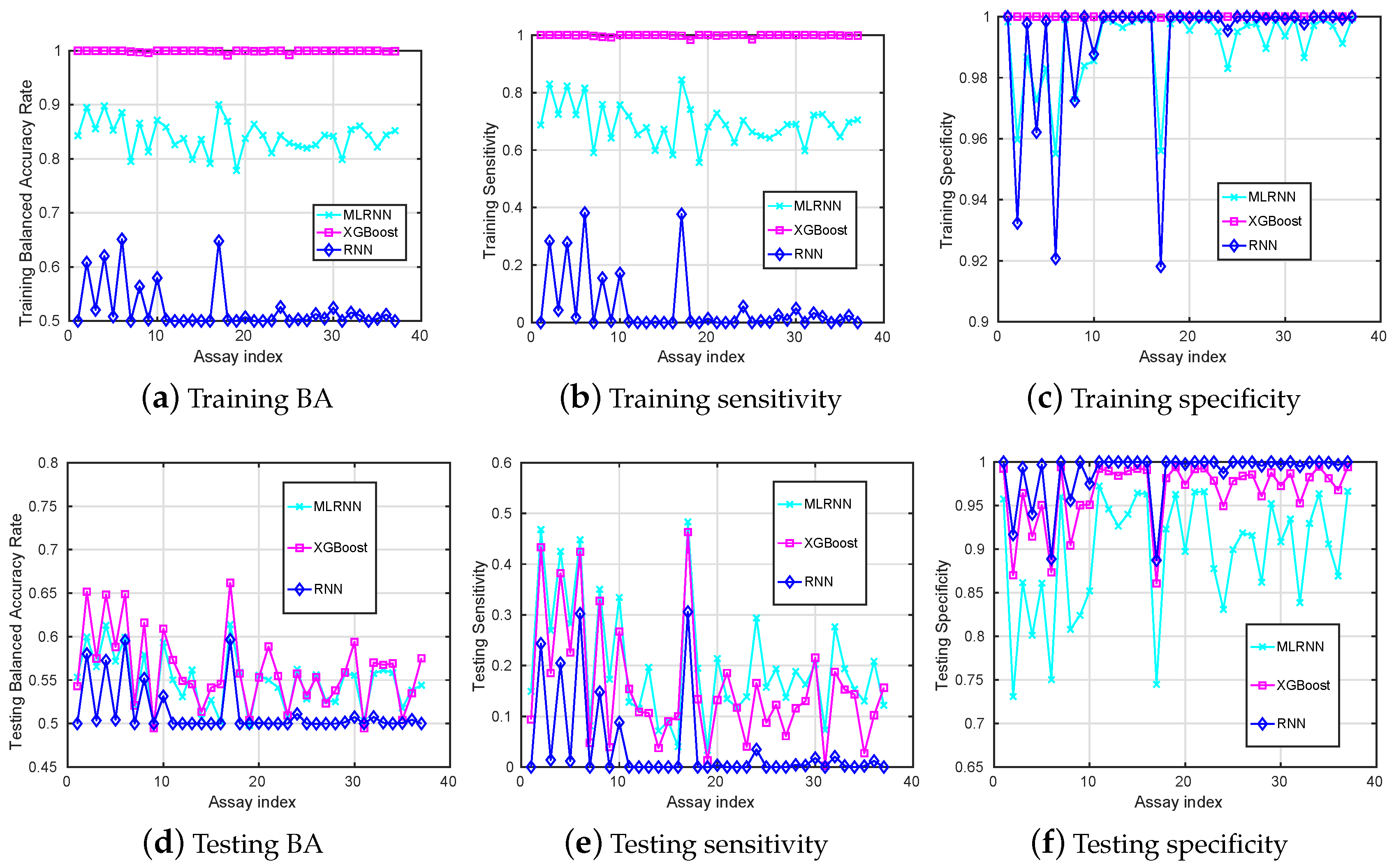
The MLRNN, RNN and XGBoost algorithms are exploited to classify the pairs of training and testing datasets and results are summarized into Figure 1. Since these are unbalanced datasets, the BA may be a better metric to demonstrate the classification accuracy. In addition, the situation of misclassifying positive as negative may be less desirable than that of misclassifying negative as positive. Therefore, the metric of is also important.
When looking at the BA obtained on the training data set in Figure 1a, we observe that the RNN method is not good at learning from these unbalanced datasets, while the MLRNN and XGBoost techniques learn much better.
Compared to the training accuracy, the performance on the testing dataset is more important since it demonstrates whether the model generalises accurately with regard to classifying previously unseen chemical compounds. The testing results are presented in Figure 1d–f. Here, we see that RNN performs the worst in identifying true positives () and tends to classify most unseen chemical compounds as inactive, except for some assays. It can be explained by the overall number of inactive compounds much larger than the number of active compounds in the training dataset. The MLRNN and XGBoost perform a bit better in identifying the TPs, and the MLRNN performs the best. However, is still low and really depends on the assays and probably on the balance between active and inactive compounds in the corresponding datasets.
Among all assays, the highest testing achieved by these classification tools is attained by the XGBoost for assay number 17, with the corresponding being . Among all assays, the highest testing is (MLRNN for assay 17) with a corresponding of .
3.2. Results on Balanced Datasets
From the previous results, it appears that most of the classification techniques used are not good at learning unbalanced datasets. Therefore, we try balancing the training datasets with data augmentation, while the corresponding testing datasets remain unchanged.
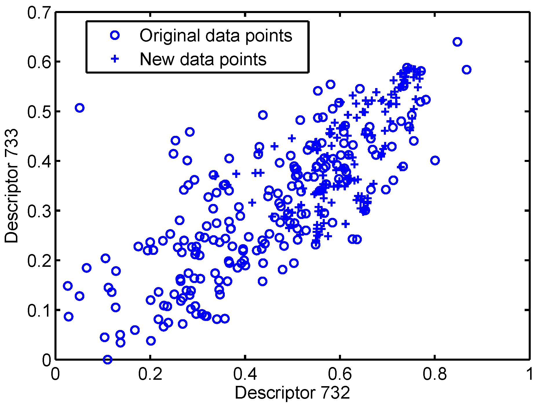
Here, the MLRNN, RNN and XGBoost are used to learn from the datasets which are augmented for balanced training using the SMOTE method [54] as implemented in the Python toolbox unbalanced_learn [55]. Specifically, we plot two descriptors (Descriptors 732 and 733) of the training dataset after data augmentation in Figure 2. We can see that new samples are generated based on the original ones, and added to the dataset. Since the new points are correlated with the existing original points, this could be called “oversampling” (because of the correlation) or “augmentation” because the added points do not exist in the original dataset. The resulting , and are summarised in Figure 3.
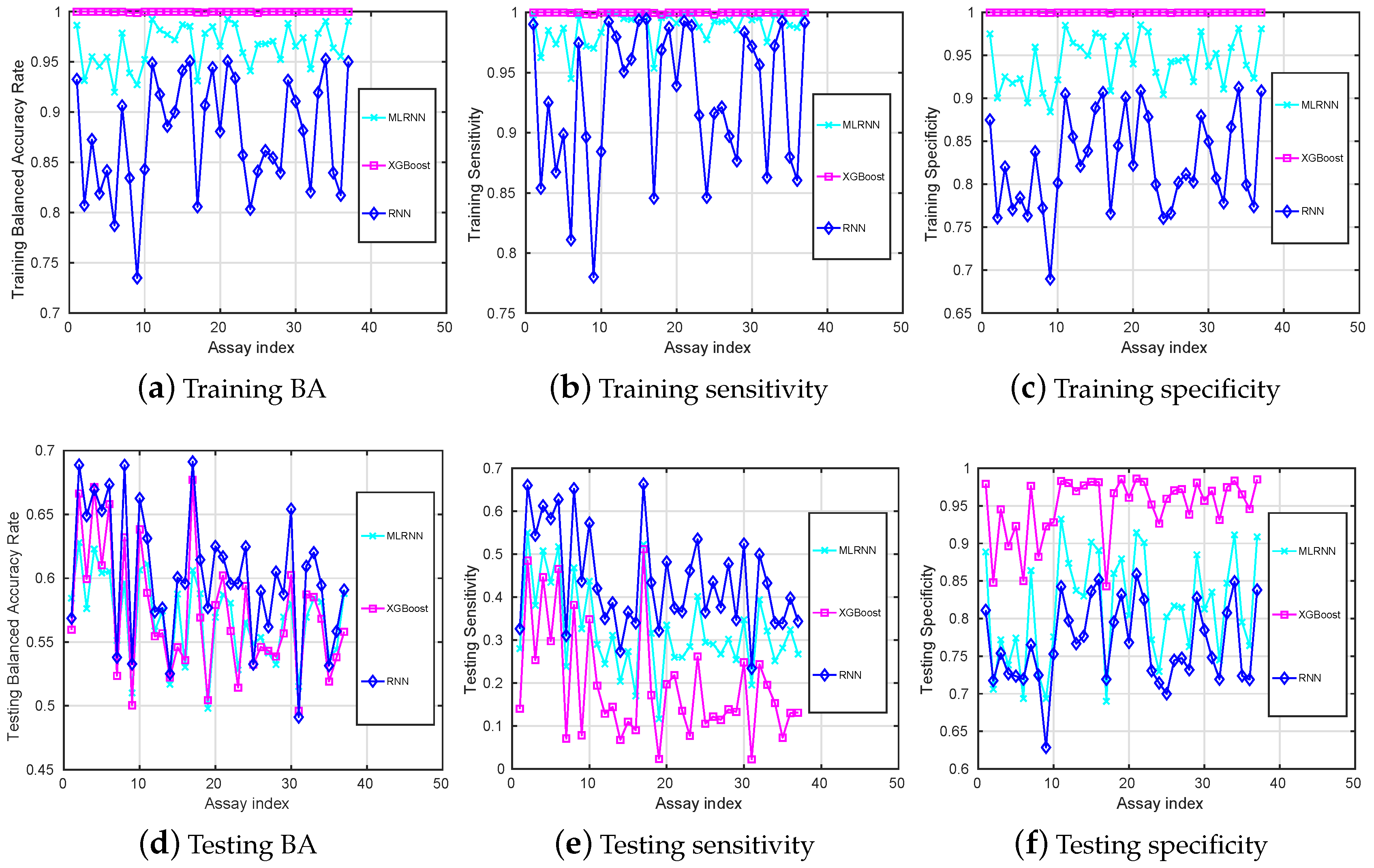
Compared to the training balanced accuracies given in Figure 1a, Figure 3a shows that it is now evident that all the classification techniques we have discussed are capable of learning the training datasets after data augmentation. The training of the RNN method is still the lowest, but its testing is the highest for most of the assays.
Among all assays, the highest testing is which is obtained with the RNN for the assay 17, with the corresponding testing being and which is also the highest testing observed. Note that these values are higher than those reported in Figure 1.
Finally, for a better illustration, Figure 4 compares the highest testing results obtained among all classification tools for classifying the datasets before and after data augmentation. This figure highlights the clear improvement of for all assays, which also leads to a better for most of them. Not surprisingly, is decreased after data augmentation since the proportion of negatives in the balanced training sets is much lower compared to the original ones. Therefore, the models do not predict almost everything as negative as they did before data augmentation.
4. Conclusions and Perspectives
From the results presented here, we can draw several conclusions. First, the methods we have proposed can correctly predict bioactivity from the physico-chemical descriptors of compounds. However, some methods appear to be significantly better than others. In addition, the capacity to build good models seems to depend strongly on the assays themselves and their corresponding datasets. Moreover, we see that data augmentation techniques can play an important role in classification performance for the unbalanced datasets.
This work on ML applied to toxicology data raises further interesting issues. Since there is no absolute winner among the classification techniques that we have used, we may need to test other methods such as Support Vector Machines (SVM) [56] or Dense Random Neural Networks (DenseRNN) [57]. In addition, it would be interesting to apply the algorithms used on this small dataset to a larger one. We may also test other data augmentation techniques to seek the most appropriate ones [58]. Futhermore, in order to assess the prediction accuracy of bioactivity for a new compound, it is important to know if this compound has a chemical structure that is similar to the ones used in the training set. For this, we could use the “applicability domain” approach [59] as a tool to define the chemical space of a ML model.
If we refer to the long term objective of this work which is to link the molecular structure to in vivo toxicity, we could think about using the approach we have used as an intermediate step, and also train ML techniques to go from in vitro data to the prediction of in vivo effects. However, some preliminary tests that we have carried out (and not yet reported) reveal a poor correlation between in vitro and long term in vivo results. Therefore, it is necessary to find in vitro assays that are really informing about in vivo toxicity before considering them in future ML predictive models. In addition, we could consider combining the results obtained with several ML methods, similar to a Genetic Algorithm based combination [60,61], to enhance the prediction accuracy.
Author Contributions
I.G. selected and prepared the data, wrote and edited the paper with the help of Erol Gelenbe. Y.Y., together with E. Gelenbe, contributed the various neural networks techniques and results, and drafted sections of the paper. J.-P.C. provided the interpretation of the results and a critical review of the subject matter.
Funding
This research received no external funding.
Acknowledgments
We thank Erol Gelenbe for detailing the approach to Toxicity Prediction using the Random Neural Network and Deep Learning algorithms. He has also substantially contributed to writing an earlier version of this paper.
Conflicts of Interest
The authors declare no conflict of interest.
Abbreviations
The following abbreviations are used in this manuscript:
| ML | Machine Learning |
| RNN | Random Neural Network |
| QSAR | Quantitative Structure–Activity Relationship |
| MLRNN | Multi Layer RNN |
| TP | True Positive |
| TN | True Negative |
| FP | False Positive |
| FN | False Negative |
| BA | Balanced Accuracy |
References
- Gelenbe, E. Product-form queueing networks with negative and positive customers. J. Appl. Probab. 1991, 28, 656–663. [Google Scholar] [CrossRef]
- Gelenbe, E.; Schassberger, R. Stability of product form G-networks. Probab. Eng. Inf. Sci. 1992, 6, 271–276. [Google Scholar] [CrossRef]
- Gelenbe, E.; Glynn, P.; Sigman, K. Queues with negative arrivals. J. Appl. Probab. 1991, 28, 245–250. [Google Scholar] [CrossRef]
- Gelenbe, E. G-networks by triggered customer movement. J. Appl. Probab. 1993, 30, 742–748. [Google Scholar] [CrossRef]
- Gelenbe, E. G-networks with signals and batch removal. Probab. Eng. Inf. Sci. 1993, 7, 335–342. [Google Scholar] [CrossRef]
- Fourneau, J.M.; Gelenbe, E. G-networks with adders. Future Internet 2017, 9, 34. [Google Scholar] [CrossRef]
- Gelenbe, E.; Morfopoulou, C. A framework for energy-aware routing in packet networks. Comput. J. 2010, 54, 850–859. [Google Scholar] [CrossRef]
- Gelenbe, E. Steady-state solution of probabilistic gene regulatory networks. Phys. Rev. E 2007, 76, 031903. [Google Scholar] [CrossRef] [PubMed]
- Kim, H.; Gelenbe, E. Stochastic Gene Expression Modeling with Hill Function for Switch-Like Gene Responses. IEEE/ACM Trans. Comput. Biol. Bioinform. 2012, 9, 973–979. [Google Scholar] [PubMed]
- Gelenbe, E. Energy Packet Networks: Adaptive Energy Management for the Cloud. In Proceedings of the CloudCP ’12 2nd International Workshop on Cloud Computing Platforms, Bern, Switzerland, 10 April 2012; p. 1. [Google Scholar] [CrossRef]
- Gelenbe, E.; Marin, A. Interconnected Wireless Sensors with Energy Harvesting. In Proceedings of the Analytical and Stochastic Modelling Techniques and Applications—22nd International Conference, Albena, Bulgaria, 26–29 May 2015; pp. 87–99. [Google Scholar] [CrossRef]
- Fourneau, J.; Marin, A.; Balsamo, S. Modeling Energy Packets Networks in the Presence of Failures. In Proceedings of the 24th IEEE International Symposium on Modeling, Analysis and Simulation of Computer and Telecommunication Systems, London, UK, 19–21 September 2016; pp. 144–153. [Google Scholar] [CrossRef]
- Gelenbe, E.; Ceran, E.T. Central or distributed energy storage for processors with energy harvesting. In Proceedings of the 2015 Sustainable Internet and ICT for Sustainability (SustainIT), Madrid, Spain, 14–15 April 2015; pp. 1–3. [Google Scholar]
- Gelenbe, E.; Ceran, E.T. Energy packet networks with energy harvesting. IEEE Access 2016, 4, 1321–1331. [Google Scholar] [CrossRef]
- Gelenbe, E.; Abdelrahman, O.H. An Energy Packet Network model for mobile networks with energy harvesting. Nonlinear Theory Its Appl. IEICE 2018, 9, 1–15. [Google Scholar] [CrossRef]
- Gelenbe, E. Stability of the random neural network model. Neural Comput. 1990, 2, 239–247. [Google Scholar] [CrossRef]
- Gelenbe, E.; Mao, Z.; Li, Y. Function approximation with spiked random networks. IEEE Trans. Neural Netw. 1999, 10, 3–9. [Google Scholar] [CrossRef] [PubMed] [Green Version]
- Gelenbe, E. Learning in the recurrent random neural network. Neural Comput. 1993, 5, 154–164. [Google Scholar] [CrossRef]
- Gelenbe, E.; Yin, Y. Deep Learning with Random Neural Networks. In Proceedings of the 2016 International Joint Conference on Neural Networks (IJCNN), Vancouver, BC, Canada, 24–29 July 2016; pp. 1633–1638. [Google Scholar]
- Yin, Y.; Gelenbe, E. Single-cell based random neural network for deep learning. In Proceedings of the 2017 International Joint Conference on Neural Networks (IJCNN), Anchorage, AK, USA, 14–19 May 2017; pp. 86–93. [Google Scholar] [CrossRef]
- Gelenbe, E.; Cramer, C. Oscillatory corticothalamic response to somatosensory input. Biosystems 1998, 48, 67–75. [Google Scholar] [CrossRef] [Green Version]
- Phan, H.T.T.; Sternberg, M.J.E.; Gelenbe, E. Aligning protein-protein interaction networks using random neural networks. In Proceedings of the 2012 IEEE International Conference on Bioinformatics and Biomedicine, Philadelphia, PA, USA, 4–7 October 2012; pp. 1–6. [Google Scholar]
- Atalay, V.; Gelenbe, E. Parallel Algorithm for Colour Texture Generation Using the Random Neural Network Model. Int. J. Pattern Recognit. Artif. Intell. (IJPRAI) 1992, 6, 437–446. [Google Scholar] [CrossRef]
- Gelenbe, E.; Feng, Y.; Krishnan, K.R.R. Neural network methods for volumetric magnetic resonance imaging of the human brain. Proc. IEEE 1996, 84, 1488–1496. [Google Scholar] [CrossRef]
- Gelenbe, E.; Sungur, M.; Cramer, C.; Gelenbe, P. Traffic and Video Quality with Adaptive Neural Compression. Multimed. Syst. 1996, 4, 357–369. [Google Scholar] [CrossRef]
- Cramer, C.E.; Gelenbe, E. Video quality and traffic QoS in learning-based subsampled and receiver-interpolated video sequences. IEEE J. Sel. Areas Commun. 2000, 18, 150–167. [Google Scholar] [CrossRef] [Green Version]
- Gelenbe, E.; Koçak, T. Area-based results for mine detection. IEEE Trans. Geosci. Remote Sens. 2000, 38, 12–24. [Google Scholar] [CrossRef] [Green Version]
- Grenet, I.; Yin, Y.; Comet, J.P.; Gelenbe, E. Machine Learning to Predict Toxicity of Compounds. In Proceedings of the 27th Annual International Conference on Artificial Neural Networks, ICANN18, Markham, ON, Canada, 4–7 October 2018. [Google Scholar]
- Gelenbe, E. Steps toward self-aware networks. Commun. ACM 2009, 52, 66–75. [Google Scholar] [CrossRef]
- Gelenbe, E.; Kazhmaganbetova, Z. Cognitive Packet Network for Bilateral Asymmetric Connections. IEEE Trans. Ind. Inform. 2014, 10, 1717–1725. [Google Scholar] [CrossRef]
- Brun, O.; Wang, L.; Gelenbe, E. Big Data for Autonomic Intercontinental Overlays. IEEE J. Sel. Areas Commun. 2016, 34, 575–583. [Google Scholar] [CrossRef]
- François, F.; Gelenbe, E. Towards a cognitive routing engine for software defined networks. In Proceedings of the 2016 IEEE International Conference on Communications (ICC), Kuala Lumpur, Malaysia, 22–27 May 2016; pp. 1–6. [Google Scholar]
- François, F.; Gelenbe, E. Optimizing Secure SDN-Enabled Inter-Data Centre Overlay Networks through Cognitive Routing. In Proceedings of the 2016 IEEE 24th International Symposium on Modeling, Analysis and Simulation of Computer and Telecommunication Systems (MASCOTS), London, UK, 19–21 September 2016; pp. 283–288. [Google Scholar]
- Wang, L.; Brun, O.; Gelenbe, E. Adaptive workload distribution for local and remote Clouds. In Proceedings of the 2016 IEEE International Conference on Systems, Man, and Cybernetics, SMC 2016, Budapest, Hungary, 9–12 October 2016; pp. 3984–3988. [Google Scholar]
- Wang, L.; Gelenbe, E. Adaptive dispatching of tasks in the cloud. IEEE Trans. Cloud Comput. 2018, 6, 33–45. [Google Scholar] [CrossRef]
- Sakellari, G.; Gelenbe, E. Demonstrating cognitive packet network resilience to worm attacks. In Proceedings of the 17th ACM Conference on Computer and Communications Security, CCS 2010, Chicago, IL, USA, 4–8 October 2010; pp. 636–638. [Google Scholar]
- Brun, O.; Yin, Y.; Gelenbe, E.; Kadioglu, Y.M.; Augusto-Gonzalez, J.; Ramos, M. Deep Learning with Dense Random Neural Networks for Detecting Attacks against IoT-connected Home Environments. In Proceedings of the Security in Computer and Information Sciences: First International ISCIS Security Workshop 2018, Euro-CYBERSEC 2018, London, UK, 26–27 February 2018; Lecture Notes CCIS No. 821. Springer: Berlin, Germany, 2018. [Google Scholar]
- Thomas, R.S.; Black, M.B.; Li, L.; Healy, E.; Chu, T.M.; Bao, W.; Andersen, M.E.; Wolfinger, R.D. A Comprehensive Statistical Analysis of Predicting In Vivo Hazard Using High-Throughput In Vitro Screening. Toxicol. Sci. 2012, 128, 398–417. [Google Scholar] [CrossRef] [PubMed] [Green Version]
- Baskin, I.I. Machine LearningMethods in Computational Toxicology. In Computational Toxicology: Methods and Protocols; Nicolotti, O., Ed.; Springer: New York, NY, USA, 2018; pp. 119–139. [Google Scholar] [CrossRef]
- Zang, Q.; Rotroff, D.M.; Judson, R.S. Binary Classification of a Large Collection of Environmental Chemicals from Estrogen Receptor Assays by Quantitative Structure–Activity Relationship and Machine Learning Methods. J. Chem. Inf. Model. 2013, 53, 3244–3261. [Google Scholar] [CrossRef] [PubMed]
- Sipes, N.S.; Martin, M.T.; Reif, D.M.; Kleinstreuer, N.C.; Judson, R.S.; Singh, A.V.; Chandler, K.J.; Dix, D.J.; Kavlock, R.J.; Knudsen, T.B. Predictive Models of Prenatal Developmental Toxicity from ToxCast High-Throughput Screening Data. Toxicol. Sci. 2011, 124, 109–127. [Google Scholar] [CrossRef] [PubMed] [Green Version]
- Martin, M.T.; Knudsen, T.B.; Reif, D.M.; Houck, K.A.; Judson, R.S.; Kavlock, R.J.; Dix, D.J. Predictive Model of Rat Reproductive Toxicity from ToxCast High Throughput Screening. Biol. Reprod. 2011, 85, 327–339. [Google Scholar] [CrossRef] [PubMed] [Green Version]
- Hansch, C. Quantitative structure-activity relationships and the unnamed science. Acc. Chem. Res. 1993, 26, 147–153. [Google Scholar] [CrossRef]
- Dix, D.J.; Houck, K.A.; Martin, M.T.; Richard, A.M.; Setzer, R.W.; Kavlock, R.J. The ToxCast Program for Prioritizing Toxicity Testing of Environmental Chemicals. Toxicol. Sci. 2007, 95, 5–12. [Google Scholar] [CrossRef] [PubMed]
- Martin, M.T.; Judson, R.S.; Reif, D.M.; Kavlock, R.J.; Dix, D.J. Profiling Chemicals Based on Chronic Toxicity Results from the U.S. EPA ToxRef Database. Environ. Health Perspect. 2009, 117, 392–399. [Google Scholar] [CrossRef] [PubMed] [Green Version]
- RDKit: Open-Source Cheminformatics. Available online: http://www.rdkit.org (accessed on 14 October 2018).
- Rogers, D.; Hahn, M. Extended-Connectivity Fingerprints. J. Chem. Inf. Model. 2010, 50, 742–754. [Google Scholar] [CrossRef] [PubMed]
- O’Boyle, N.M.; Morley, C.; Hutchison, G.R. Pybel: A Python wrapper for the OpenBabel cheminformatics toolkit. Chem. Cent. J. 2008, 2, 5. [Google Scholar] [CrossRef] [PubMed]
- Yap, C.W. PaDEL-descriptor: An open source software to calculate molecular descriptors and fingerprints. J. Comput. Chem. 2011, 32, 1466–1474. [Google Scholar] [CrossRef] [PubMed]
- Gelenbe, E. Réseaux neuronaux aléatoires stables. Comptes Rendus de l’Académie des Sciences. Série 2, Mécanique, Physique, Chimie, Sciences de l’Univers, Sciences de la Terre. 1990, 310, 177–180. [Google Scholar]
- Zhang, Y.; Yin, Y.; Guo, D.; Yu, X.; Xiao, L. Cross-validation based weights and structure determination of Chebyshev-polynomial neural networks for pattern classification. Pattern Recognit. 2014, 47, 3414–3428. [Google Scholar] [CrossRef]
- Chen, T.; Guestrin, C. Xgboost: A scalable tree boosting system. In Proceedings of the 22nd ACM Sigkdd International Conference On Knowledge Discovery and Data Mining, San Francisco, CA, USA, 13–17 August 2016; pp. 785–794. [Google Scholar]
- Friedman, J.H. Greedy function approximation: A gradient boosting machine. Ann. Stat. 2001, 29, 1189–1232. [Google Scholar] [CrossRef]
- Chawla, N.V.; Bowyer, K.W.; Hall, L.O.; Kegelmeyer, W.P. SMOTE: Synthetic minority over-sampling technique. J. Artif. Intell. Res. 2002, 16, 321–357. [Google Scholar] [CrossRef]
- Lemaître, G.; Nogueira, F.; Aridas, C.K. Imbalanced-learn: A Python Toolbox to Tackle the Curse of Imbalanced Datasets in Machine Learning. J. Mach. Learn. Res. 2017, 18, 1–5. [Google Scholar]
- Akbani, R.; Kwek, S.; Japkowicz, N. LNAI 3201—Applying Support Vector Machines to Imbalanced Datasets. LNAI 2004, 3201, 39–50. [Google Scholar]
- Gelenbe, E.; Yin, Y. Deep learning with dense Random Neural Networks. In Advances in Intelligent Systems and Computing, Proceedings of the 5th International Conference on Man-Machine Interactions, Kraków, Poland, 3–6 October 2017; Springer: Berlin, Germany, 2017; Volume 659, pp. 3–18. [Google Scholar]
- Haibo, He.; Garcia, E. Learning from Imbalanced Data. IEEE Trans. Knowl. Data Eng. 2009, 21, 1263–1284. [Google Scholar] [CrossRef] [Green Version]
- Schultz, T.W.; Hewitt, M.; Netzeva, T.I.; Cronin, M.T.D. Assessing Applicability Domains of Toxicological QSARs: Definition, Confidence in Predicted Values, and the Role of Mechanisms of Action. QSAR Comb. Sci. 2007, 26, 238–254. [Google Scholar] [CrossRef]
- Gelenbe, E. Learning in genetic algorithms. In Evolvable Systems: From Biology to Hardware, Proceedings of the International Conference on Evolvable Systems ICES 1998, Lausanne, Switzerland, 23–25 September 1998; Springer Lecture Notes in Computer Science; Springer: Berlin, Germany, 1998; Volume 1478, pp. 268–279. [Google Scholar]
- Gelenbe, E. A class of genetic algorithms with analytical solution. Robot. Auton. Syst. 1997, 22, 59–64. [Google Scholar] [CrossRef]
- Gelenbe, E.; Timotheou, S. Random neural networks with synchronized interactions. Neural Comput. 2008, 20, 2308–2324. [Google Scholar] [CrossRef] [PubMed]
Figure 1.
Training (a–c) and testing (d–f) mean-value results (y-axis) versus different assays (x-axis) when the MLRNN, XGBoost, RNN are used for classification.
Figure 1.
Training (a–c) and testing (d–f) mean-value results (y-axis) versus different assays (x-axis) when the MLRNN, XGBoost, RNN are used for classification.

Figure 2.
Two-descriptors plot of the training dataset after data augmentation.

Figure 3.
Training (a–c) and testing (d–f) mean-value results (y-axis) versus different assays (x-axis) on balanced datasets.
Figure 3.
Training (a–c) and testing (d–f) mean-value results (y-axis) versus different assays (x-axis) on balanced datasets.

Figure 4.
Comparison between the highest testing results (y-axis) versus different assay index (x-axis) on both unbalanced and balanced datasets. The interpretation of the results in this figure should be viewed as “heuristic” since a careful interpretation would require a detailed analysis of the statistical confidence intervals for each case.

© 2018 by the authors. Licensee MDPI, Basel, Switzerland. This article is an open access article distributed under the terms and conditions of the Creative Commons Attribution (CC BY) license (http://creativecommons.org/licenses/by/4.0/).
Share and Cite
MDPI and ACS Style
Grenet, I.; Yin, Y.; Comet, J.-P. G-Networks to Predict the Outcome of Sensing of Toxicity. Sensors 2018, 18, 3483. https://doi.org/10.3390/s18103483
AMA Style
Grenet I, Yin Y, Comet J-P. G-Networks to Predict the Outcome of Sensing of Toxicity. Sensors. 2018; 18(10):3483. https://doi.org/10.3390/s18103483
Chicago/Turabian StyleGrenet, Ingrid, Yonghua Yin, and Jean-Paul Comet. 2018. "G-Networks to Predict the Outcome of Sensing of Toxicity" Sensors 18, no. 10: 3483. https://doi.org/10.3390/s18103483
Note that from the first issue of 2016, this journal uses article numbers instead of page numbers. See further details here.