NLOS Identification in WLANs Using Deep LSTM with CNN Features


1
Department of Electronic Engineering, Myongji University, Yongin 449-728, Korea
2
Intel Labs, Intel Corporation, Santa Clara, CA 95054, USA
*
Author to whom correspondence should be addressed.
Sensors 2018, 18(11), 4057; https://doi.org/10.3390/s18114057
Submission received: 12 October 2018
/
Revised: 3 November 2018
/
Accepted: 13 November 2018
/
Published: 20 November 2018
(This article belongs to the Section Sensor Networks)
Abstract
:Identifying channel states as line-of-sight or non-line-of-sight helps to optimize location-based services in wireless communications. The received signal strength identification and channel state information are used to estimate channel conditions for orthogonal frequency division multiplexing systems in indoor wireless local area networks. This paper proposes a joint convolutional neural network and recurrent neural network architecture to classify channel conditions. Convolutional neural networks extract the feature from frequency-domain characteristics of channel state information data and recurrent neural networks extract the feature from time-varying characteristics of received signal strength identification and channel state information between packet transmissions. The performance of the proposed methods is verified under indoor propagation environments. Experimental results show that the proposed method has a 2% improvement in classification performance over the conventional recurrent neural network model.
1. Introduction
Recently, location-based services such as real-time tracking, security alerts, informational services, and entertainment applications are becoming important in wireless communication infrastructures. Global positioning systems (GPSs) are the most commonly used outdoor location sensing technology [1]. However, GPSs are not suitable for indoor positioning systems due to line-of-sight (LOS) requests between the satellites and the receivers [2]. Ultra-wideband (UWB) and wireless local area network (WLAN) technologies are two major candidates for the implementation of accurate indoor positioning systems.
UWB systems use an exceedingly wide band of the radio frequency (RF) spectrum to achieve higher temporal resolution and robustness to multipath fading [3,4]. Although UWBs are expected to provide higher accuracy in indoor positioning systems than WLANs, they have the disadvantage that new communication infrastructure must be established for UWB systems [4]. WLANs are cost-efficient as they can use existing communication infrastructure. Hence, they are widely used in communication infrastructures [3].
Received signal strength indicator (RSSI)-based techniques for WLANs have been proposed for localization services [5,6]. RSSI-based systems have the advantage of using existing WLAN infrastructure. To improve localization accuracy, channel state information (CSI) is used to estimate location in WLANs. However, the reliability of communication and localization accuracy in WLANs can be seriously affected by non-line-of-sight (NLOS) propagation [7,8,9,10].
To improve WLAN localization performance, several studies have, over time, investigated how to distinguish between LOS and NLOS using handcrafted features by a series of CSI [11,12,13,14,15]. Skewness and kurtosis from CSI are used to classify LOS and NLOS environments [13,14,15]. A recurrent neural network (RNN) model with long-short term memory (LSTM) one of a deep models using RSSI and CSI has been proposed to improve the classification performance of LOS and NLOS classification [16]. However, the RNN model with LSTMs in [16] only focuses on the temporal structure of CSI data and does not contain the frequency characteristics of CSIs.
In this paper, we propose a new LOS and NLOS classification method for WLANs based on RSSI and CSI. The proposed convolutional neural network LSTM (CNNLSTM) model combines the advantages of a CNN by reducing the variance of CSI data and the ability of LSTM in modeling long-range dependencies of sequential data in a unified framework. Compared to the LSTM model [16], the proposed CNNLSTM exploits the non-temporal structure from the input by using the CNN before LSTM to learn the frequency characteristics of CSIs. The main contributions are summarized as follows. First, we introduce a state-of-the-art CNNLSTM model that provides a 2% relative improvement in classification performance over the LSTM method. Second, the proposed model achieves the highest accuracy of 96.53% compared to the CNN and LSTM models. Finally, we propose a new model that exploits absolute values of CSI data instead of using complex values of CSI so as to reduce complexity.
The rest of this paper is structured as follows. In Section 2 we briefly discuss the related works of some general deep learning models. Section 3 introduces characteristics of CSI and RSSI data from experiments. In Section 4 we describe the proposed CNNLSTM architecture to classify channel conditions. Section 5 presents the performance evaluation and network visualization. Finally, Section 6 concludes the paper and discusses future work.
2. Related Works
Deep learning was constituted by neural network models with deep hidden layer architectures [17]. A deep learning model produces a chain of layers that can build up increasing ranks of abstract information from the input variables to the output variables. Compared to other machine learning algorithms [18,19,20], deep learning models try to capture potential features using hidden layers automatically. In recent years, many different types of deep learning models have been introduced. This paper describes three main models: CNN, LSTM, and CNNLSTM.
A CNN was developed by preserving the spatial structure of the input data for object recognition tasks such as handwritten digit recognition [21], computer vision [22], and natural language processing [23] through the use of convolutional layers. These layers can automatically identify and generalize essential local features at varied positions in the input maps using learnable kernels; hence, it can noticeably reduce the number of parameters compared to a fully connected layer by using local connectivity and weight sharing. A CNN model extracts features with several filters in wireless communication fields such as automatic modulation classification for wireless localization [24].
An RNN is specially developed to solve problems related to sequential data such as language modeling [23] and speech recognition [25]. Compared to the fully connected neural network and CNN, RNN models have recurrence connection between time steps to consider sequential information [23,24,25,26]. An LSTM model, which is one of the most widely used RNN models, avoids the long-term dependency problem in typical RNN structures caused by the vanishing gradient with four gates to adjust information flow [27]. LSTMs were used to extract temporal features from packet transmissions of CSIs and RSSIs [16]. However, input with spatial structure cannot be well modeled using only the standard LSTM [28].
A CNNLSTM model is designed with both spatial and temporal features in mind by combining convolutional layers for latent feature extraction on input data and LSTM layers to support sequence prediction [28,29,30]. In our input data, CSIs have not only time-varying characteristics between packet transmissions but also frequency characteristics of CSI at each transmission [24]. Therefore, we consider the CNNLSTM model to use both time-varying and frequency characteristics of CSIs.
3. Preliminaries
In this section, we consider a system model and experimental data for commodity WLANs, where a receiver obtains the RSSI at each transmission and estimates the frequency-domain CSI of the subcarriers.
3.1. System Model
Let be the time-domain channel impulse response (CIR), where L is the number of multipath taps. The frequency- domain CIR for the subcarrier can be modeled as [16]
where N is the fast Fourier transform (FFT) size, and K is the fast Fourier transform (FFT) size, subcarriers at the edges of the spectrum are not used and the used subcarriers can be indexed by , where K is the number of used subcarriers. At the receiver, the channel state information (CSI) for the subcarrier is estimated as
where is complex Gaussian noise for the subcarrier with zero-mean and variance of [16].
In IEEE 802.11 WLANs, RSSI is provided for upper layer information. At each transmission, the RSSI is used as an indication of the received power level. RSSIs for the LOS condition are concentrated at a high value, while RSSIs for the NLOS condition are distributed over a wide range [16].
3.2. Experimental Data
For performance comparison with the previous result, we exploited data collected at Seoul National University [16]. Figure 1 shows the layout of the measurement site, which can be considered a typical indoor office environment. For measurement campaigns, two laptops equipped with Qualcomm Atheros network interface cards (NICs) were used to capture both RSSI and CSI. The height of the transmitter and the receiver were fixed at 1.2 m. A person holding the receiver walked around the highlighted area shown in Figure 1 to collect data while recording the labels of the collected data: LOS if there was no obstacle between the transmitter and the receiver or NLOS if the direct path was blocked by the person holding the receiver or other obstacles, e.g., walls and doors.
The measurement took 4300 s to complete. During the measurement campaigns, the transmitter sent sounding packets every 10 ms and the receiver measured RSSI and CSI per packet transmission. For signal transmission, IEEE 802.11n protocol with a 20-MHz bandwidth was used, and therefore, total CSIs (i.e., full CSI report) and an RSSI were measured for each point-to-point link. Moreover, the transmitter and the receiver were equipped with two and three antennas, respectively, and six sets of CSI and three sets of RSSIs were measured during each packet transmission. Using these protocols, a total of 101,197 packet transmissions were measured under the LOS condition and 331,365 packet transmissions were measured under the NLOS condition.
4. Proposed CNNLSTM Model
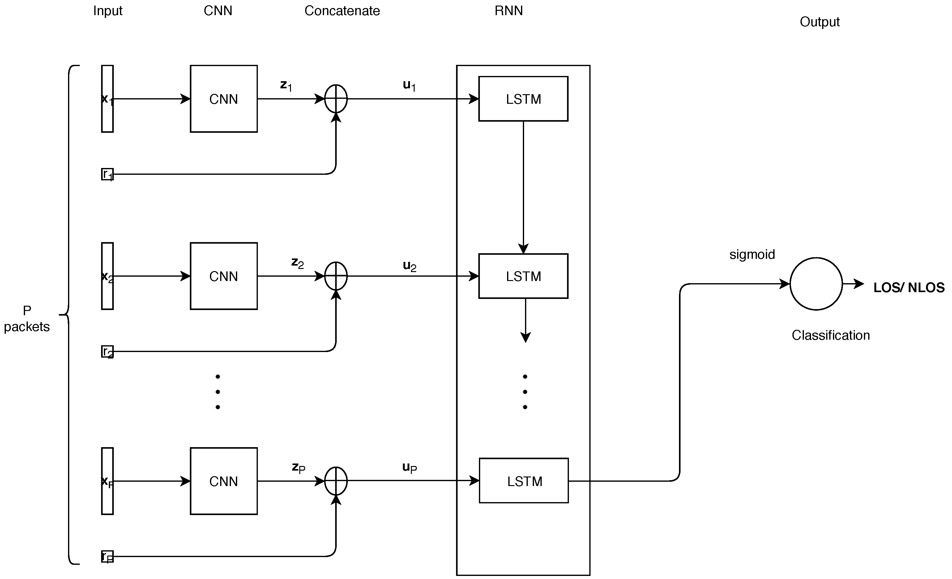
To classify LOS and NLOS in WLANs, we propose a novel CNNLSTM model. Figure 2 shows the overall framework of the proposed model, that comprise CNN and RNN segments. As shown in Figure 2, the CSIs form the input signals for the CNN, while the output of CNN concatenates with the RSSIs, and feed into the LSTMs for the LOS and NLOS classification.
4.1. CNN Part
Figure 3 shows the proposed CNN model, that comprises one input vector, L convolutional layers, and one output vector with size by a Flatten layer. The input vector for the pth packet transmission can be expressed as
where is the CSI for the packet transmission, and and are the real and imaginary parts of the complex value, respectively. The convolutional layer convolves the input regions locally using filter kernels, where each filter uses the same kernel to extract the local features of the input region. The output of a convolution operation at the layer for one filter is determined by
where is the kernel size of the filters, and are the weight and bias elements located at on the kernel, respectively, in the convolutional layer. In addition, represents a non-linearity activation function, that is typically given by the sigmoid, softsign, hyperbolic tangent (tanh) and rectified linear unit (reLU), etc. [31]. Without zero-padding, the output size is calculated as
where is a stride, which corresponds to how much a filter is shifted at a time. We put batch normalization (BN) after the non-linearity activation function applied after each CNN layer. The BN plays a role in regularization; its benefits are discussed in [32].
As shown in Figure 3, the CNN segment has L layers and we finally stress out the data to a vector with size by a Flatten layer. Note that CSI data is different from actual images so when applying the CNN, we need to change some structures from the normal CNN model. The first thing is to set the stride step by even numbers (2,4, etc.) in the first convolutional layer to guarantee the characteristic of complex input data. Because the size of the CSI packet is small, the second difference is that we do not apply any pooling layers, thereby significantly reducing the size of the input, leading to the loss of some important information to training in the RNN segment.
4.2. RNN Part
The RNN model is composed of LSTM modules and an output layer for classification. The input vector for the LSTM module is defined as where is an RSSI value for the packet transmission. The structure of the LSTM is shown in Figure 4. At the current time step p, the equations below describe the internal structure of the LSTM module:
where is the input to the LSTM block; , , , and are the input gate, the forget gate, the output gate, the cell state, and the output of the LSTM block, respectively. , , , and are the weights between the cell state and the input gate, the forget gate, the external output gate, and the output gate, respectively. , , ,and are the weights between the cell state and the input gate, the forget gate, the external output gate, and the output gate, respectively, and finally, , , , and are the additive biases of the input gate, the forget gate, the external output gate, and the output gate, respectively. The sigmoid function and the hyperbolic activation function are used as activation functions. In (7) and (8), the cell state, , and the output of the LSTM block, , are calculated using the outputs form the above gates in (6), where ⊙ denotes an element-wise multiplication.
Finally, for the NLOS and LOS condition decision, we put the feature vector extracted at the last LSTM cell through a single perceptron layer where P is the number of packet transmissions. The output of the model is calculated as follows:
where is the weight matrix that transfers the values in the Fully Connected (FC) layer to the output layer and b is a bias factor. In(9), the sigmoid function is used to transform the logit of the single neuron in the final stage to calculate the probability for classifying the LOS or NLOS.
We set for LOS conditions and for NLOS conditions. During the training stage, at each epoch, we select multiple batches from the set of input and output pairs to train and verify the proposed CNNLSTM model. Every parameter in the model is adjusted to minimize the following lost function
where N is the batch size of model, is the cost of the input and output pair that measures how accurately the model predicts the label that corresponds to the input. Among many choices of the loss function used in optimizing our model, we adopt the binary cross-entropy function, expressed by
where the superscript is used to indicate the index of the input and output pair.
To minimize the loss function, many variants of the gradient-descent method such as AdaGrad, AdaDelta, and Adam optimizers have been studied. These optimizers adaptively change the learning rate to properly minimize the loss function. In this study, we applied the Adam optimization algorithm to train our proposed CNNLSTM model as the Adam optimizer is straight-forward and saves memory and computational resources.
The process starts with random initialization of all the model parameters. During the training phase, the weight update takes place after a whole sequence has been propagated forward through the network. The error signals are calculated with respect to the Mean of Cross Entropy Losses cost function. The loss function was chosen as the natural cost function for the sigmoid output layer with the aim of maximizing the likelihood of classifying the input data correctly.
Once every parameter in the proposed CNNLSTM model is adjusted appropriately, the model can identify the channel condition based on the following simple hypothesis test
where and are null and alternative hypothesis, respectively, and denotes the decision threshold. We assume that, LOS detection rate is a true positive rate (TPR) corresponding to the portion of correct decisions among all measurements under the LOS condition. Similarly, NLOS detection rate is a true negative rate (TNR) corresponding to the portion of correct decisions over all measurements. These statistical values depend on the decisions.
5. Performance Evaluation
In this section, we will discuss the results of the proposed scheme using CSI and RSSI data with a total 100,000 packet transmissions. We assess several numbers of packet transmissions, , , and . We split our dataset into three parts: training, validation, and test sets. We use 70% of sample points to build our classification model during the training phase. 15% of data were used to compare the performances of the models in the validation phase. We selected the best model for the test phase. Finally, we applied our chosen model to the test set, the remaining 15% of the original data set, so as to evaluate how our model performs on unseen data. Note that, the test set was not used in the experiments.
The model was trained by truncated backpropagation through time [33] with Adam optimization [34] with an initial learning rate of 0.001. On the dataset, we used a minibatch [35] with a size of 128 for high efficiency. After each batch, the gradients were averaged and updated. We employed the early stopping method to stop the training when the validation accuracy becomes stagnant and does not increase after 10 epochs. We adopted the dropout method with a probability of 0.5 after the CNN layers and LSTM layer for regularization to avoid over-fitting problems [36].
In the CNN segment, we used hybrid hyper-parameters settings for the CNNs with high numbers, L of convolution layers to extract the implicit features of data. We applied the CNN models with a different number of filters, such as 16, 32, 64, 128, etc. with different kernel sizes, such as 2, 3, 4, etc., and with several kinds of popular activation functions, such as ReLU, tanh, sigmoid, etc. After testing out all the simulation settings, the best achieved model is as shown in Table 1. Here, we set number of CNN layers with kernel size, for the first layer, and for the second and third layer. In the first and second CNN layers, we use and filters with the softplus activation function. and are used for the third CNN layer.
In the RNN segment, we also set different the number of units in LSTM layer, , such as 5, 10, 20, etc., to obtain the best result for our model.
Figure 5 shows the convergence of the model over epochs for the training and validation set. It can be seen that, the accuracy of the training set shows a trend of improvement in performance after each epoch. Conversely, the accuracy of the validation set decrease and fluctuates after reaching the top point of 96.32%. To avoid wasting time in training the data, we used the early stopping method that automatically stops the model if the accuracy of the validation set does not improve after several epochs (in our model, this value was set to 10). The peak point of the highest accuracy for the validation set occurred in epoch 21 and was marked by X symbol in the figure.
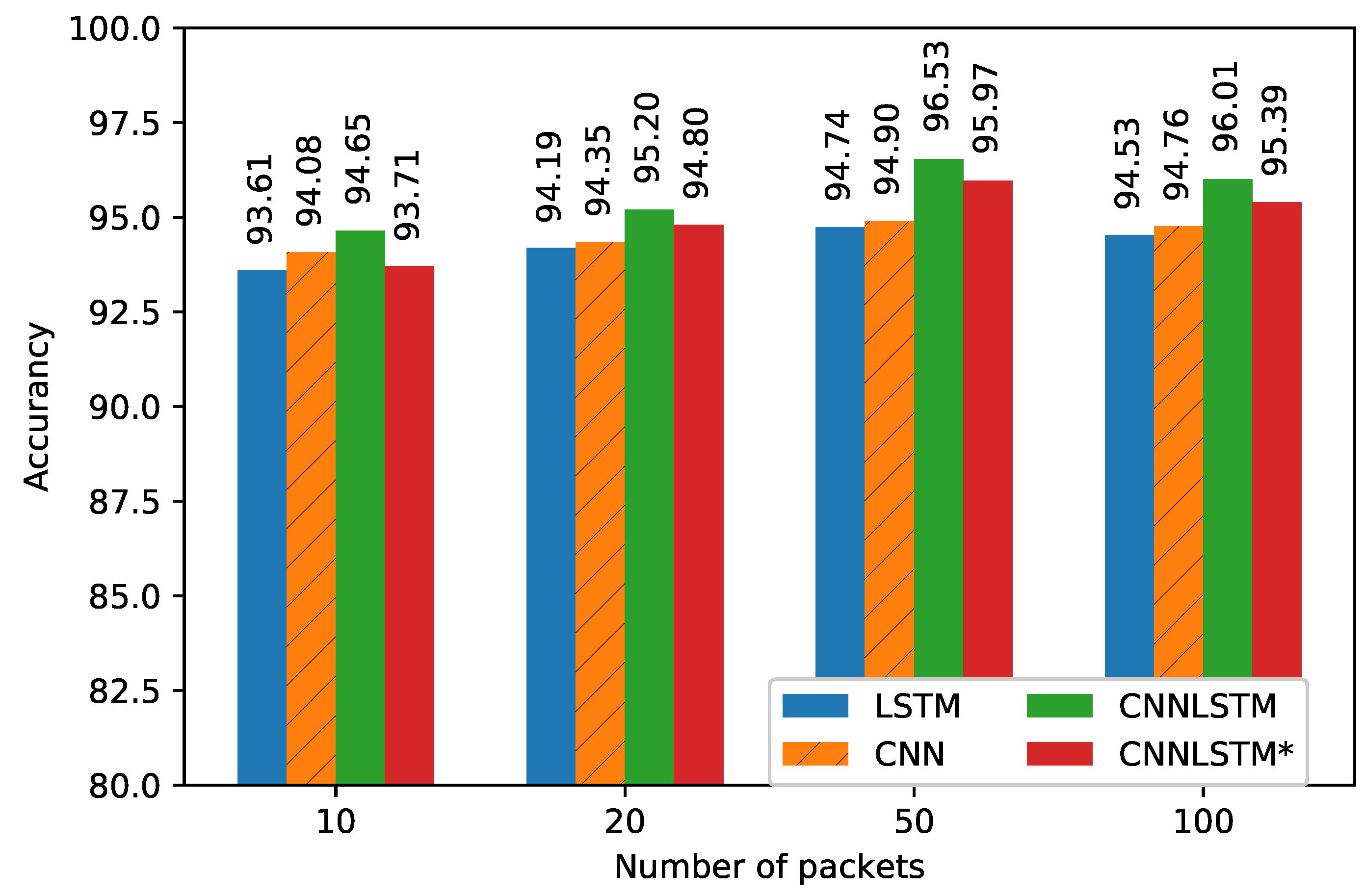
In this paper, we also implemented CNN methods and compared them with the conventional method LSTM method. The CNN model was also optimized similarly to the proposed CNN segment, except here, instead of the LSTM layer, we added the Flatten layer after the final CNN layer. The LSTM model only learns time relative sequence information whereas the CNN model focuses on extracting implicit features that contain space information, while our proposed model offers both of these advantages. Figure 6 illustrates the performance of the proposed model with various values of P for the test set. It can be seen that the best outcome was obtained at . Even if P is increased to 100, the performance shows a decreasing trend for all models. Hence, in the results shown below, we use to compare to the building data.
Table 2 summarizes the performances decision thresholds that are selected to maximize the average LOS/NLOS detection rate for the LSTM, CNN, and CNNLSTM models. As can be seen, the CNNLSTM model outperforms the other models in both accuracy and average detection rate for all values of P. Note that CNNLSTM* denotes a model that applies the absolute values of CSI data. It offers slightly better performance than the LSTM and CNN models while using simpler data, so we can consider it as a choice when generating data from practical instruments. The input signal for the CNN segment in this case can be written as
where is the amplitude value of the CSI for the packet transmission.
Table 3 shows the total training time and the number of parameters of the LSTM, CNN and proposed CNNLSTM models, where an NVIDIA Titan X GPU 1.4 GHz with 3584 cores is used for simulations. The total training time for the proposed CNNLSTM is comparable to the CNN and LSTM models because the proposed model takes only 21 epochs to converge to the optimal solution. The number of parameters for the proposed CNNLSTM is larger than the LSTM model. However, the memory requirement is less demanding in the test time evaluation because there is no backward propagation. In addition, the proposed CNNLSTM* reduces the total training time and number of parameters compared to the proposed CNNLSTM.
In Figure 7, we use the receiver operating characteristic (ROC) curve, that describes the relationship between TPR and FPN. If the performance is better, the ROC curve will approach a point in the upper left edge, that implies perfect discrimination. As we can see, the LSTM model has worse performance. Conversely, the proposed CNNLSTM model offers the best result because its area under curve (AUC) of 0.9928 approximates with perfect result of 1 [18,19,37].
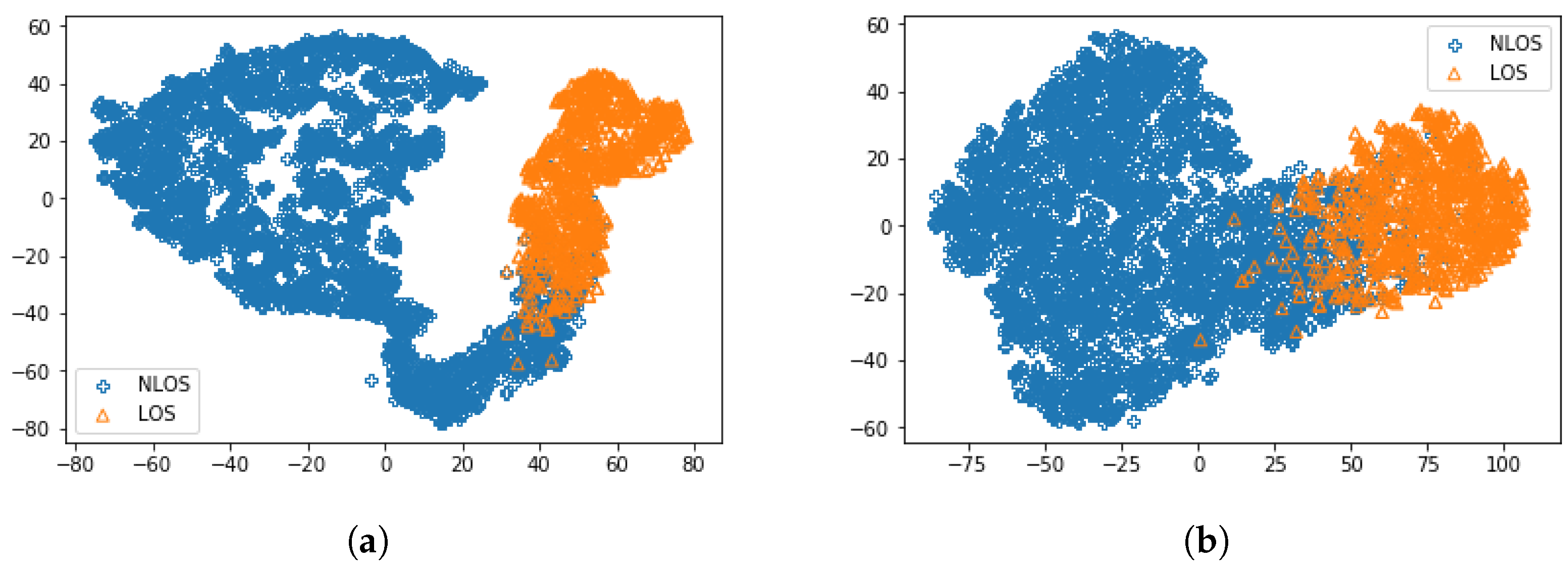
To further understand what is inside the model, we analyze the internal representations of the trained network. Following the training procedure, the hidden state vector of the last LSTM module was used to visualize the trained network. Figure 8 shows t-SNE representations using 5000 different inputs from the training set of the proposed method and conventional LSTM method [16], where t-SNE aims to project the high dimensional vectors to two-dimensional space while retaining their pairwise similarity [38]. In the figure, we can see that the hidden state for the proposed method was much more dispersed compared to the hidden state for the conventional method [16]. This explains the improved accuracy based on feature extraction by using CNN segment in the proposed CNNLSTM.
6. Conclusions
In this paper, we proposed a deep learning model to identify channel conditions by combining CNN and RNN. In the proposed CNNLSTM model, the CNN captured the feature from frequency-domain characteristics of CSIs and then LSTMs extracted the temporal feature from RSSI and the output of CNN. In addition, a CNNLSTM model with the absolute value of CSIs was proposed to reduce the complexity with slightly better performance than the conventional models. The proposed methods were verified under indoor environments for WLANs and achieved higher accuracy than the conventional LSTM model in classifying LOS and NLOS. In future work, we would like to investigate the performance of the proposed CNNLSTM models in outdoor environments to expand the range of applications of the algorithm.
Author Contributions
V.-H.N. and Y.-H.K. conceived the idea of the proposed scheme and performed the modeling and simulation of the proposed scheme. M.-T.N. and J.C. provided substantial comments on the performance analysis of the proposed scheme.
Funding
This research was supported in part by Korea Electric Power Corporation (Grant number:R18XA01) and in part by the Basic Science Research Program through the National Research Foundation of Korea (NRF) funded by the Ministry of Science and ICT (NRF-2017R1C1B1012259).
Conflicts of Interest
The authors declare no conflict of interest.
References
- McNeff, J.G. The global positioning system. IEEE Trans. Microw. Theory Tech. 2008, 50, 645–652. [Google Scholar] [CrossRef]
- Cui, K.; Chen, G.; Xu, Z.; Richard, D.R. Line-of-sight visible light communication system design and demonstration. In Proceedings of the 7th International Symposium on Communication Systems, Networks & Digital Signal Processing (CSNDSP 2010), Newcastle upon Tyne, UK, 21–23 July 2010; pp. 621–625. [Google Scholar]
- Dialani, J.C.; Patel, A.; Jindal, R.P. Performance measurements of IEEE 802.11 a wireless LANs in presence of ultrawideband interference. In Proceedings of the 2006 IEEE Sarnoff Symposium, Princeton, NJ, USA, 27–28 March 2006; pp. 1–4. [Google Scholar]
- Aiello, G.R.; Rogerson, G.D. Ultra-wideband wireless systems. IEEE Microw. Mag. 2003, 2, 36–47. [Google Scholar] [CrossRef]
- Kaemarungsi, K. Distribution of WLAN received signal strength indication for indoor location determination. In Proceedings of the 1st International Symposium on Wireless Pervasive Computing, Phuket, Thailand, 16–18 January 2006. [Google Scholar]
- Seshadri, V.; Zaruba, G.V.; Huber, M. A bayesian sampling approach to in-door localization of wireless devices using received signal strength indication. In Proceedings of the Third IEEE International Conference on Pervasive Computing and Communications, Kauai Island, HI, USA, 8–12 March 2005; pp. 75–84. [Google Scholar]
- Wang, X.; Wang, Z.; O’Dea, B. A TOA-based location algorithm reducing the errors due to non-line-of-sight (NLOS) propagation. IEEE Trans. Veh. Technol. 2003, 1, 112–116. [Google Scholar] [CrossRef]
- Guvenc, I.; Chong, C.-C. A survey on TOA based wireless localization and NLOS mitigation techniques. IEEE Commun. Surv. Tutor. 2009, 11, 107–124. [Google Scholar] [CrossRef]
- Chan, Y.-T.; Tsui, W.-Y.; So, H.-C.; Ching, P.-C. Time-of-arrival based localization under NLOS conditions. IEEE Trans. Veh. Technol. 2006, 1, 17–24. [Google Scholar] [CrossRef]
- Venkatraman, S.; Caffery, J.; You, H.-R. A novel TOA location algorithm using LOS range estimation for NLOS environments. IEEE Trans. Veh. Technol. 2004, 5, 1515–1524. [Google Scholar] [CrossRef]
- Caire, G.; Shamai, S. On the capacity of some channels with channel state information. IEEE Trans. Inf. Theory 1999, 6, 2007–2019. [Google Scholar] [CrossRef]
- Marzetta, T.L.; Hochwald, B.M. Fast transfer of channel state information in wireless systems. IEEE Trans. Sign. Process. 2006, 4, 1268–1278. [Google Scholar] [CrossRef]
- Zhou, Z.; Yang, Z.; Wu, C.; Sun, W.; Liu, Y. LiFi: Line-of-sight identification with WiFi. In Proceedings of the IEEE INFOCOM 2014–IEEE Conference on Computer Communications, Toronto, ON, Canada, 27 April–2 May 2014; pp. 2688–2696. [Google Scholar]
- Zhou, Z.; Yang, Z.; Wu, C.; Shangguan, L.; Cai, H.; Liu, Y.; Ni, L.M. WiFi-based indoor line-of-sight identification. IEEE Trans. Wirel. Commun. 2015, 11, 6125–6136. [Google Scholar] [CrossRef]
- Wu, C.; Yang, Z.; Zhou, Z.; Qian, K.; Liu, Y.; Liu, M. PhaseU: Real-time LOS identification with WiFi. IEEE Trans. Wirel. Commun. 2015, 14, 2038–2046. [Google Scholar]
- Choi, J.S.; Lee, W.H.; Lee, J.H.; Lee, J.H.; Kim, S.C. Deep Learning Based NLOS Identification with Commodity WLAN Devices. IEEE Trans. Veh. Technol. 2018, 4, 3295–3303. [Google Scholar] [CrossRef]
- Kim, K.S.; Lee, S.; Huang, K. A scalable deep neural network architecture for multi-building and multi-floor indoor localization based on Wi-Fi fingerprinting. Big Data Anal. 2018, 3, 4. [Google Scholar] [CrossRef] [Green Version]
- Abbas, R.; Hussain, A.J.; Al-Jumeily, D.; Baker, T.; Khattak, A. Classification of Foetal Distress and Hypoxia Using Machine Learning Approaches. Int. Conf. Intell. Comput. 2018, 767–776. [Google Scholar]
- Amin, A.; Shah, B.; Khattak, A.M.; Baker, T.; Anwar, S. Just-in-time Customer Churn Prediction: With and Without Data Transformation. In Proceedings of the IEEE Congress on Evolutionary Computation (CEC), Rio de Janeiro, Brazil, 8–13 July 2018; pp. 1–6. [Google Scholar]
- Alshabandar, R.; Hussain, A.; Keight, R.; Laws, A.; Baker, T. The Application of Gaussian Mixture Models for the Identification of At-Risk Learners in Massive Open Online Courses. In Proceedings of the 2018 IEEE Congress on Evolutionary Computation (CEC), Rio de Janeiro, Brazil, 8–13 July 2018; pp. 1–8. [Google Scholar]
- Cireşan, D.C.; Meier, U.; Gambardella, L.M.; Schmidhuber, J. Deep, big, simple neural nets for handwritten digit recognition. Neural Comput. 2010, 22, 3207–3220. [Google Scholar] [CrossRef] [PubMed]
- Sharif Razavian, A.; Azizpour, H.; Sullivan, J.; Carlsson, S. CNN features off-the-shelf: An astounding baseline for recognition. In Proceedings of the IEEE conference on computer vision and pattern recognition workshops, Columbus, OH, USA, 24–27 June 2014; pp. 806–813. [Google Scholar]
- Yin, W.; Kann, K.; Yu, M.; Schütze, H. Comparative study of cnn and rnn for natural language processing. arXiv, 2017; arXiv:1702.01923. Available online: https://arxiv.org/abs/1702.01923(accessed on 7 February 2017).
- Chen, H.; Zhang, Y.; Li, W.; Tao, X.; Zhang, P. ConFi: Convolutional neural networks based indoor wi-fi localization using channel state information. IEEE Access 2017, 5, 18066–18074. [Google Scholar] [CrossRef]
- Graves, A.; Mohamed, A.R.; Hinton, G. Speech recognition with deep recurrent neural networks. In Proceedings of the Acoustics, speech and signal processing (icassp), 2013 ieee international conference, Vancouver, BC, Canada, 26–31 May 2013; pp. 6645–6649. [Google Scholar]
- Pascanu, R.; Gulcehre, C.; Cho, K.; Bengio, Y. How to construct deep recurrent neural networks. arXiv, 2013; arXiv:1312.6026. Available online: https://arxiv.org/abs/1312.6026(accessed on 24 April 2014).
- Hochreiter, S. The vanishing gradient problem during learning recurrent neural nets and problem solutions. Int. J. Uncertain. Fuzziness Knowl. Based Syst. 1998, 6, 107–116. [Google Scholar] [CrossRef]
- Tsironi, E.; Barros, P.; Weber, C.; Wermter, S. An analysis of convolutional long short-term memory recurrent neural networks for gesture recognition. Neurocomputing 2017, 268, 76–86. [Google Scholar] [CrossRef]
- Tzirakis, P.; Trigeorgis, G.; Nicolaou, M.A.; Schuller, B.W.; Zafeiriou, S. End-to-end multimodal emotion recognition using deep neural networks. IEEE J. Sel. Top. Sign. Process. 2017, 11, 1301–1309. [Google Scholar] [CrossRef]
- Sainath, T.N.; Vinyals, O.; Senior, A.; Sak, H. Convolutional, long short-term memory, fully connected deep neural networks. In Proceedings of the 2015 IEEE International Conference on Acoustics, Speech and Signal Processing (ICASSP), Brisbane, Australia, 19–24 April 2015; pp. 4580–4584. [Google Scholar]
- Mishkin, D.; Sergievskiy, N.; Matas, J. Systematic evaluation of CNN advances in the ImageNet. Comput. Vis. Image Underst. 2017, 161, 11–19. [Google Scholar] [CrossRef]
- Sergey Ioffe and Christian Szegedy, Batch Normalization: Accelerating Deep Network Training by Reducing Internal Covariate Shift. arXiv, 2015; arXiv:1502.03167. Available online: https://arxiv.org/abs/1502.03167(accessed on 2 March 2015).
- Werbos, P.J. Backpropagation through time: What it does and how to do it. Proc. IEEE 1990, 78, 1550–1560. [Google Scholar] [CrossRef]
- Kingma, D.P.; Ba, J. Adam: A Method for Stochastic Optimization. arXiv, 2014; arXiv:1412.6980. Available online: https://arxiv.org/abs/1412.6980(accessed on 30 January 2017).
- Cotter, A.; Shamir, O.; Srebro, N.; Sridharan, K. Better mini-batch algorithms via accelerated gradient methods. Adv. Neural Inf. Process. Syst. 2011, 1647–1655. [Google Scholar]
- Srivastava, N.; Hinton, G.; Krizhevsky, A.; Sutskever, I.; Salakhutdinov, R. Dropout: A Simple Way to Prevent Neural Networks from Overfitting. J. Mach. Learn. Res. 2014, 15, 1929–1958. [Google Scholar]
- Hanley, J.A.; McNeil, B.J. The meaning and use of the area under a Receiver Operating Characteristic (ROC) Curve. Radiology 1982, 143, 29–36. [Google Scholar] [CrossRef] [PubMed]
- Maaten, L.V.D.; Hinton, G. Visualizing Data using t-SNE. J. Mach. Learn. Res. 2008, 9, 2579–2605. [Google Scholar]
Figure 1.
The experiment setup.

Figure 2.
The overall framework of the proposed CNNLSTM.

Figure 3.
Proposed one-dimensional CNN model.

Figure 4.
The structure of the LSTM.

Figure 5.
Performance convergence versus epochs.

Figure 6.
Performances of the models depend on the number of packets.

Figure 7.
ROC curves of LOS identification using the proposed CNNLSTM and other methods.

Figure 8.
tSNE representation of 5000 training samples for (a) proposed CNNLSTM and (b) conventional LSTM.
Figure 8.
tSNE representation of 5000 training samples for (a) proposed CNNLSTM and (b) conventional LSTM.


Table 1.
Details of proposed CNNLSTM model.
| Layer Type | Activation | Kernel Size | Stride | Filter | Output Shape |
|---|---|---|---|---|---|
| Input | 50 × 112 × 1 | ||||
| Convolution | softplus | 8 | 2 | 32 | 50 × 53 × 32 |
| Convolution | softplus | 2 | 1 | 16 | 50 × 52 × 16 |
| Convolution | reLU | 2 | 1 | 8 | 50 × 51 × 8 |
| Flatten | _ | _ | _ | _ | 50 × 408 |
| Concatenate with RSSI | _ | _ | _ | _ | 50 × 409 |
| LSTM | _ | _ | _ | 10 | 10 |
| FC | sigmoid | _ | _ | 1 | 1 |
Table 2.
Performances according to the models.
| Model | Decision Threshold | Avg Detection Rate | Accuracy |
|---|---|---|---|
| LSTM | 0.332970 | 0.94920 | 94.57 |
| CNN | 0.372340 | 0.94310 | 94.90 |
| CNNLSTM | 0.302848 | 0.95989 | 96.53 |
| CNNLSTM* | 0.225334 | 0.95141 | 95.97 |
Table 3.
The training time and number of parameters of the models.
| Model | Time (s) | Epochs | Total Training Time (s) | Number of Parameters |
|---|---|---|---|---|
| LSTM | 9 | 37 | 333 | 5011 |
| CNN | 16 | 25 | 400 | 22,463 |
| CNNLSTM | 17.5 | 21 | 367.5 | 18,863 |
| CNNLSTM* | 15 | 23 | 345 | 9679 |
© 2018 by the authors. Licensee MDPI, Basel, Switzerland. This article is an open access article distributed under the terms and conditions of the Creative Commons Attribution (CC BY) license (http://creativecommons.org/licenses/by/4.0/).
Share and Cite
MDPI and ACS Style
Nguyen, V.-H.; Nguyen, M.-T.; Choi, J.; Kim, Y.-H. NLOS Identification in WLANs Using Deep LSTM with CNN Features. Sensors 2018, 18, 4057. https://doi.org/10.3390/s18114057
AMA Style
Nguyen V-H, Nguyen M-T, Choi J, Kim Y-H. NLOS Identification in WLANs Using Deep LSTM with CNN Features. Sensors. 2018; 18(11):4057. https://doi.org/10.3390/s18114057
Chicago/Turabian StyleNguyen, Viet-Hung, Minh-Tuan Nguyen, Jeongsik Choi, and Yong-Hwa Kim. 2018. "NLOS Identification in WLANs Using Deep LSTM with CNN Features" Sensors 18, no. 11: 4057. https://doi.org/10.3390/s18114057
Note that from the first issue of 2016, this journal uses article numbers instead of page numbers. See further details here.