Article

Evaluation of Prestress Loss Distribution during Pre-Tensioning and Post-Tensioning Using Long-Gauge Fiber Bragg Grating Sensors

1
Department of Civil Engineering, Fuzhou University, Fuzhou 350108, China
2
Hebei Province Key Laboratory of Evolution and Control of Mechanical Behavior in Traffic Engineering Structure, Shijiazhuang Tiedao University, Shijiazhuang 050043, China
3
CSCEC Strait Construction and Development Co., LTD, Fuzhou 350015, China
4
Fujian Provincial Key Laboratory of Advanced Technology and Informatization in Civil Engineering, Fujian University of Technology, Fuzhou 350118, China
*
Author to whom correspondence should be addressed.
Sensors 2018, 18(12), 4106; https://doi.org/10.3390/s18124106
Submission received: 30 October 2018 / Revised: 17 November 2018 / Accepted: 18 November 2018 / Published: 23 November 2018
(This article belongs to the Special Issue Smart Sensors and Smart Structures)

Abstract

:
Prestress loss evaluation in prestressed strands is essential for prestressed structures. However, the sensors installed outside the duct can only measure the total prestress loss. The sensors attached on strands inside the duct also have several problems, such as inadequate durability in an aggressive environment and vulnerability to damage during tensioning. This paper proposes a new installation method for long-gauge fiber Bragg grating (LFBG) sensors to prevent accidental damage. Then the itemized prestress losses were determined in each stage of the pre-tensioning and post-tensioning according to the LFBG measurements. We verified the applicability of the LFBG sensors for prestress monitoring and the accuracy of the proposed prestress loss calculation method during pre-tensioning and post-tensioning. In the pre-tensioning case, the calculated prestress losses had less deviation from the true losses than those obtained from foil-strain gauges, and the durability of the LFBG sensors was better than foil-strain gauges, whereas in post-tensioning case, the calculated prestress losses were close to those derived from theoretical predictions. Finally, we monitored prestress variation in the strand for 90 days. The itemized prestress losses at each stages of post-tensioning were obtained by the proposed calculation method to show the prospect of the LFBG sensors in practical evaluation.

1. Introduction

Prestressing of steel strands provides reversal stress to counteract in-service stress partially or entirely, improve the crack resistance, and reduce the deflection of prestressed structures. Thus, the tensile stress in steel strands can be maintained over time. However, the applied prestress may decrease gradually due to various reasons, such as the stress relaxation in the steel strands, concrete creep and shrinkage, friction between the strand and duct, and deformation of anchoring devices [1]. Moreover, long-term factors including aggressive environment, pitting, stress corrosion, and hydrogen embrittlement can decrease prestressing further and trigger a fracture of the strand that gives rise to accidents, causing the degradation of the nuclear containment vessel [2], the decrease in seismic performance of the concrete frame [3], and the collapse of a bridge [4]. Therefore, measuring and evaluating prestress loss of steel strand is imperative for maintenance and accurate assessment of prestressed structures.
Current sensing techniques for prestress loss measurement can be grouped into two categories: global measurements and local measurements. The global measurements are performed via elastomagnetic sensors [5,6,7], stress waves [8,9], Anchorage-Measurement-Access system [10,11], frequency [12,13], and modal parameters [14]. A common characteristic of the global measurement techniques is that the sensors are usually placed outside anchoring devices to obtain a “global” prestress of the strand. However, this approach has critical drawbacks. First, the “global” value fails to reflect the itemized prestress losses distributing along the strand. Moreover, most global measurements are indirect, complicated in data processing, and disturbed easily by electromagnetic interference. Last, the global measurement does not provide enough sensitivity to detect stress variations that may be quite small compared to the total stress of a prestressed strand due to micro cracks.
To overcome these disadvantages, researchers have focused on the local measurement that place the sensor on the surface of the strand to directly monitor prestresses at some pre-designated points. The local measurement is applied based on some electric sensors, such as strain gauges [15,16], piezoelectric transducer actuator [17] and so on. However, local measurement is more challenging to perform than global measurement due to the following three reasons. First, if the duct has a curved profile between the ends, the sensor or connecting line may be dislocated and damaged by the friction between the strand and duct during tensioning. Second, the interspace is small between the strand and duct. Some sensors, such as the elastomagnetic sensors, cannot be installed into the duct due to their size. The third reason is that grout used to fill the duct after tensioning may trigger a short circuit to the electric sensor without resin isolation.
The above challenges could be overcome using a fiber Bragg grating (FBG) sensor that is more suitable for long-term prestress monitoring than an electric sensor due to its small size, light weight, high stability, and durability. In recent years, FBG sensors have been widely used for dynamic strain-stress and vibration measurements in bridges [18,19,20], scour monitoring [21,22], reinforcement corrosion [23,24], and leakages in concrete structures and pipelines [25,26,27,28]. Two kinds of FBG sensors have been proposed for prestress monitoring. The first type is named as “smart strand” consisting of six helical wires and a core wire embedded an FBG sensor [29,30,31,32,33]. Although the FBG sensor can accurately measure prestress in the core wire, the “smart strand” also has two drawbacks in practice. First, for cost reduction, the position of each FBG sensor in a “smart strand” is predetermined in the production stage, and the distance between adjacent sensors is usually identical. However, these predetermined positions and distances may not match the required positions and distances in practical construction. Second, because the core wire is surrounded closely by six helical wires, it is difficult to connect the embedded FBG sensor in the core wire to the optical cable used to transmit the optical signal.
An improved “smart strand” type sensor has been proposed for monitoring prestress distribution by combining the Brillouin optical time domain analysis/refectory (BOTDA/R) sensor and the FBG sensor along a single optical fiber to solve this problem [34,35]. However, the measurement error of the BOTDA/R sensor was at least dozens of micro-strain, reducing the accuracy of the monitoring data. The results of Zhang’s experiments showed that the strain measurement error of AQ8603 (produced by Ando Electric Co. Ltd., Tokyo, Japan) based on the BOTDR technique was ±130 με (1.96 σ,σ = ±65 με) [36], which is larger than the AQ8603’s nominal precision of ±50 με. The measurement error of the NBX-6000 (produced by Neubrex Co. Ltd., Kobe, Japan) based on pulse-prepump Brillouin Optical Time Domain Analysis (PPP-BOTDA) was about ±80 με (2σ, σ = ±40 με), which is larger than the NBX-6000’s nominal precision of ±25 με [37]. The second type of FBG sensor comprises a grating packaged with a metal capillary [38,39]. Then the capillary-encapsulated FBG sensors are bonded on the surface of the strand by epoxy resin to measure the elongation. The shortcomings of this type of FBG sensors also exist. First, the elastic modulus of steel is far greater than that of resin, and the mechanical strength of most epoxy resins is limited. Thus, mechanical creep may occur in epoxy, when the epoxy is stressed to beyond 50% of its tensile strength [40], and the bonding may fail if the transmitting stress reaches 80% of the ultimate tensile strength of resin [41]. Second, the sensor is proposed to install in the space between two adjacent steel wires [39]. This installation method may lead to accidental damage to the sensor caused by the dislocation of adjacent wires during strand tensioning. Finally, because the strain distributed in each wire is not identical, the measurements from the sensor for a single wire may have a remarkable difference from the true strain of the strand.
We propose that the long-gauge fiber Bragg grating (LFBG) sensor [42] could overcome the abovementioned limitations. The LFBG sensor has a sensing gauge ranging from 0.1 to 1 m suggesting that the measured strain can represent the average elongation of all wires in the gauge length. Meanwhile, the LFBG sensor is packaged by epoxy-soaked fiber reinforced polymer (FRP) material because the elastic modulus of the epoxy-soaked FRP material is less than that of steel so that the bonding can safely transmit the strain from the strand to the sensor. Moreover, the durability of the LFBG sensor has been verified by the fatigue experiment and long-term durability tests in acidic, alkaline, and salt environments [43]. The applicability of the LFBG sensor was also confirmed in practical monitoring for measuring dynamic strain [44] and dynamic displacement [45], and observing the change in the neutral axis position [46]. However, little is known on the monitoring and calculation of prestress losses based on the LFBG sensor.
This paper is organized as follows: Section 2 introduces the structure and design of an LFBG sensor for prestress monitoring in a strand and proposes the installation procedure in practical operation. Based on the strain measurements from the installed LFBG sensors, Section 3 proposes a method to calculate the itemized prestress losses in both pre-tensioning and post-tensioning. Section 4 and Section 5 demonstrate the application of the proposed method experimentally and via in-site monitoring, respectively.

2. The Design and Installation of LFBG Sensors

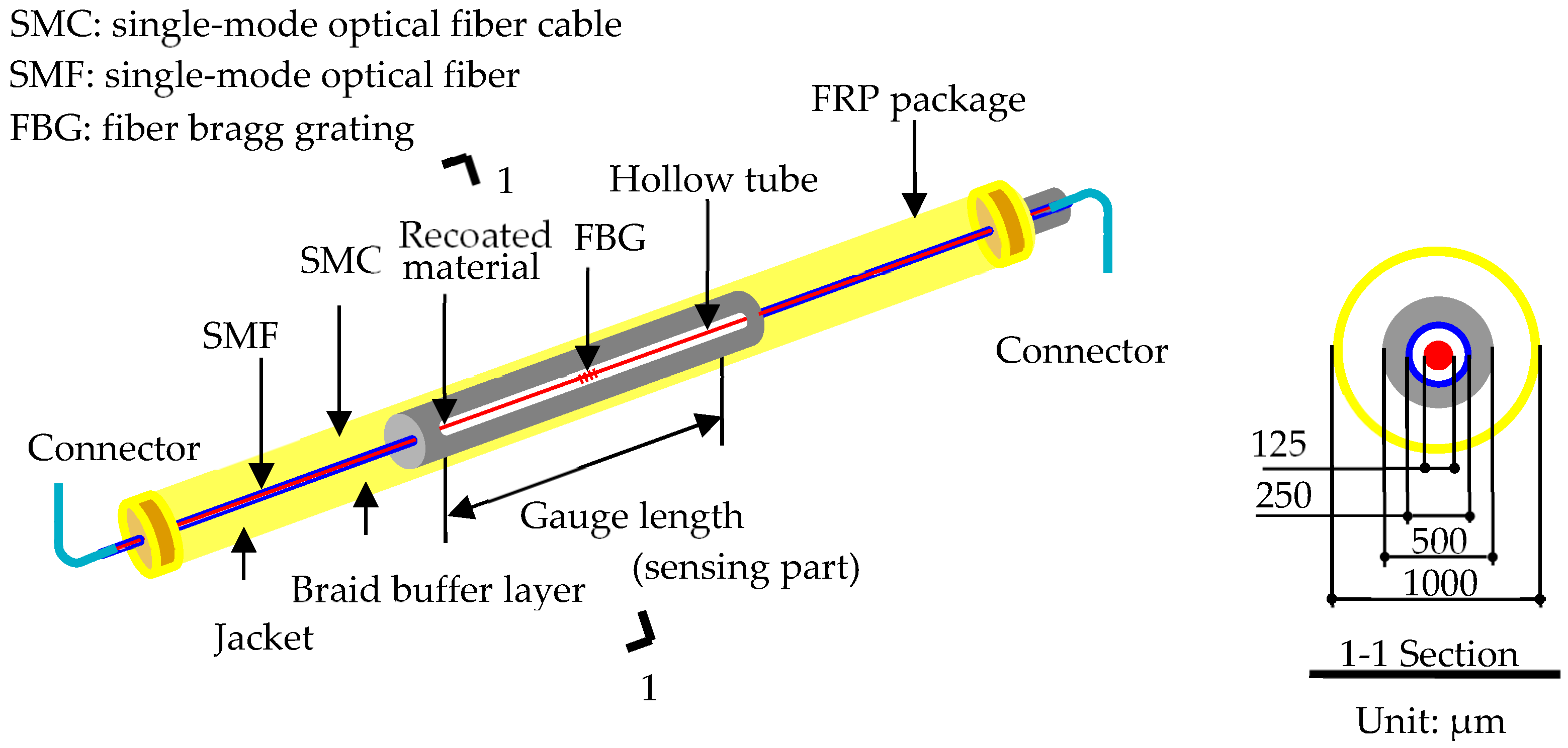
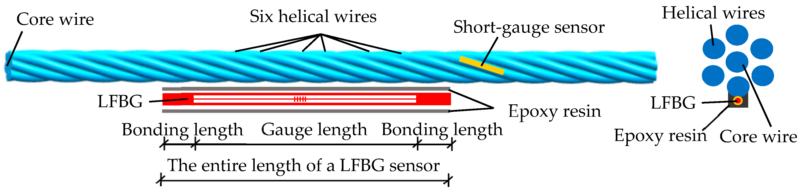
2.1. Introduction of the LFBG Strain Sensor

The structure of an LFBG sensor proposed by Li [42] is illustrated in Figure 1. A notable feature of this sensor is the use of an embedded and hollow polytetrafluoroethylene tube, inside which an FBG is sleeved and fixed at both ends, and the gauge length of the sensing part can be predetermined.
Moreover, the specific design is advantageous for numerous reasons: (i) The hollow tube used to encapsulate the FBG inside can ensure the strain at each point of the fiber optic is identical, and the measurement from the FBG equals the average strain over the gauge length directly. (ii) A special epoxy resin used to recoat the FBG can effectively prevent the slippage between the bare fiber optic and the epoxy resin. Meanwhile, the strain compatibility can be achieved between the FBG and epoxy resin until the measurement attains the breaking strain. This point is important for high stress-strain measurement in practical prestress monitoring. (iii) The bonding capability of the FRP material with structural materials, such as steel and concrete, is excellent. The FRP also has an excellent long-term durability and stability to prevent degradation due to corrosion and extreme environments.

2.2. Length Design of LFBG Sensor Installed on the Strand

As shown in Figure 2, the strand is composed of a linear core wire and six helical wires. Because the gauge lengths are no longer than several centimeters, most traditional strain sensors, such as the electric resistance strain gauge and the short-gauge FBG sensor, can obtain only the strain of one wire in the strand. However, this measurement cannot represent the true elongation of the strand. Therefore, the sensing part of the LFBG sensor needs to have a length that can touch all the six helical wires in a spiral. For example, the gauge length of an LFBG sensor is about 20–25 cm for stress monitoring to a 7-wire strand. Thus, the entire length of the LFBG sensor can reach 30–35 cm considering that bonding length of each end is set to about 5 cm. Generally, the total thickness of the sensor and the surrounding epoxy resin is less than 3 mm; this thickness is remarkably less than the diameter of a wire and space between the strand and duct.

2.3. Installation Procedure of the LFBG Sensor

The installation procedure is designed to prevent the installed LFBG sensors from accidental failure caused by friction between adjacent strands and between the strand and duct. The restraining block is used to separate adjacent strands and provide space to the sensor. Figure 3a,b show the designed restraining blocks for a 7-strand tendon and 3-strand tendon, respectively. Every block is assembled of two symmetrical parts by connecting bolts. The central hole of the block can contain the core strand and six helical strands that are separated by six grooves. The practical sketch of the restraining blocks on a 7-strand tendon is illustrated in Figure 3c. The distance over 50–60 cm between the two restraining blocks is long enough to contain the LFBG sensors installed on the strands.
As shown in Figure 4a–f, the installation procedure is outlined as follows:
(1)
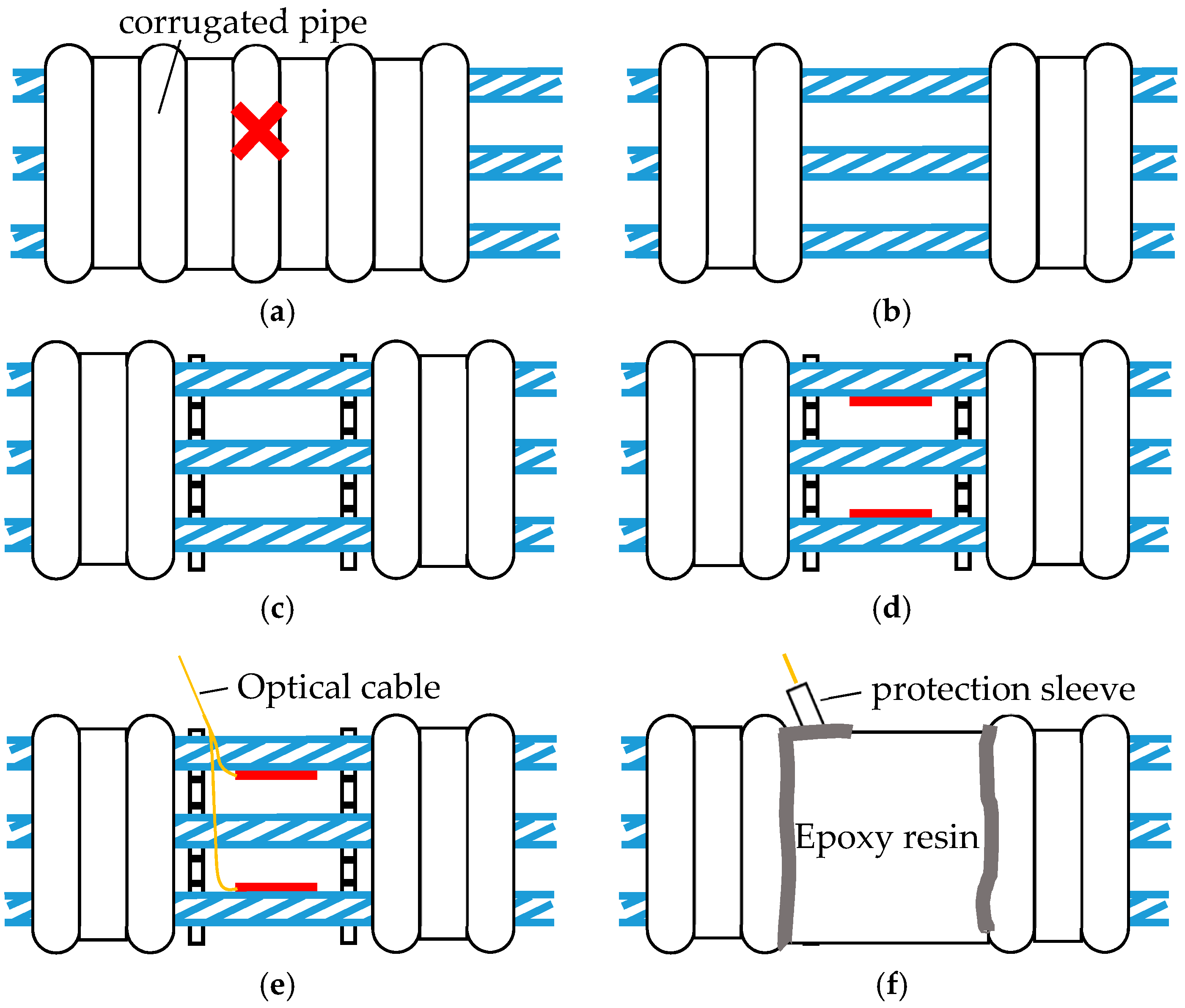
Mark the corresponding region on the corrugated pipe. Then let the strands pass through the marked corrugated pipe.
(2)
Peel the marked region of the corrugated pipe to expose the inner tendon. Clean the surface of the exposed tendons.
(3)
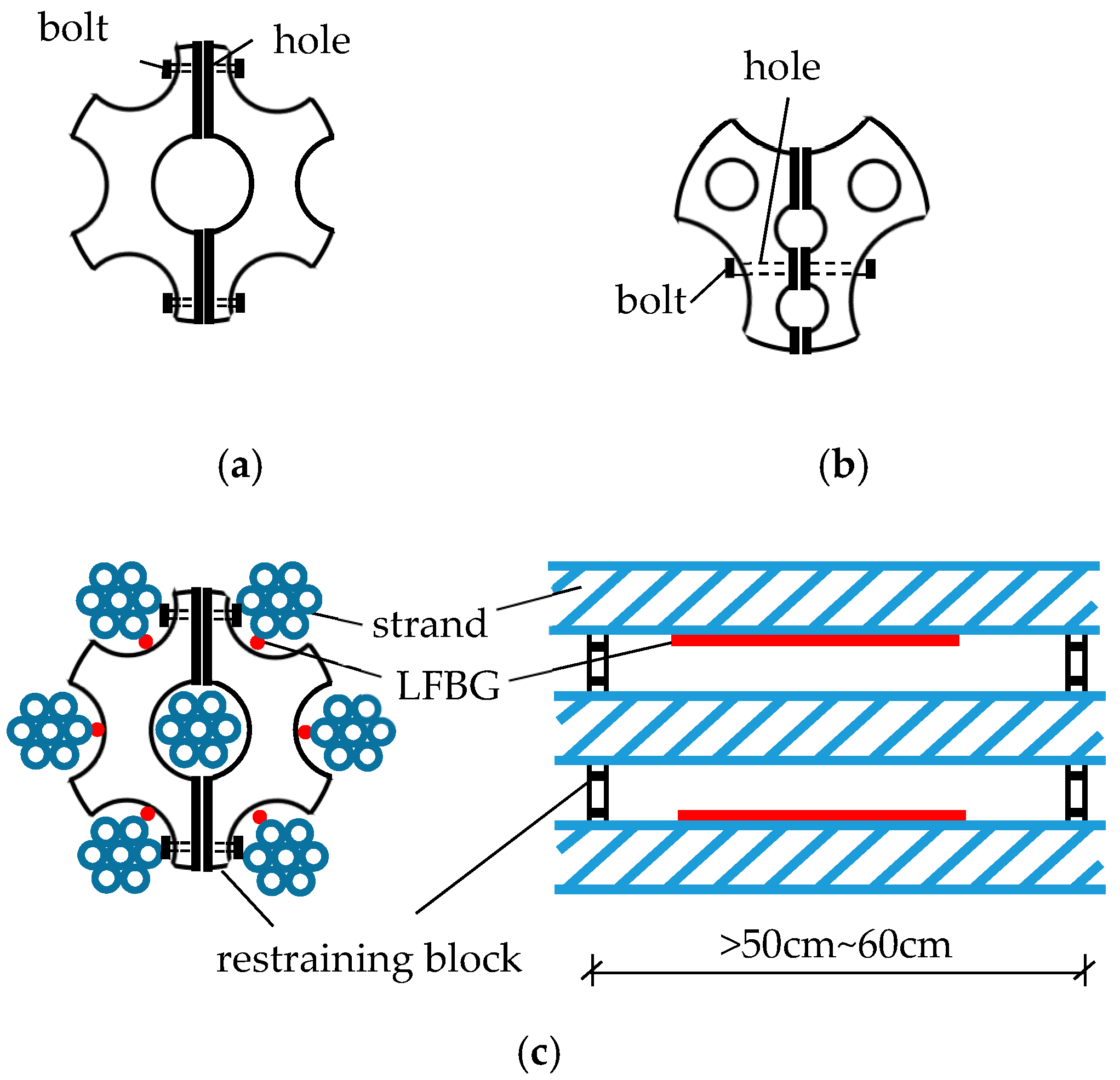
Install the restraining blocks and tighten the bolts.
(4)
Attach the LFBG sensors on the surface of the strands. The attachment position of the sensor on each outer strand should be pointed at and close to the core strand.
(5)
Let the optical cable pass through a protective sleeve and connect to the sensors.
(6)
Connect the protective sleeve to the corrugated pipe and use epoxy resin to seal off the contact area. Then the protection sleeve inside which the optical cable is placed can be extended away from the corrugated pipe to the nearest vent hole or drain hole.

3. The Calculation Method for Itemized Prestress Losses Based on the LFBG Measurements

The discussion proposes an optimized sensor configuration for pre-tensioning and post-tensioning and gives the calculation method for itemized prestress losses in both pre-tensioning and post-tensioning based on the LFBG measurements.

3.1. The Itemized Prestress Losses

In the Chinese Code [47], the total prestress loss comprises seven itemized prestress losses named as σl1σl7. σl1 is the anchorage-seating loss. σl2 is the frictional loss containing the loss due to the friction between tendons and duct (σl2,I) and the loss due to draw-in of the wedge (σl2,II). σl3 is the loss due to the temperature difference between the tendon and the abutments in concrete curing. σl4 is the loss due to steel relaxation. σl5 is the loss due to creep and shrinkage of concrete. σl6 is the loss due to the case in which spiral prestressed rebar in annular structure, such as nuclear containment vessel, is extruded by adjacent concrete. σl7 is the loss due to elastic shortening of concrete.
These seven itemized prestress losses are broadly classified into two groups: (1) immediate reductions during prestressing of the tendons and the prestress transferring from the tendons to the concrete members; and (2) time-dependent reductions occurring gradually during the in-service life of the structures. The immediate reductions contain σl1, σl2, σl3, σl6, and σl7. σl4, and σl5 belong to the time-dependent reductions.

3.2. The Case of Pre-Tensioning

As shown in Figure 5a–c, two abutments are fixed securely at both ends of a prestressing bed, and a high-strength steel tendon is pulled between the abutments before the concrete casting. When the concrete attains the required strength for prestressing, the tendon is cut from the abutments, and the prestress is transferred from the tendon to the concrete member through the bond between them. According to the Chinese Code [47], the total loss σ is the sum of several itemized prestress losses shown in Equation (1):
σ = σ l 1 + σ l 2 + σ l 3 + σ l 4 + σ l 5 + σ l 7  
and the term σl2,I does not exist in pre-tensioning.
A pre-tensioning beam is a typical kind of simply-supported beam. As illustrated in Figure 5, the LFBG sensors can be set on these regions of the tendon as follows: (1) regions near the ends of the beam (R1 and R3); (2) region near the mid-span of the beam (R2). The reason for the former choice is that σl1 and σl2,II constitute the main part of immediate losses, and σl3 and σl4 can be considered to be uniformly distributed along the tendon. The reason for the latter is that the mid-span usually has the maximum moment under the action of daily loads.
Five stages (Stages a–e) exist in a prestressed structure from pre-tensioning to load bearing. Of those, Stages a–d are shown in Figure 5a–c, and Stage e represents the in-service stage of the structure. The measured strains at R1–R3 at Stages a–d are set as ε a R i ~ ε d R i (i = 1–3), respectively. The superscript Ri denotes the variable located at Ri (i = 1–3). The subscript a-d implies that the variable is used at Stages a-d, respectively.
At the tensioning stage (Stage a), the relationship between the tensioning force and monitored strain is:
F = A t E t ε a R i   ( i =   1 3 )
where At and Et are the area and elastic modulus of prestressing tendon, respectively. F is the tensioning force obtained by the load cell. The value of Et is determined by a tensile test carried out in the laboratory. No prestress loss occurs at this stage.
σl1 and σl2 occur at Stage b of transferring the tensioning force from jack to prestressing bed. However, it is difficult to divide them without using special measurements, so the sum of σl1 and σl2 is shown as follows:
σ l 1 + σ l 2 = σ l 1 + σ l 2 , II E t ( ε a R 1 ε b R 1 )  
At Stage c of concrete member curing, σl3 and σ l 4 R i begin to appear. Because the low-relaxation prestressing strand can finish its relaxation in several hundreds of hours, σ l 4 R i can be obtained entirely in Stage c. Thus, σl3 and σ l 4 R i can be respectively calculated by Equations (4) and (5):
σ l 3 = E t α t Δ t  
σ l 4 R i = E t ( ε b R i ε c R i α t Δ t )   ( i =   1 ~ 3 )
At Stage d, the tendons between the beam and the abutment are cut off, and the prestress is resisted by the entire section of the beam. At this time, σ l 7 R i , which can be obtained by Equation (6) comes into play:
σ l 7 R i = E t ( ε c R i ε d R i )   ( i   =   1 ~ 3 )
At the in-service stage (Stage e), σ l 5 R i can be obtained by Equation (7) when the live load is not applied on the structure:
σ l 5 R i = E t ( ε d R i ε e R i )   ( i   =   1 ~ 3 )
Finally, substituting Equations (3)–(7) into Equation (1), the total prestress losses at different locations of the structure are obtained.

3.3. The Case of Post-Tensioning

A remarkable limitation of the pre-tensioning system is that the tendons always have to be straight. However, the post-tensioning system enables the tendons to keep a curved profile before and after tensioning. The ducts inside which the tendons are placed can be fixed to the reinforcements to remain in the desired profile. Then, once the concrete reaches the desired strength, the tendons are tensioned and anchored using external anchors rather than depending on the bond between tendon and concrete as in the pre-tensioning case. Figure 6a–b show the two stages of the post-tensioning procedure.
According to the Chinese Code [47], the total loss σ is the sum of several itemized prestress losses shown in Equation (8):
σ = σ l 1 + σ l 2 + σ l 4 + σ l 5 + σ l 6 + σ l 7  
As shown in Figure 6, σl6 is zero. σl2,I exists and does not equal to zero because the profile of the duct is usually curved. σl7 is zero unless the tendons are tensioned batch-wise.
The LFBG sensors can be set on the three regions (R1–R3) shown in Figure 6. In post-tensioning, the curve of the duct profile can be described as a combination of three parabolas. The two linking points between the three parabolas are key points in the design of prestressed structures. Thus, R1 and R3 are set to be near to these two linking points. R2 is set at the mid-span of the beam.
There are three stages (Stages a~c) in a post-tensioned structure from post-tensioning to load bearing. Stages a and b are the tensioning stage and the stage of anchoring, respectively. Stage c is the stage of grout curing and in-service stage of the structure that is shown in Figure 6b.
At Stage a, there are only the frictional losses σl2. In Equation (9), σ l 2 R i is the frictional loss in Ri:
σ l 2 R i = F / A t E t ε a R i   ( i =   1 ~ 3 )
At Stage b, the stress variation equals σ l 1 R i as follows:
σ l 1 R i = E t ( ε a R i ε b R i )  
At Stage c, the sum of σ l 4 R i and σ l 5 R i is shown in Equation (11). It also needs to be measured without live load action:
σ l 4 R i + σ l 5 R i = E t ( ε b R i ε c R i )  
This proposed method is also suitable for prestress loss calculation of more than one tendon in pre-tensioning and post-tensioning. Moreover, it is necessary to keep a distance between the sensor-placed regions near both ends of the strand and the anchor, since the violent variation of stress may threaten the safety of the LFBG sensors in prestress releasing. Finally, all the strain measurements should be updated by temperature compensation.

4. Verification for The Prestress Loss Monitoring Using LFBG Sensor: Experiment

This experiment in this study has two main purposes: to verify the applicability of the LFBG sensor to measure the prestress of a tendon and to investigate the accuracy of the proposed calculation method of prestress loss. In order to correspond to the proposed prestress loss monitoring methods in Section 3, this experiment includes two parts: pre-tensioning test and post-tensioning test.

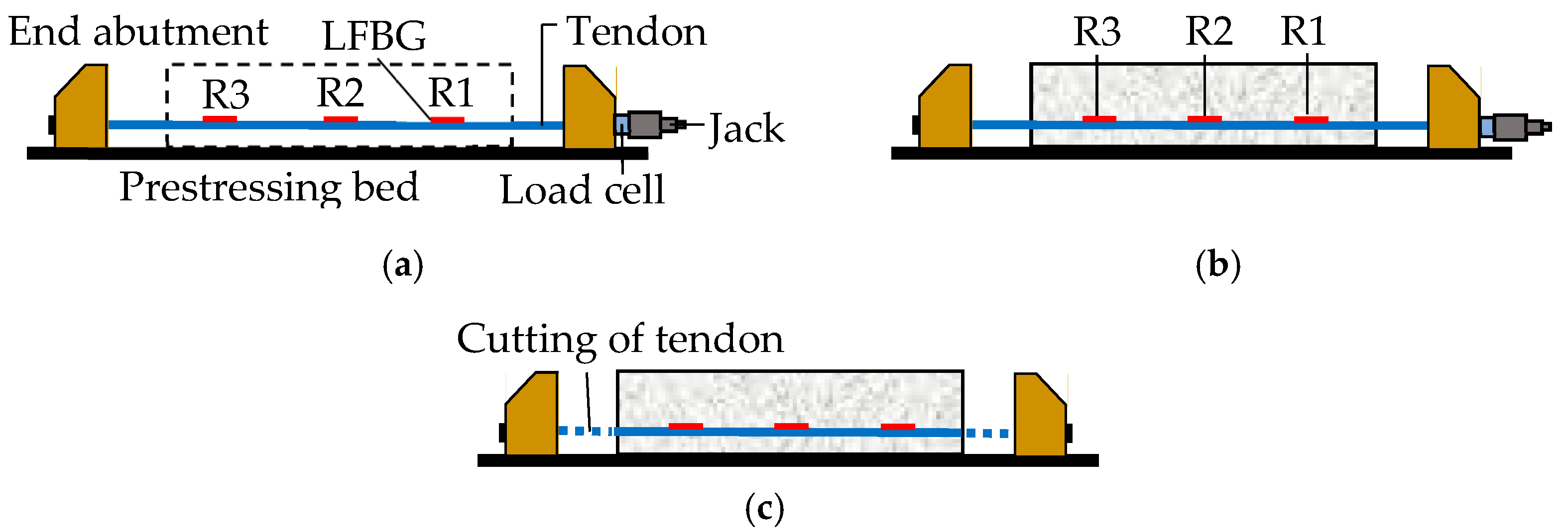
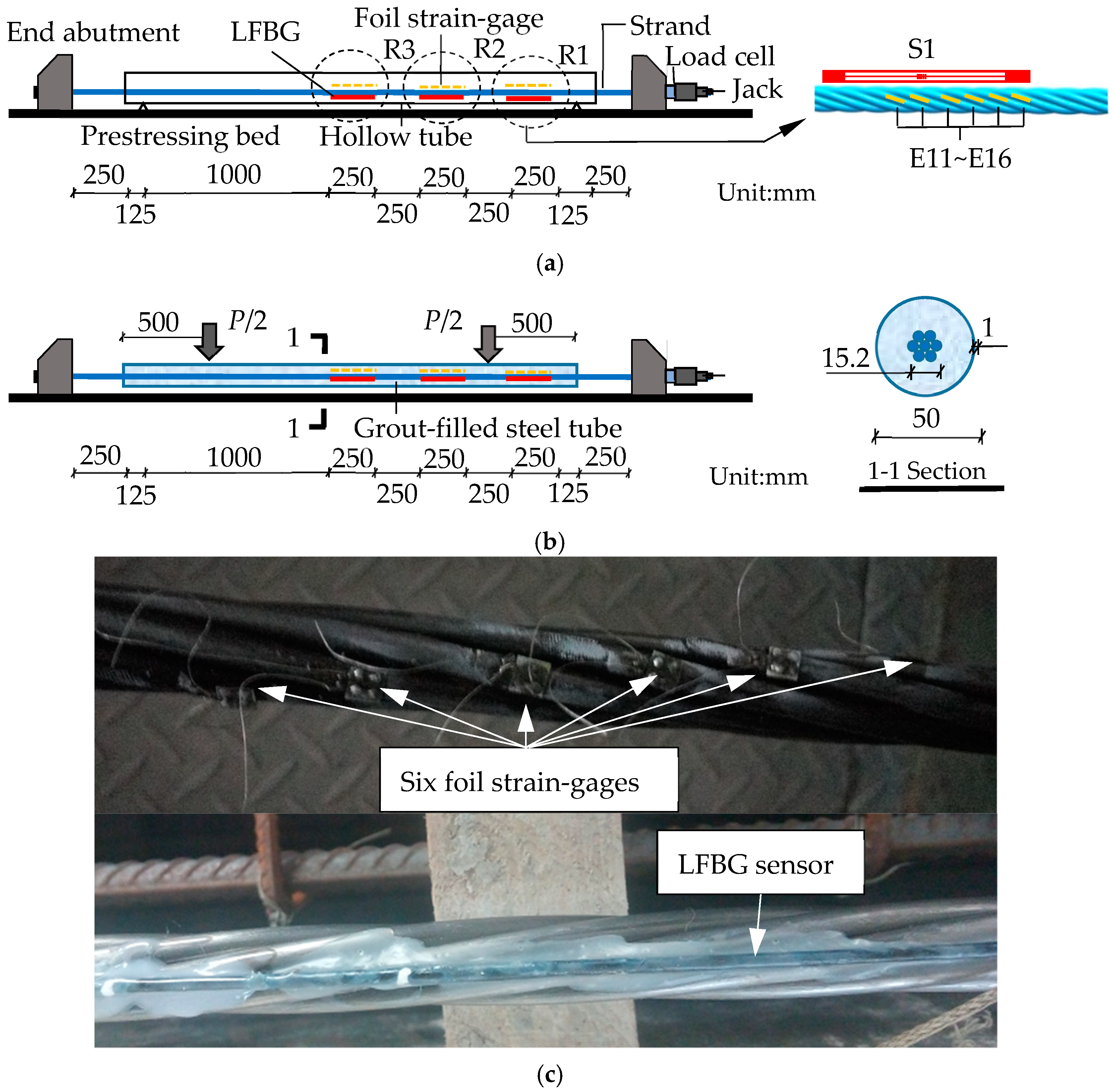
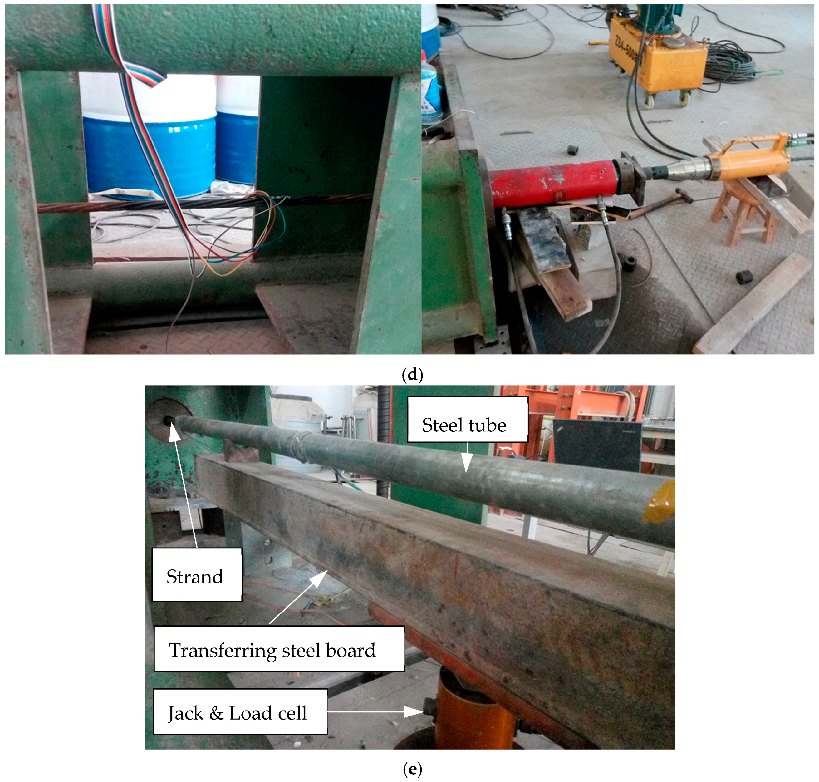
4.1. Pre-Tensioning Test

4.1.1. Test Design

As shown in Figure 7a, a 7-wire strand inserted into a hollow steel tube was fixed at both abutments of a prestressing bed. The tube was held by two supports and separated from the strand. The strand was placed at the center of the tube. The lengths of the strand and hollow steel tube were 3000 mm and 2500 mm, respectively. The nominal diameter and elastic modulus of the strand were 15.2 mm and 200 GPa, respectively. The outside and inside diameters of the hollow tube were 50 mm and 48 mm, respectively. Three monitored regions (R1–R3) with a uniform length of 250 mm were set from the right end to the mid-point of the strand, and the distance between adjacent regions was 250 mm. Three LFBG sensors (S1–S3) with a uniform gauge length of 250 mm were placed on R1–R3, respectively. In each region, each helical wire was attached to a foil strain-gauge (FSG) to measure the strain precisely. The numbering rule is as follows. For example, the 6 FSGs in R1 are named as E11–E16. The first number means the sensor is in R1 and the second number represents the number of the wire. Details are given in Figure 7c about the sensor placement on the wire.
The process of loading can be divided into three steps (Step I–III). At Step I, the increasing load F was applied by a jack to tension the strand through eight successive loading steps from 0 to 156 kN with an increment of 20 kN. After the final loading step, tensioning reduces from 156 kN to 149.8 kN because of the anchorage-seating loss and the loss due to draw-in of the wedge. At the beginning of Step II, the tube was filled with grout. When the strength of the grout exceeded 50 MPa (48 h after tensioning), the supports were removed. At Step III, a vertical load P was divided equivalently into two parts by a transferring steel board and applied at two points 500 mm away from both ends of the tube. P was increased with a loading step of 3 kN from 0 kN to 24 kN. Details about Step II and Step III are respectively shown in Figure 7b,d,e. The strains of R1–R3 in each helical wire at Steps I-III were measured by FSGs and LFBG sensors, respectively. In addition, the temperature was kept constant during the entire experiment to avoid the expansion or contraction of the abutments and strand. All measured data were updated by temperature compensation.

4.1.2. Results and Analysis

Table 1 gives the measured strains from the FSGs, the average values of the measured strains from the FSGs, and the measured strains from the LFBG sensors at Step I. Table 2 shows the comparison between the true stresses, the stresses calculated from the average values of the measured strains from the FSGs, and the stresses calculated from the strains obtained from the LFBG sensors. Four remarkable features are notable: First, most calculated stresses from sensor measurements are lower than the true stresses, the result ascribed to the gap between the adjacent wires. Second, the difference between the maximum and minimum strains of the six helical wires in the same region can approach or exceed 10% of the applied strain.
This result implies that the strain measured in one wire only does not necessarily represent the elongation of the whole strand. Moreover, the measured strains from the LFBG sensors are between the maximum and minimum strains from the FSGs and close to the average values of the measured strains from the FSGs. This result is attributed to the fact that LFBG can acquire the average elongation of six helical wires because the sensing part of the LFBG can cover the six wires.
Finally, most of the differences between the true stresses in the strand and the calculated stresses by strains from LFBG sensors are less than 5%. The maximum error is 6.0%. However, the differences between the true stresses in the strand and the calculated stresses from the average values of the measured strains from the FSGs are over 5%. The maximum error is up to 9.2%. It appears that the errors in strains from LFBG sensors are approximately half of those obtained from FSGs. An important reason behind this effect is that the FSGs attached on the helical wires are not parallel with the tensioning direction. In summary, these features show LFBG sensor is better suited to monitor prestress in the strand than common FSG.
Table 3 gives the monitored strains from different sensors at Step II. The comparison between the true stresses and the calculated stresses are shown in Table 4. Most of the losses calculated from the strains obtained from the LFBG sensors are approximate to or less than the corresponding losses calculated from the average values of the measured strains from the FSGs. Moreover, some FGSs become invalid at the end of this step. It further shows that the traditional electrical sensor may not satisfy the requirements of “local measurement in duct” due to the lack of long-term durability.
Before the beginning of Step III, the values of P, F, and sensors are set to zero again based on the measured data in Step II. The measured strains at each loading step of Step III are shown in Table 5. Note that the relationship between F and strand strains does not match Equation (1) anymore because the force is undertaken by not only strand but also solid grout and steel tube. There are two notable characteristics in Table 5. On the one hand, the number of damaged FSGs grows with increasing load. By contrast, all LFBG sensors can measure the strains well in the entire loading process. On the other hand, although the strains in R1–R3 should be close in theory, the difference between the measured strains from S1–S3 is less than 10% only in the case of P ≤ 12 kN. This phenomenon may be attributed to the crack in grout occurring near R1 and R2. The chief reason for that is when P = 12 kN, the measured strain is about 150 με, which is close to the threshold of the tensile strain of most concrete. This phenomenon shows the durability of LFBG sensors in the case of grout cracking in practical prestress monitoring.
Based on Equations (3)–(7), Table 6 lists the itemized prestress losses calculated from the monitored strains. Because the temperature was kept constant during the test, σl3 is zero. In addition, σl7 is zero because the strand was not cut. σl5 is also zero because the interval between grout curing and loading was short. Compared with the losses calculated from the average values of the measured strains from the FSGs, the losses calculated from the measured strains from the LFBG sensors were closer to the true losses. The error in the latter is only half of that in the former. This result verifies that LFBG sensor has more accuracy than traditional FSG in prestress monitoring.

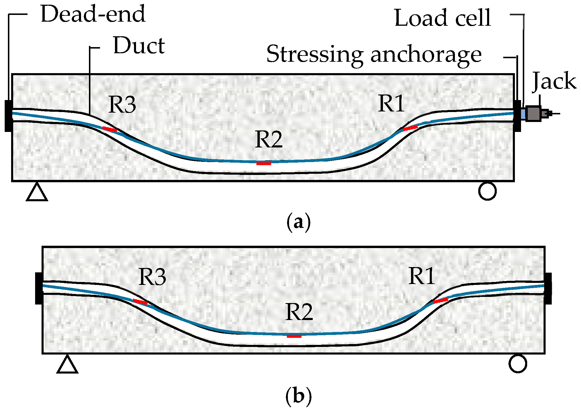
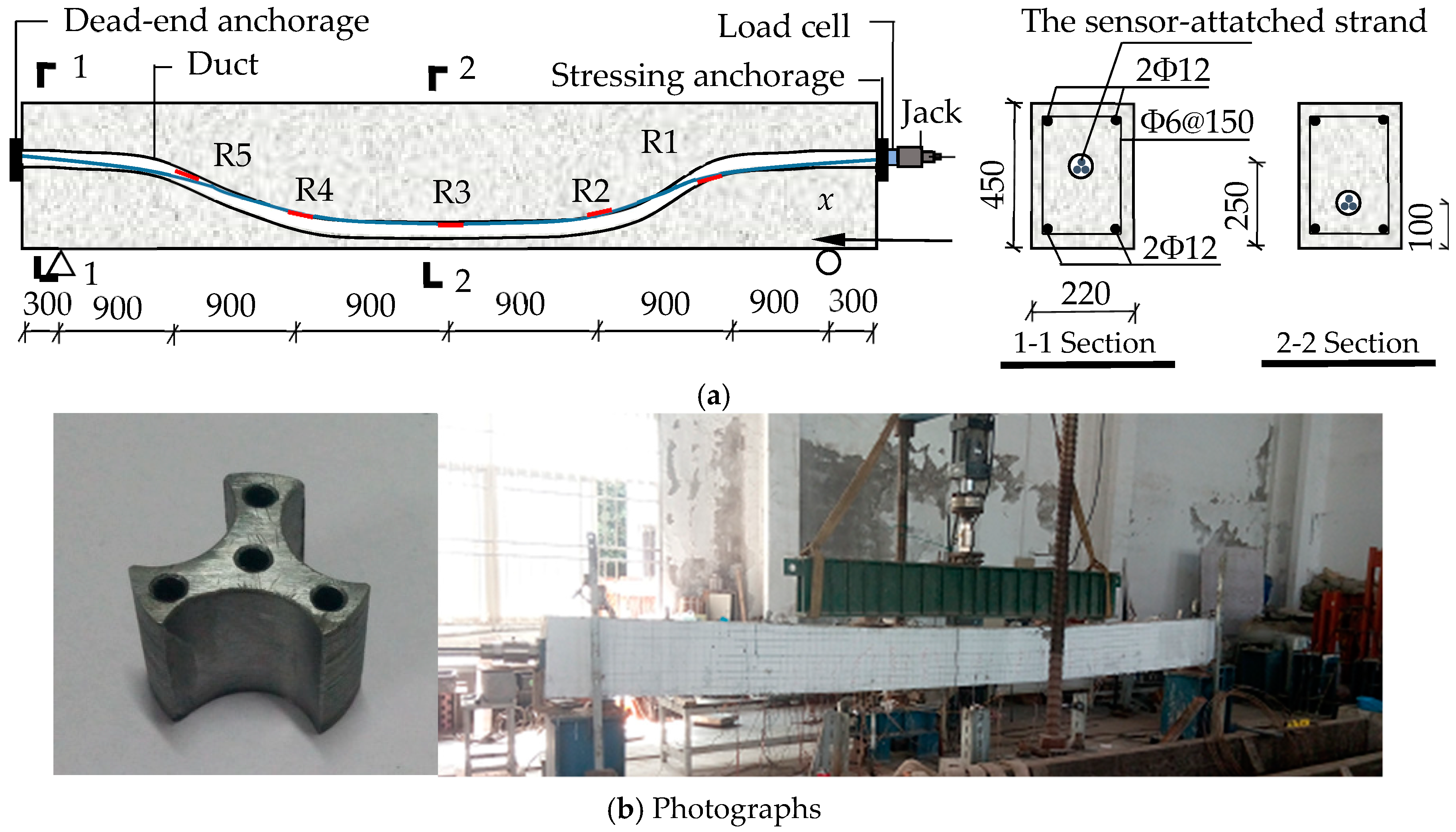
4.2. Post-Tensioning Test

4.2.1. Test Design

Details of the dimensions and reinforcement configuration of a simply-supported beam used in the experiment are shown in Figure 8a. The total length of the beam was 6000 mm, with a span of 5400 mm. The cross-section had a rectangular shape with 220 mm width and 450 mm depth. The compressive strength of the concrete was about 39 N/mm2. The elastic modulus and Poisson’s ratio of the concrete were 3.03 × 10⁴ N/mm2 and 0.19, respectively. A curved duct with a diameter of 50 mm was embedded into the beam. The process of the test can be divided into two steps (Step I–II). At Step I, a 3-strand tendon was passed through the duct and tensioned by the jack with an increasing load from 0 to 120, 240, 360, 480 and 540 kN. To counteract the frictional loss, we overloaded the final tension force to 555 kN that is 3% higher than 540 kN. Because of the effect of the anchorage-seating loss σl1, the tensioning force reduced from 555 kN to 426.6 kN in the case of anchoring. At Step II, it took 72 h to observe the steel relaxation and creep of the concrete and for the strength of grout to reach 50 MPa.
As shown in Figure 8a, we selected five regions located at the right linking point, 1/3 span, mid-span, 2/3 span, and left linking point (R1–R5) of the top strand for monitoring. Five LFBG sensors with a uniform gauge length of 250 mm were placed on R1–R5. 30 FSGs were successively attached on R1–R5 of the six helical wires of the strand. The numbering mode for the LFBG sensors and FSGs was the same as that in the last test. More details about the sensor installation and loading are illustrated in Figure 8b.

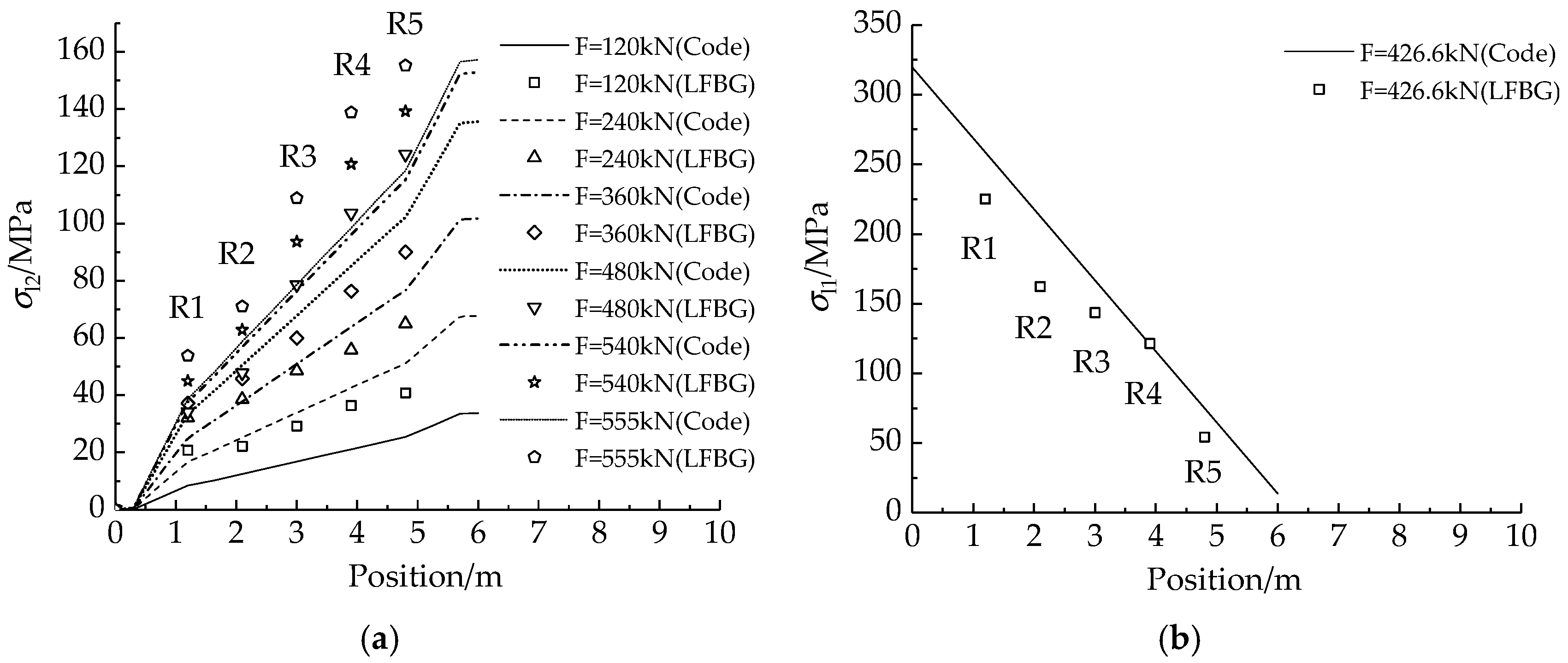
4.2.2. Results and Analysis

Different from the pre-tensioning case, the true stresses on R1–R5 cannot be obtained due to the frictional prestress loss distribution. Therefore, the theoretical prestress loss predictions by the Chinese Code [47] are used to replace the true prestress losses in the comparisons of σl2 and σl1. Table 7 gives the monitored strains from the FSGs and LFBG sensors at Step I. The differences between the maximum and minimum strains obtained from different wires also reaches or exceeds 10% of the applied strain. Assuming the average strain is approximate to the true strain, the large dispersion in the strain measurements demonstrates that the traditional short-gauge strain sensor is not suitable in prestress monitoring. Because the extending direction of the LFBG sensors is parallel to the tensioning force, most of the strains from LFBG sensor are larger than the average strains from FSG measurements at each loading step. This phenomenon also occurs in the previous test of pre-tensioning. Using Equation (9), Table 8 shows σl2 and σl1 calculated from LFBG sensor measurements at each loading step. Figure 9a,b show the comparisons between σl2 and σl1 calculated from the measured strains from the LFBG sensors and the theoretical predictions of prestress losses by the Chinese Code [47]. The developing trend of the calculated σl2 and σl1 are close to the loss profiles of theoretical predictions although there are some deviations between the calculated values and the predictions. This result also proves that the calculations for σl2 and σl1 are correct based on the strain measurements from the LFBG sensors.
At Step II, Table 9 lists the strain decrements of R1–R5 in 72 h due to (1) steel relaxation of the strands; (2) creep and shrinkage of the concrete. The sum of the corresponding prestress losses, σl4 and σl5, are listed in Table 10. Compared with the data in Table 4, the losses in Table 10 imply that the major parts of the losses are triggered by the creep and shrinkage of concrete. Also, several FSGs are observed to be invalid in this step owing to the immersion of grout. The fact that the FBG sensors can measure during 72 h of grout curing again shows the durability to the sensing part of the LFBG sensor.

5. Verification for the Prestress Loss Monitoring Using LFBG: In-Site Monitoring

The specific aims regarding in-site monitoring are to observe whether the LFBG sensors installed by the proposed installation procedure in Section 2.3 are valid in long-term monitoring, and to obtain the itemized prestress losses in practical post-tensioning to ensure the security of the construction.

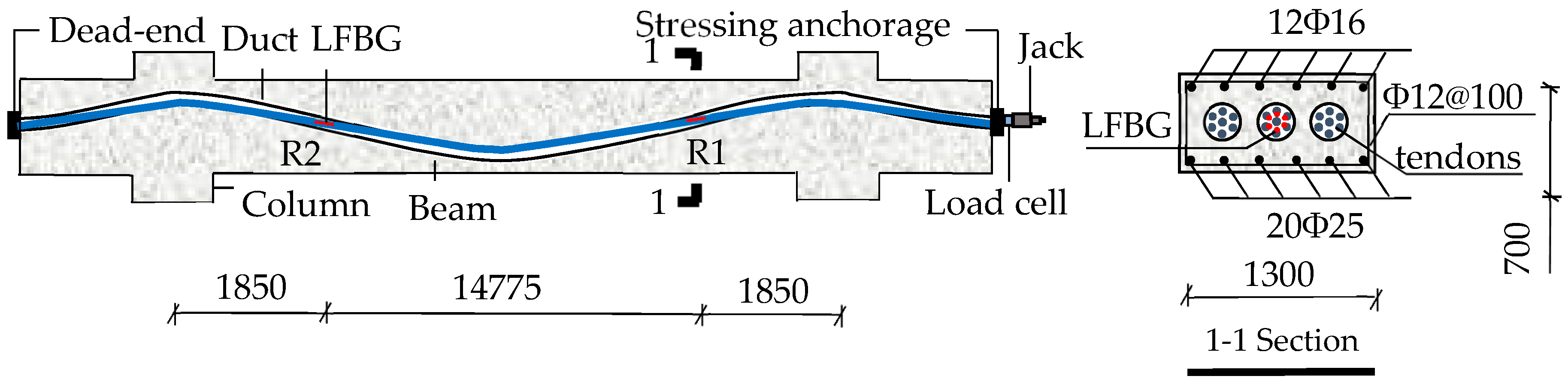
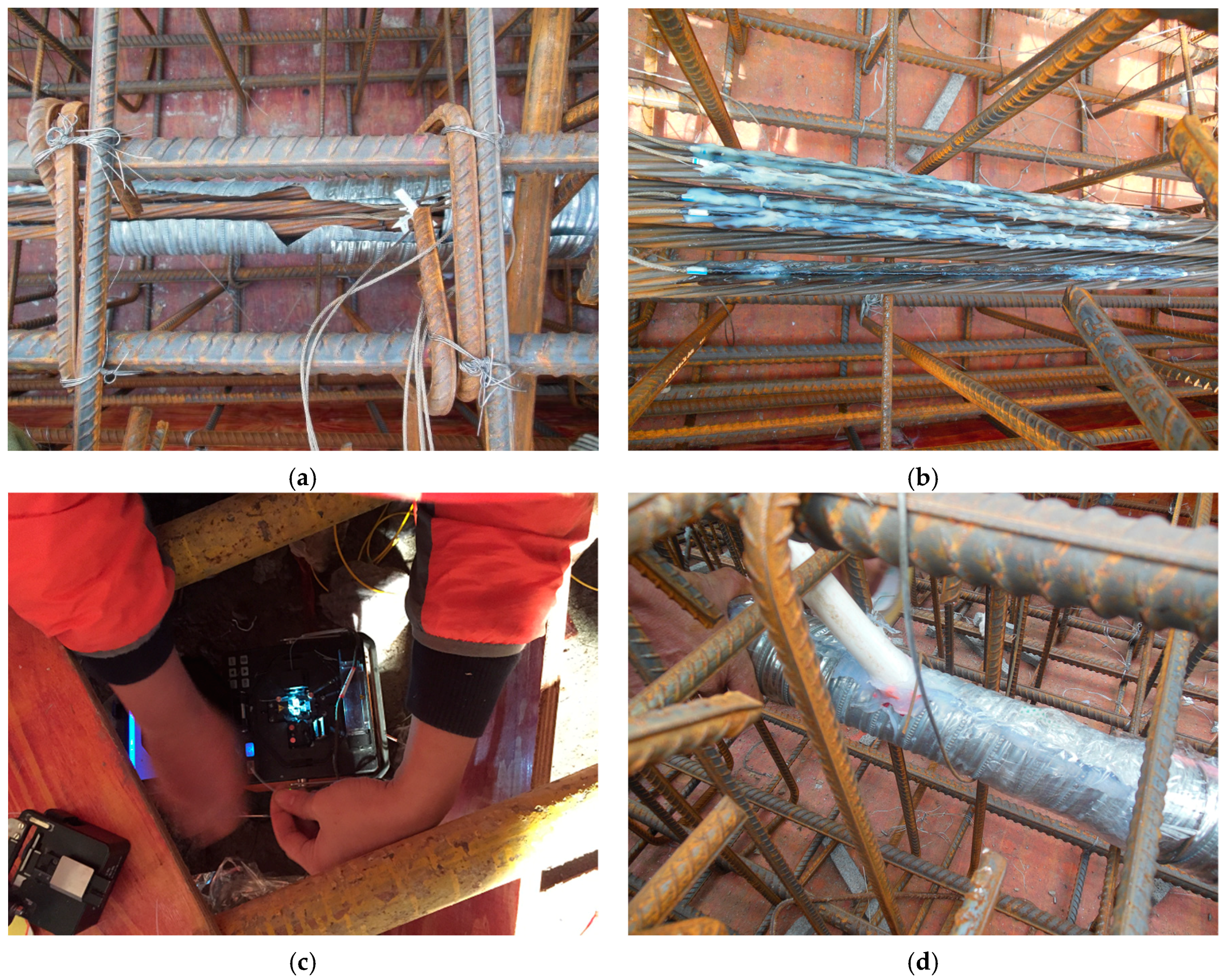
5.1. Member Fabrication and Sensor Placement

This practical prestress loss monitoring was based on the project of Multifunctional Drama Hall of the Fuzhou Straits Cultural Art Center in Fujian Province, China. The monitored beam had a length of 18.475 m. The width and the height of the beam were 1.3 m and 0.7 m, respectively. Details of the dimensions and reinforcement configuration are shown in Figure 10. Three 7-strand tendons were passed the curved duct, and all strands in three tendons had an identical nominal diameter of 15.2 mm. The ultimate tensile strength and elastic modulus of the strand were 1860 MPa and 200 GPa, respectively. The tensioning was controlled by the oil-pressure gauge of the jack used to apply tensioning to the tendons. There are three loading steps including 10 MPa, 20 MPa, and 28 MPa shown in the oil-pressure gauge to apply the prestresses of 358.40 MPa, 728.0 MPa, and 1023.7 MPa to the tendon, respectively. The applied prestress in the tendon at the final loading step contained an overstressing of 3% to counteract the frictional loss. Due to the anchorage-seating loss σl1, the applied prestress decreased from 1023.7 MPa to 862.3 MPa.
The six outer strands of the mid-tendon named as w1–w6 were used for prestress monitoring. As shown in Figure 10, two monitored regions were set nearby the linking points in the strands. 12 LFBG sensors were fixed in the regions. The numbering mode for the LFBG sensors is as follows. The six LFBG sensors on R1 of W1–W6 are named as S11–S16. The first number means the sensor is in R1, and the second number represents the number of the strand. The other six LFBG sensors on R2 of W1–W6 are named as S21–S26. At tensioning, the sensors measured the strain increments of each strand in each loading step. When the tensioning was finished, and the prestress began to transfer to the beam, the strain data were measured continuously. The entire monitoring lasted about 90 days, and all data were updated by temperature compensation.
Moreover, all LFBG sensors were installed by the installation method proposed in Section 2.3. Figure 11a–d show the whole process of sensor placement.

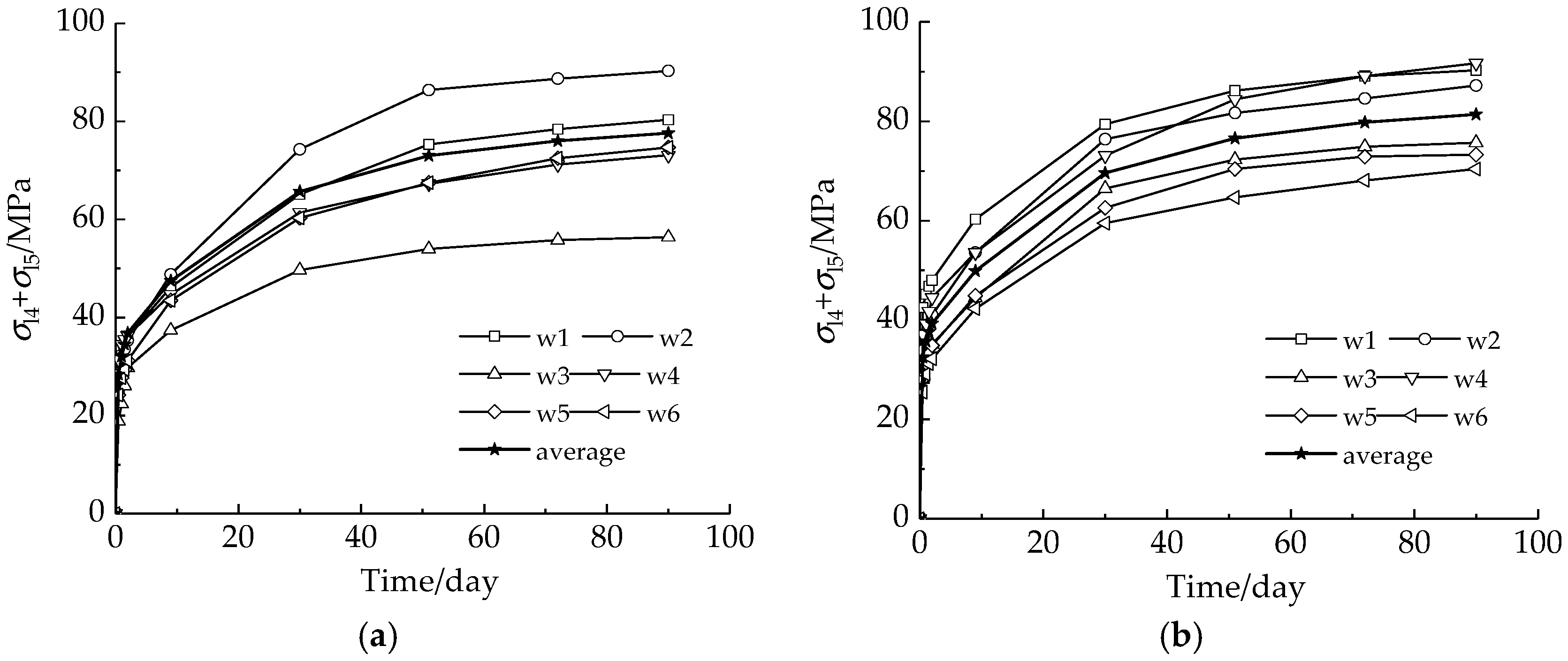
5.2. Results and Analysis

Table 11 lists the measured strains of the six helical strands and the average strains at each loading step in tensioning. The strains distributing in the strands are quite dispersed, and the deviation between the maximum and minimum strain can reach 50% of the average applied strains. This phenomenon implies that some strands such as w2 and w3 were still loose before the tensioning was applied. Moreover, the strand w1 may be ruptured earlier than other strands because it undertakes the extra prestress. Thus, a remarkable conclusion that can be derived from the data shown in Table 11 is that monitoring prestress in a tendon merely from the measured strains in one of the six helical wires using the traditional “short-gauge” strain sensor may ignore the uneven strain distribution in the same section. Table 12 and Table 13 give σl2 and σl1 calculated from the measured strains and their prediction based on the Chinese Code [47]. The fact that the calculated losses are close to the predictions implies that the prestress loss calculations are correct in principle based on the strain measurements from the LFBG sensors.
Table 13 records the strain reductions of W1–W6 due to steel relaxation of strands and creep of concrete in 90 days after anchoring. The calculated sum of the prestress losses, σl4 and σl5, is listed in Table 14 and illustrated in Figure 12.
There are three features that may be observed in Table 14 and Figure 12. First, the phenomenon that all LFBG sensors can trace the stress variation proves that the LFBG has enough durability for long-term prestress loss monitoring, and the proposed installation method is valid. Second, the increment of the sum of σl4 and σl5 in each strand has a similar trend. It proves the stability of the LFBG in measurements. Finally, almost 50% losses are completed in 48 h and the monitored data become stable after the 51st day. This feature shows that the prestress loss monitoring should be applied at an early stage of prestressing and last until the loss data tends to stabilize.

6. Conclusions

We demonstrated the deployment of the LFBG sensor for prestress loss monitoring and Evaluation. An appropriate length design of LFBG sensor and the installation method were proposed. Then we showed the calculation methods for the itemized prestress losses in pre-tensioning and post-tensioning. The applicability of the LFBG for prestress loss monitoring was verified by experiments in the laboratory and in-site monitoring. From the results and discussions, the following conclusions can be drawn:
(1)
An appropriate gauge length for LFBG sensor is at least 25 cm for prestress loss monitoring in the strand because the gauge can obtain the average strain by covering the six helical wires.
(2)
Severe frictions between the strand and duct and the grout crack can bring accidental damage to LFBG sensor. The proposed installation method can prevent the LFBG sensor from these ruptures effectively occurring at not only tendon tensioning but also structure loading. The durability and stability of the LFBG sensor are proved to be better than those of traditional FSGs.
(3)
The proposed calculation method acquired the itemized prestress losses at different stages of applying pretension accurately. Our results from the experiments including the cases of pre-tensioning and post-tensioning showed that the losses calculated from the measured strains of the LFBG sensors were more precise compared to those calculated from traditional FSGs. Moreover, from the in-site monitoring, we obtained the uneven stress distribution in different strands, measured the immediate losses at tensioning, and traced the time-dependent losses for 90 days. Thus, this calculation method can be easy to apply in the itemized prestress losses monitoring.
(4)
Compared with the traditional electrical sensor, the LFBG sensor is proved to have better durability for long-term prestress loss monitoring in practice, especially in the case of grout cracking and aggressive environment.

Author Contributions

The theoretical derivations were proposed by S.S. and D.H. The installation method was developed by Y.W. The experiments and in-site monitoring were designed and carried out by Z.-H.W. and X.G. The paper was revised and finalized by S.-L.M.

Funding

This work is supported by the National Natural Science Foundation of China (No. 51808119), the Technique Project of Fuzhou (Grant No. 2017-G-74), The Education and Scientific Research Project for Young and Middle-aged Teachers of Fujian Province (Grant No. JAT160044), the Transportation and Communication Science and Technology Project of Fujian Province (Grant No. 201536), the Major Research Projects of the Hebei Provincial Education Department(Grant No. ZD2015060) and the Open Fund of Fujian Provincial Key Laboratory of Advanced Technology and Informatization in Civil Engineering(Research on monitoring technology for prestress loss of steel strand in duct of building based on long gage fiber Bragg grating sensor).

Acknowledgments

The authors thank Zhi-ping Zhang and Yun-peng Zhang for their assistance with the experiments. The authors also express their gratitude for the anonymous reviewers for their constructive comments and suggestions.

Conflicts of Interest

The authors declare no conflict of interest.

References

  1. Nawy, E. Prestressed Concrete: A Fundamental Approach, 5th ed.; Pearson Education Asia Ltd.: Singapore; Chongqing University Press: Chongqing, China, 2006; pp. 59–81. [Google Scholar]
  2. Smith, J. Capacity of Prestressed Concrete Containment Vessels with Prestressing Loss; Sandia Report; Sandia National Laboratories: Albuquerque, NM, USA, 2001.
  3. Mo, Y.L.; Hwang, W.L. The effect of prestress losses on the seismic response of prestressed concrete frames. Comput. Struct. 1996, 59, 1013–1020. [Google Scholar] [CrossRef]
  4. Woodward, R.J.; Williams, F.W. Collapse of Ynys-y-Gwas Bridge, West Glamorgan. Proc. Inst. Civ. Eng. 1988, 84, 635–669. [Google Scholar] [CrossRef]
  5. Sumitro, S.; Jarosevic, A.; Wang, M.L. Elasto-magnetic sensor utilization on steel cable stress measurement. In Proceedings of the 1st Fib Congress, Osaka, Japan, 13–19 October 2002; pp. 13–19. [Google Scholar]
  6. Cho, K.; Park, S.Y.; Cho, J.R.; Kim, S.T.; Park, Y.H. Estimation of Prestress Force Distribution in the Multi-Strand System of Prestressed Concrete Structures. Sensors 2015, 15, 14079–14092. [Google Scholar] [CrossRef] [PubMed] [Green Version]
  7. Cappello, C.; Zonta, D.; Laasri, H.A.; Glisic, B.; Wang, M. Calibration of Elasto-Magnetic Sensors on In-Service Cable-Stayed Bridges for Stress Monitoring. Sensors 2018, 18, 466. [Google Scholar] [CrossRef] [PubMed]
  8. Chen, R.H.L.; Wissawapaisal, K. Application of Wigner-Ville Transform to Evaluate Tensile Forces in Seven-Wire Prestressing Strands. J. Eng. Mech. 2001, 127, 1206–1214. [Google Scholar] [CrossRef]
  9. Chen, R.H.L.; Wissawapaisal, K. An ultrasonic method for measuring tensile forces in a seven-wire prestressing strand. AIP Conf. Proc. 2002, 615, 1295. [Google Scholar] [CrossRef]
  10. Fang, Z.; Wang, J. Vertical prestressing loss in the bos girder of long-span PC continuous bridges. China Civ. Eng. J. 2006, 39, 78–84. [Google Scholar]
  11. Xiao, Y.; Zhang, Y.; Lu, J.; Liu, Y.; Cheng, W. Experimental analysis on pre-stress friction loss of crushed limestone sand concrete beams. Appl. Sci. 2018, 8. [Google Scholar] [CrossRef]
  12. Kim, J.T.; Yun, C.B.; Ryu, Y.S.; Cho, H.M. Identification of prestress-loss in PSC beams using modal information. Struct. Eng. Mech. 2004, 17, 467–482. [Google Scholar] [CrossRef]
  13. Kim, J.T.; Park, J.H.; Hong, D.S.; Cho, H.M.; Na, W.B. Vibration and impedance monitoring for prestress-loss prediction in PSC girder bridges. Smart Struct. Syst. 2009, 5, 81–94. [Google Scholar] [CrossRef]
  14. Ho, D.D.; Kim, J.T.; Stubbs, N.; Park, W.S. Prestress-force estimation in PSC girder using modal parameters and system identification. Adv. Struct. Eng. 2012, 15, 997–1012. [Google Scholar] [CrossRef]
  15. Yang, Y.; Myers, J.J. Prestress loss measurements in Missouri’s first fully instrumented HPC bridge. In Proceedings of the 84th Annual Meeting of the Transportation Research Board, Washington, DC, USA, 11–13 January 2005; pp. 1–19. [Google Scholar]
  16. Guo, X.; Liu, D.; Huang, P.; Zheng, X. Prestress loss of CFL in a prestressing process for strengthening RC beams. Int. J. Polym. Sci. 2017, 2017, 3832468. [Google Scholar] [CrossRef]
  17. Bartoli, I.; Salamone, S.; Phillips, R.; Scalea, F.L.; Sikorsky, C.S. Use of interwire ultrasonic leakage to quantify loss of prestress in multiwire tendons. J. Eng. Mech. 2011, 137, 324–333. [Google Scholar] [CrossRef]
  18. Ye, X.W.; Su, Y.H.; Xi, P.S. Statistical Analysis of Stress Signals from Bridge Monitoring by FBG System. Sensors 2018, 18, 491. [Google Scholar] [CrossRef]
  19. Xiao, F.; Chen, G.S.; Hulsey, J.L. Monitoring Bridge Dynamic Responses Using Fiber Bragg Grating Tiltmeters. Sensors 2017, 17, 2390. [Google Scholar] [CrossRef] [PubMed]
  20. Hu, D.T.; Guo, Y.X.; Chen, X.F.; Zhang, C.R. Cable Force Health Monitoring of Tongwamen Bridge Based on Fiber Bragg Grating. Appl. Sci. 2017, 7, 384. [Google Scholar] [CrossRef]
  21. Zhao, X.; Li, W.; Song, G.; Zhu, Z.; Du, J. Scour monitoring system for subsea pipeline based on active thermometry: Numerical and experimental studies. Sensors 2013, 13, 1490–1509. [Google Scholar] [CrossRef] [PubMed]
  22. Kong, X.; Ho, S.C.M.; Song, G.; Cai, C.S. Scour Monitoring System Using Fiber Bragg Grating Sensors and Water-Swellable Polymers. ASCE J. Bridge Eng. 2017, 22, 04017029. [Google Scholar] [CrossRef]
  23. Li, W.; Ho, S.C.M.; Song, G. Corrosion detection of steel reinforced concrete using combined carbon fiber and fiber Bragg grating active thermal probe. Smart Mater. Struct. 2016, 25, 045017. [Google Scholar] [CrossRef] [Green Version]
  24. Li, W.; Xu, C.; Ho, S.C.M.; Wang, B.; Song, G. Monitoring concrete deterioration due to reinforcement corrosion by integrating acoustic emission and FBG strain measurements. Sensors 2017, 17, 657. [Google Scholar] [CrossRef] [PubMed]
  25. Hou, Q.; Ren, L.; Jiao, W.; Zou, P.; Song, G. An improved negative pressure wave method for natural gas pipeline leak location using FBG based strain sensor and wavelet transform. Math. Probl. Eng. 2013, 2013, 278794. [Google Scholar] [CrossRef]
  26. Ho, S.C.M.; Ren, L.; Li, H.N.; Song, G. A fiber Bragg grating sensor for detection of liquid water in concrete structures. Smart Mater. Struct. 2013, 22, 055012. [Google Scholar] [CrossRef]
  27. Hou, Q.; Jiao, W.; Ren, L.; Cao, H.; Song, G. Experimental study of leakage detection of natural gas pipeline using FBG based strain sensor and least square support vector machine. J. Loss Prev. Process. Ind. 2014, 32, 144–151. [Google Scholar] [CrossRef]
  28. Feng, Q.; Kong, Q.; Huo, L.; Song, G. Crack detection and leakage monitoring on reinforced concrete pipe. Smart Mater. Struct. 2015, 24, 115020. [Google Scholar] [CrossRef]
  29. Kim, J.M.; Kim, H.W.; Park, Y.H.; Yang, I.H.; Kim, Y.S. FBG sensors encapsulated into 7-wire steel strand for tension monitoring of a prestressing tendon. Adv. Struct. Eng. 2012, 15, 907–917. [Google Scholar] [CrossRef]
  30. Kim, S.T.; Park, Y.H.; Park, S.Y.; Cho, K.; Cho, J.R. A Sensor-Type PC Strand with an Embedded FBG Sensor for Monitoring Prestress Forces. Sensors 2015, 15, 1060–1070. [Google Scholar] [CrossRef] [PubMed] [Green Version]
  31. Cho, K.; Kim, S.T.; Cho, J.R.; Park, Y.H. Estimation of tendon force distribution in prestressed concrete girders using smart strand. Appl. Sci. 2017, 7, 1319. [Google Scholar] [CrossRef]
  32. Shin, K.J.; Lee, S.C.; Kim, Y.Y.; Kim, J.M.; Park, S. Construction condition and damage monitoring of post-Tensioned PSC girders using embedded sensors. Sensors 2017, 17, 1843. [Google Scholar] [CrossRef] [PubMed]
  33. Kim, J.M.; Kim, C.M.; Choi, S.Y.; Lee, B.Y. Enhanced strain measurement range of an FBG sensor embedded in seven-wire steel strands. Sensors 2017, 17, 1654. [Google Scholar] [CrossRef] [PubMed]
  34. Zhou, Z.; He, J.; Chen, G.; Ou, J. A smart steel strand for the evaluation of prestress loss distribution in post-tensioned concrete structures. J. Intell. Mater. Syst. Struct. 2009, 20, 1901–1912. [Google Scholar] [CrossRef]
  35. Lan, C.; Zhou, Z.; Ou, J. Full-scale prestress loss monitoring of damaged RC structures using distributed optical fiber sensing technology. Sensors 2012, 12, 5380–5394. [Google Scholar] [CrossRef] [PubMed]
  36. Zhang, H.; Wu, Z.S. Performance evaluation of BOTDR-based distributed fiber optic sensors for crack monitoring. Struct. Health Monit. 2008, 7, 143–156. [Google Scholar] [CrossRef]
  37. Zhang, H.; Wu, Z.S. Performance Evaluation of PPP-BOTDA-Based Distributed Optical Fiber Sensors. Int. J. Distrib. Sens. Netw. 2012, 2012, 414692. [Google Scholar] [CrossRef]
  38. Mckeeman, I.; Fusiek, G.; Perry, M.; Johnston, M.; Saafi, M.; Niewczas, P.; Walsh, M.; Khan, S. First-time demonstration of measuring concrete prestress levels with metal packaged fibre optic sensors. Smart Mater. Struct. 2016, 25, 095051. [Google Scholar] [CrossRef]
  39. Perry, M.; Yan, Z.; Sun, Z.; Zhang, L.; Niewczas, P.; Johnston, M. High Stress monitoring of prestressing tendons in nuclear concrete vessels using fiber optic sensors. Nucl. Eng. Des. 2014, 268, 35–40. [Google Scholar] [CrossRef]
  40. Majda, P.; Skrodzewicz, J. A modified creep model of epoxy adhesive at ambient temperature. Int. J. Adhes. Adhes. 2009, 29, 396–404. [Google Scholar] [CrossRef]
  41. Li, E.; Xi, J.; Chicharo, J.F.; Liu, T.; Li, X.; Jiang, J.; Li, L.; Wang, Y.; Zhang, Y. The Experimental evaluation of FBG sensor for strain measurement of prestressed steel strand. In SPIE Smart Structures, Devices, and Systems II; SPIE: Bellingham, WA, USA, 2005; Volume 5649, pp. 463–469. [Google Scholar]
  42. Li, S.; Wu, Z. Development of distributed long-gage fiber optic sensing system for structural health monitoring. Struct. Health Monit. 2007, 6, 133–145. [Google Scholar] [CrossRef]
  43. Wu, Z. Durability Study of Fiber Bragg Grating Strain Sensor Packaged with Fiber in Structural Health Monitoring. Master’s Thesis, Southeast University, Nanjing, China, 27 May 2013. [Google Scholar]
  44. Hong, W.; Wu, Z.S.; Yang, C.Q.; Wan, C.; Wu, G. Investigation on the damage identification of bridges using distributed long-gauge dynamic macrostrain response under ambient excitation. J. Intell. Mater. Syst. Struct. 2012, 23, 85–103. [Google Scholar] [CrossRef]
  45. Wang, T.; Tang, Y.S. Dynamic displacement monitoring of flexural structures with distributed long-gage macro-strain sensors. Adv. Mech. Eng. 2017, 9. [Google Scholar] [CrossRef] [Green Version]
  46. Tang, Y.S.; Ren, Z.D. Dynamic Method of Neutral Axis Position Determination and Damage Identification with Distributed Long-Gauge FBG Sensors. Sensors 2017, 17, 411. [Google Scholar] [CrossRef] [PubMed]
  47. Ministry of Housing and Urban-Rural Development of the People’s Republic of China. Code for Design of Prestressed Concrete Structures; China Architecture & Building Press: Beijing, China, 2016.
Figure 1. The structural design of the packaged LFBG sensor proposed by Li [42].
Sensors 18 04106 g001
Figure 2. Comparison of gauge length between LFBG sensor and the short-gauge sensor.
Sensors 18 04106 g002
Figure 3. Sketches of the restraining block for (a) 7-strand tendon; (b) 3-strand tendon; and (c) for separating adjacent strands.
Sensors 18 04106 g003
Figure 4. The installation procedure of the LFBG sensor. (a) Place the strands through the marked pipe; (b) strip the partial corrugated pipe; (c) install the restraining blocks; (d) attach the LFBG sensors; (e) connect the sensor to the optical cable; and (f) connect the protection sleeve.
Sensors 18 04106 g004
Figure 5. Three stages of pre-tensioning: (a) applying prestress to tendons; (b) casting and curing of concrete member; and (c) cutting of tendon.
Sensors 18 04106 g005
Figure 6. The schematic of the two stages of post-tensioning: (a) Application of tensioning to tendons; and (b) Fitting the wedge and cutting the tendon.
Sensors 18 04106 g006
Figure 7. The sketches and photographs of the test design: (a) applying tensioning to the bare strand; (b) applying load on the cement-filled steel tube; (c) the photograph of the strand attached with sensor; (d) the photograph of tensioning and (e) the photograph of vertical load applied on the cement-filled steel tube.
Sensors 18 04106 g007aSensors 18 04106 g007b
Figure 8. Sketches and photographs of the experiment. (a) Applied tensioning to tendons; and (b) photographs of the restraining block and tensioning.
Sensors 18 04106 g008
Figure 9. The comparisons of the two calculated losses and the predictions according to the Chinese Code [44]: (a) σl2; and (b) σl1.
Sensors 18 04106 g009
Figure 10. The schematic of the monitored beam in in-site measurement.
Sensors 18 04106 g010
Figure 11. Photographs of the LFBG sensor deployment in in-site monitoring: (a) Peeling the marked region to expose the tendon; (b) attaching the LFBG sensors on the strands; (c) connecting the sensor to the optical cable; and (d) connecting the protection sleeve to the pipe.
Sensors 18 04106 g011
Figure 12. The increment of the sum of σl4 and σl5 for 90 days: (a) R1; and (b) R2.
Sensors 18 04106 g012
Table 1. The monitored strains of the strand at Step I. (Unit: με).
RegionF/kN20406080100120140156149.8
R1E1181714872189287935404201479152465053
E1252010421656233130453734440050134708
E1372013141971267033363978458351244936
E1467112911979268233814055469252445080
E1579515762305301437074374500655505271
E1671613482028271433934044466552145095
Average strain(FSG) *70713432021271534004064468952325024
S171314262129280835244237494054825270
R2E2169513532013267433563991459351564929
E2261612541903255332313857445250044725
E2375314202076272834104035463151844976
E2461612111825245631363753434948924684
E2570513852062274034604105472752795149
E2668713291973261633023911450050314828
Average strain(FSG)67813251975262833163942454250914882
S268513882035277634254077481452385028
R3E3170713822080276033844060471652365014
E3268313592063275633914073473952655044
E3370513181959259231873824445649464826
E3473714252129282034654135480153084986
E3562112982004269833504020469052024979
E3669413792090278834474120480053075082
Average strain(FSG)69113602054273633714039470052114989
S371114072064276435004186490053565128
* Average strain (FSG) represents the average value of the strains from the six FSGs obtained from the same region.
Table 2. The measurement errors in calculated stresses from the strains obtained from the FSGs and LFBG sensors.
F/kN20406080100120140156149.8
True Stress/MPa143.0285.7428.6571.4714.3857.11000.01114.31070.0
R1Stress(FSG) */MPa141.4268.6404.2543.0680.0812.8937.81046.41004.8
Error/%−1.1−6.0−5.7−4.8−4.6−6.2−5.9−6.1−6.1
Stress(LFBG) **/MPa142.6285.2425.8561.6704.8847.4988.01096.41054.0
Error/%−0.3−0.2−0.7−1.7−1.3−1.1−1.2−1.6−1.5
R2Stress(FSG)/MPa135.6265.0395.0525.6663.2788.4908.41018.2976.4
Error/%−5.0−7.3−7.8−8.0−7.2−8.0−9.2−8.6−8.7
Stress(LFBG)/MPa137.0277.6407.0555.2685.0815.4962.81047.61005.6
Error/%−4.0−2.8−5.0−2.8−4.1−4.9−3.7−6.0−6.0
R3Stress(FSG)/MPa138.2272.0410.8547.2674.2807.8940.01042.2997.8
Error/%−3.5−4.8−4.2−4.2−5.6−5.8−6.0−6.5−6.7
Stress(LFBG)/MPa142.2281.4412.8552.8700837.2980.01071.21025.6
Error/%−0.6−1.5−3.7−3.3−2.3−1.9−2.0−3.9−4.1
* Stress (FSG) is the stress calculated from the average strain (FSG) in Table 1. ** Stress (LFBG) is the stress calculated from the measured strains by LFBG sensors in Table 1.
Table 3. The monitored strains of the strand at Step II. (Unit: με).
Time/Hour0123122448
F/KN149.8149.55149.35149.24149.1148.95148.9
R1E115053504650405038503250155009
E124708469746894685467446624656
E1349364928492149204918--
E145080506650615058504450275022
E155271526552615257524952345226
E165095508750815077506850525044
Average strain of E11–E165024501550095006499849984991
S15270526052535249524252385234
R2E214929491849094904489348804865
E2247254720471747154709 -
E234976496749604958495149314909
E244684467346664662465746334624
E255149514351385135513051135094
E264828482048144810480147774764
Average strain of E21–E264882487448674864485748674851
S25028501950135009500349974995
R3E315014500549974993498949834980
E325044503350255018500850055002
E334826481748104808480147994795
E344986497849724970496749574951
E35497949714964496149574952-
E365082507050635058505450485044
Average strain of E31–E364989497949724968496349574954
S35128511751125108510350975094
Table 4. The stresses and the measurement errors calculated from the strains obtained from the FSGs and LFBG sensors.
Time/Hour123122448
True stress/MPa1.783.24.05.06.076.43
R1Stress(FSG)/MPa1.833.65.25.26.6
Error/%1.1−6.3−10.04.04.02.6
Stress(LFBG)/MPa23.44.25.66.47.2
Error/%12.46.35.012.05.412.0
R2Stress(FSG)/MPa1.633.6536.2
Error/%−10.1−6.3−10.0050.5−3.6
Stress(LFBG)/MPa1.833.856.26.6
Error/%1.1−6.3−5.002.12.6
R3Stress(FSG)/MPa23.44.25.26.47
Error/%12.46.35.04.05.48.9
Stress(LFBG)/MPa2.23.2456.26.8
Error/%23.60002.15.8
Table 5. The monitored strains of the strand at Step III. (Unit: με).
P/kN3691215182124
F/kN0.62.25.810.115.120.826.732.7
R1E11144689145230318--
E121663105155258376516682
E13--------
E1463473123----
E151448103-----
E1684288153233---
Average strain(FSG)124792144240347516682
S1124797155252367508662
R2E2163275130195279379482
E22--------
E23114995150231315--
E24114392141221312425551
E251959118172----
E262266116174260365--
Average strain(FSG)145099153227318402517
S2114793149234335456578
R3E3184491141206275373480
E32145098157236---
E3394281122----
E341961------
E35--------
E3663374124196273384-
Average strain(FSG)114686136213274379480
S3124289141211297396500
Table 6. Comparison of different prestress losses in the pre-tensioning experiment.
Itemized Prestress Lossσl1 + σl2, IIσl2, Iσl3σl4σl5σl6σl7Total Loss
True loss/MPa44.3- *06.40 **-050.7
Loss(FSG)Value/MPa41.6-06.60-048.2
Error/%−6.1-03.10-0−4.9
Loss(LFBG)Value/MPa42.4-06.90-049.3
Error/%−4.3-07.80-0−2.8
* “-” denotes this loss does not exist in pre-tensioning case. ** “0” denotes that σl5 is small because the interval between grout curing and loading is short.
Table 7. The monitored strains of the strand at Step I. (Unit: με).
F/kN120240360480540555426.6
R1E111371277541935682636864715214
E121336270441115532621863435111
E131300262539935368604661714807
E141257254337865250584659544968
E151325268941615504624363685125
E161382280042295686637164945227
Average strain(FSG)1329268940795504618263005075
S11321268940895529620063365211
R2E211357272941795589628964215546
E221318265740795471613262645439
E231264255438965250593260755271
E241236250438075154582559365154
E251289260640065392607962325451
E261361272142045500623663965496
Average strain(FSG)1304262940295393608262215393
S21314265740465461611162505439
R3E311321269341255461615062615461
E321296263940465354603661465375
E331254257938935200589660005246
E341229247538295161568658715164
E351243257539505236587559795229
E361351270741155456614262615432
Average strain(FSG)1282261139935311596460865318
S31279260739755307595760615343
R4E411282264640255321598660825404
E421279262940365318600761075421
E431204253637935039564657965129
E441189241437435036557956545079
E451218256838715161580758895275
E461329272140575432611462155575
Average strain(FSG)1250258639215218585759575314
S41243257138935182582159115304
R5E511236238938615246581459715689
E521246255039365150576158645618
E531186252539005089572158615518
E541182250737895029565057895554
E551150240432574618519352615018
E561286268940975254597560965731
Average strain(FSG)1214251138075064568658075521
S51221252538255079572958295557
Table 8. σl2 and σl1 calculated from the strains of the LFBG sensors at Step I. (Unit: MPa).
Itemized Lossesσl2σl1
P/kN120240360480540555426.6
0 *------305.7
R120.832.237.234.245.053.8225.0
R222.238.645.847.862.871.0162.2
R329.248.660.078.693.6108.8143.6
R436.455.876.4103.6120.8138.8121.4
R540.865.090.0124.2139.2155.254.4
* “0” is the zero point in the coordinate that represents the right end of the beam in Figure 8a.
Table 9. The results of strain measurement from various sensors at Step II. (Unit: με).
Time/Hour12312244872
RR1E115130511151025052503349994976
E125016498849764923489548624853
E134713468746724609457045444542
E144888486848534790477747524738
E155038501250054955492748994876
E165129509750905021499349554949
Average strain(FSG)4985496049494891486548354822
S15141512151135056502649874970
RR2E215450542354115338532953025275
E225348532253095256523152025183
E235182515651375085505750305006
E245068504850394980496349324905
E255362533253175272525652185197
E265402538253775313529352525248
Average strain of E21–E265302527752665208518951565136
S25366534053245251522351985184
RR3E31540753905377531953105282-
E325319529552765245520951805166
E335184516251435097507650445022
E34511450975091504150174986-
E355175515451445100508250495029
E365377535853505298528752665246
Average strain of E31–E365263524352305183516451355116
S35266524152315167515551315118
RR4E415309528352705210517451515126
E425321529052815218518151555121
E435035501150044946490748834848
E444991497749644909487648514825
E4551845152- - - - -
E465484545454315371534653195271
Average strain of E41–E465221519551905131509750725038
S45215519151805108507050214999
RR5E515580554455295451543053925375
E525519550754915447541153805345
E53542254065387531052815252-
E5454545423- - - - -
E554914487848694808477147364712
E565631559255655562554455045479
Average strain of E51–E565420539253685316528752535228
S55459543254075363532352715239
Table 10. The sum of σl4 and σl5 calculated from the strains obtained from the LFBG sensors. (Unit: MPa).
Itemized Lossesσl4+ σl5
Time/hour12312244872
0 *17.321.726.135.742.145.346.3
R114.018.019.631.037.044.848.2
R214.619.823.037.643.248.251.0
R315.420.422.435.237.642.445.0
R417.822.624.839.246.856.661.0
R519.625.030.038.846.857.263.6
* “0” is the zero point in the coordinate that represents the right end of the beam in Figure 8a.
Table 11. The monitored strains of the strands at tensioning. (Unit: με).
Applied Stress/MPa358.4728.01023.7862.3
R1S112456493867556196
S121320306742543606
S131428294143253972
S141621346149884298
S151913391154954805
S162066363850914611
Average strain of S11–S161801365951514581
R2S212361470565686561
S221074253236433628
S23759177130032977
S241945383251625151
S251888360951525134
S262027389849494931
Average strain of S21–S261676339147464730
Table 12. σl2 and σl1 calculated from the strains of the LFBG sensors. (Units: MPa).
Itemized Prestress Lossesσl2σl1
Applied stress358.4728.01023.7862.3
R1w1−120.5−234.9−293.5109
w2101.0129.9194.2126.3
w379.9154.5180.368.9
w442.353.151.0134.6
w5−14.6−34.6−47.8134.5
w6−44.518.431.093.6
Average(LFBG) *7.314.419.2111.2
Prediction(Code) **7.916.022.5108.4
R2w1−102.0−189.5−257.11.4
w2149.0234.3313.32.9
w3210.4382.7438.15.1
w4−20.9−19.217.12.2
w5−9.824.219.13.5
w6−36.9−32.158.63.6
Average(LFBG) *31.666.798.23.1
Prediction(Code) **29.459.783.90
* represents the average stresses or prestress losses calculated from strains obtained from the LFBG sensors. ** the values are estimated based on the Chinese Code [47].
Table 13. The monitored strains of the strands at the in-service stage. (Unit: με).
TimeR1R2
W1W2W3W4W5W6AverageW1W2W3W4W5W6Average
061963606397242984805461145816561362829775151513449314730
12 h60523461387541374681440944366343345428334961499048004564
24 h60313443385741214663438744176329343628154950497347824548
36 h60203434383841164654436344046321342728064937496447714538
48 h60113425381941124645434443936315341827974923495547664529
9 days59593356378040694582428043386252335327494876490447144475
30 days58623225371739834496418342446154323626364776481346264374
51 days58103163369539534459416442076119320926064718477345994337
72 days57943151368639334433415241926104319425934694476045824321
90 days57843143368339234422414641836098318125894681475845704313
Table 14. The sum of σl4 and σl5 calculated from the strains obtained from the LFBG sensors. (Units: MPa).
TimeR1R2
W1W2W3W4W5W6AverageW1W2W3W4W5W6Average
12 h28.128.318.931.424.239.428.442.533.928.137.128.125.532.5
24 h32.231.822.434.527.743.732.145.237.431.639.231.429.135.7
36 h34.333.526.135.529.448.434.546.839.233.341.733.231.237.6
48 h36.135.329.836.331.252.136.848.041.035.144.534.932.239.3
9 days46.248.837.444.743.564.547.560.353.644.553.644.942.349.9
30 days65.174.349.761.460.383.565.779.476.466.573.162.659.569.6
51 days75.386.45467.367.587.273.086.281.772.384.470.464.776.6
72 days78.488.755.871.272.589.576.089.184.674.989.172.968.179.8
90 days80.390.356.473.174.790.777.690.387.275.791.773.370.481.4

