Accurate Determination of the Q Quality Factor in Magnetoelastic Resonant Platforms for Advanced Biological Detection

Abstract

The main parameters of magnetoelastic resonators in the detection of chemical (i.e., salts, gases, etc.) or biological (i.e., bacteria, phages, etc.) agents are the sensitivity $S$ (or external agent change magnitude per Hz change in the resonance frequency) and the quality factor $Q$ of the resonance. We present an extensive study on the experimental determination of the $Q$ factor in such magnetoelastic resonant platforms, using three different strategies: (a) analyzing the real and imaginary components of the susceptibility at resonance; (b) numerical fitting of the modulus of the susceptibility; (c) using an exact mathematical expression for the real part of the susceptibility. $Q$ values obtained by the three methods are analyzed and discussed, aiming to establish the most adequate one to accurately determine the quality factor of the magnetoelastic resonance.

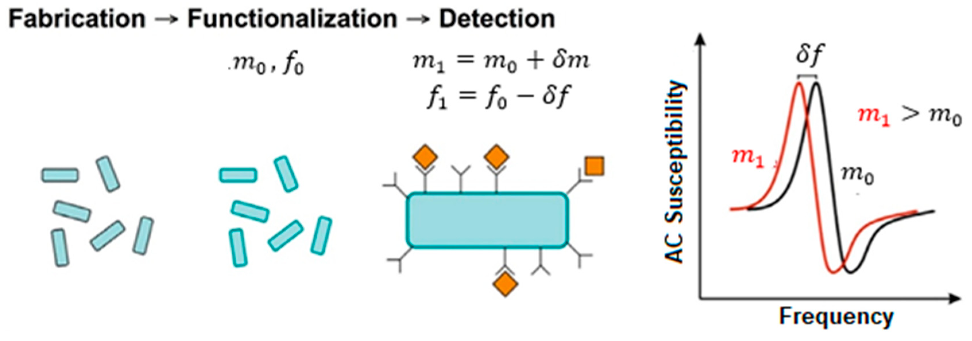
1. Introduction

Magnetoelastic resonators used as sensing devices present advantages like allowing remote “query and answer” [1,2] as well as low cost and low power consumption [3]. Due to these reasons, chemical and many other parameters can be detected: aqueous chemicals including pH [1], salt, and glucose concentrations [3], as well as inorganic salt depositions [4], gas humidity [5], gases such as carbon dioxide [6], or toxic volatile organic compounds (VOCs) such as benzene or hexane, among others [7]. In recent years, they have become a hot topic as novel wireless biosensors for bacteria, potentially lethal for humans, such as Salmonella [8,9], Bacillus anthracis [9], or Escherichia coli [10]. Such detection will be achieved if the surface of the magnetoelastic resonator is coated with an appropriate smart functionalized film that interacts with the target of interest.

The detection process in such sensors is based on the shift of the magnetoelastic resonance (MER) frequency under the action of an external agent, easily seen when measuring the magnetic susceptibility versus the frequency of the applied magnetic field. In the case of biological agents, the adhesion of different bacteria to the resonators causes an increase in the total mass, which leads to a decrease in the MER (see Figure 1).

Among the magnetoelastic materials to be used as biological sensors, Fe-based amorphous ferromagnetic alloys in the form of a ribbon are among the most suitable, mainly due to their high magnetoelastic coupling coefficient ($k$), high saturation magnetostriction (${\lambda }_S$), and high saturation magnetization ($M_S$) [11].

The good performance of a magnetoelastic sensing device is mainly determined by two parameters: sensitivity and quality factor. The sensitivity is related to the lowest detectable frequency change. This depends on the experimental system, but also on the sharpness of the resonance, which in turns depends on the $Q$ factor. In some cases, the determination of $Q$ can be more sensitive than that of the resonance frequency for detecting small changes in mass. With $m_0$ and $f_0$ the unloaded mass and corresponding MER frequency of a magnetoelastic resonator, respectively, its sensitivity to a change in mass due to an external target is given by the relationship:

$$S=-\frac{\delta f}{\delta m}=\frac{f_0}{2m_0},$$

(1)

where $\delta f$ represents the resonance frequency shift caused by the presence of an external agent that causes a change of mass $\delta m$, mass change of the MER film. Thus, a high sensitivity value means a large $\delta f$ shift for a given mass change. The linearity expressed by Equation (1) is valid for small mass changes compared to the initial MER film mass. Nevertheless, it is just an approximation of a more general expression [12] and is still subject to revision and discussion by the authors [13,14].

Concerning the quality factor $Q$, it has been already experimentally observed that damping strongly affects both resonant frequency and magnetoelastic resonance curve shape (see, for example, [15,16,17]). A high $Q$ value means a sharp resonance frequency and, consequently, a well-defined $f_r$ resonance frequency. From the measured susceptibility curve around the magnetoelastic resonance, the $Q$ quality factor can be estimated as the resonance curve full bandwidth $\mathsf{\Delta }f$ signal (or full width at half maximum power) relative to its susceptibility maximum frequency $f_r$, that is:

$$Q_0=\frac{f_r}{\mathsf{\Delta }f},$$

(2)

which is a dimensionless number [18,19]. This classical empirical first approximation can lead to errors as high as 20% in the correct $Q$ value determination, as previously noted by Kaczkowski [20]. Therefore, in biological detection based on the magnetoelastic resonance frequency shift, accurate determination of the $Q$ quality factor beyond the empirical expression Equation (2) turns out to be a key parameter.

In the present work, we present an extensive study of the determination of the $Q$ factor in magnetoelastic resonant platforms. To do this, strips ($L=4\mathrm{cm}$) of Fe-rich $F{e}_{64}C{o}_{17}S{i}_{6.6}{B}_{12.4}$ composition homemade metallic glass have been used. Determination of the $Q$ quality factor value has been performed in three different ways: (a) analyzing the full susceptibility curve around the resonance (real and imaginary components); (b) numerical fitting of the magnitude (modulus) of the susceptibility; and (c) using an exact mathematical expression for the $Q$ value arising from analysis of the real part of the susceptibility curve at the resonance.

2. Experimental

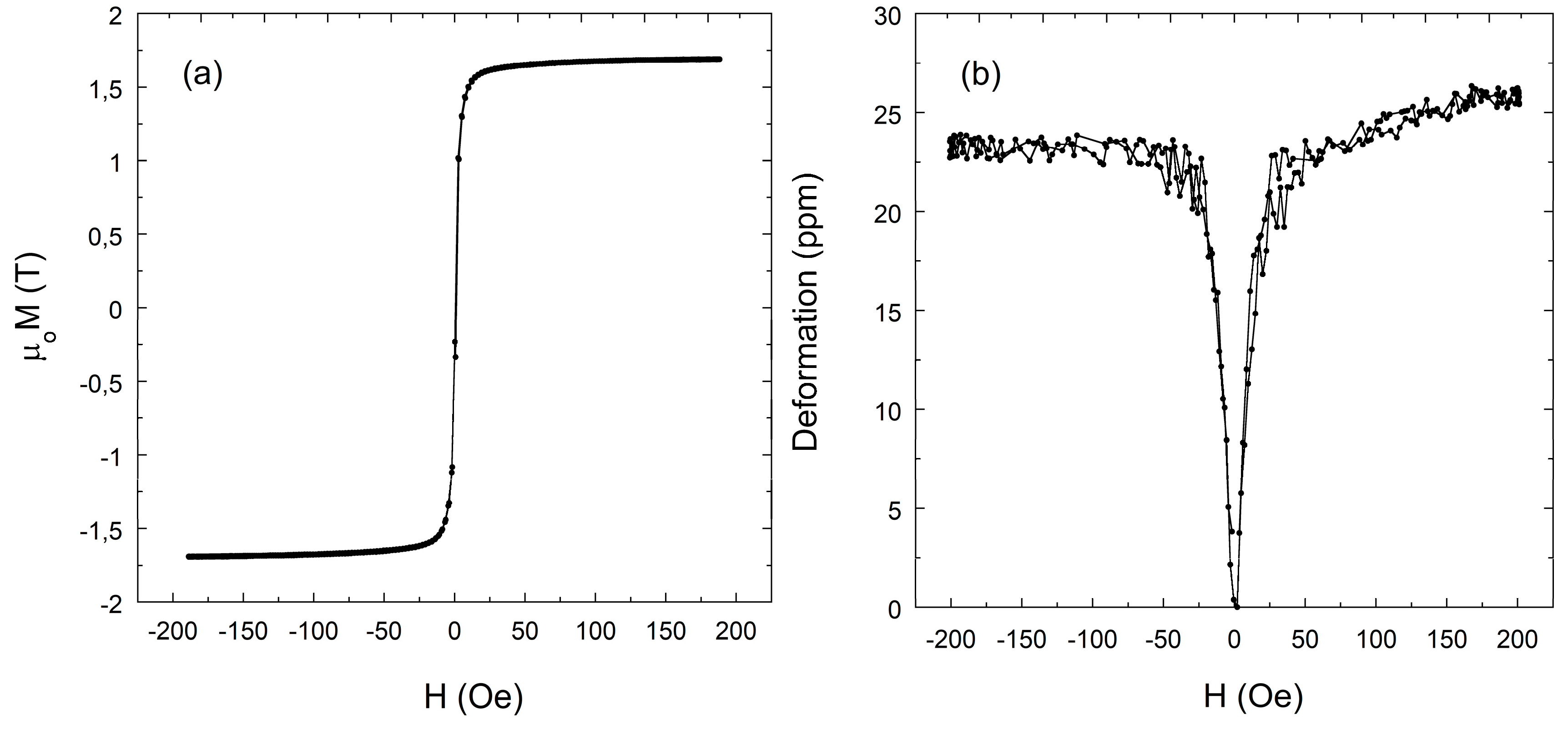
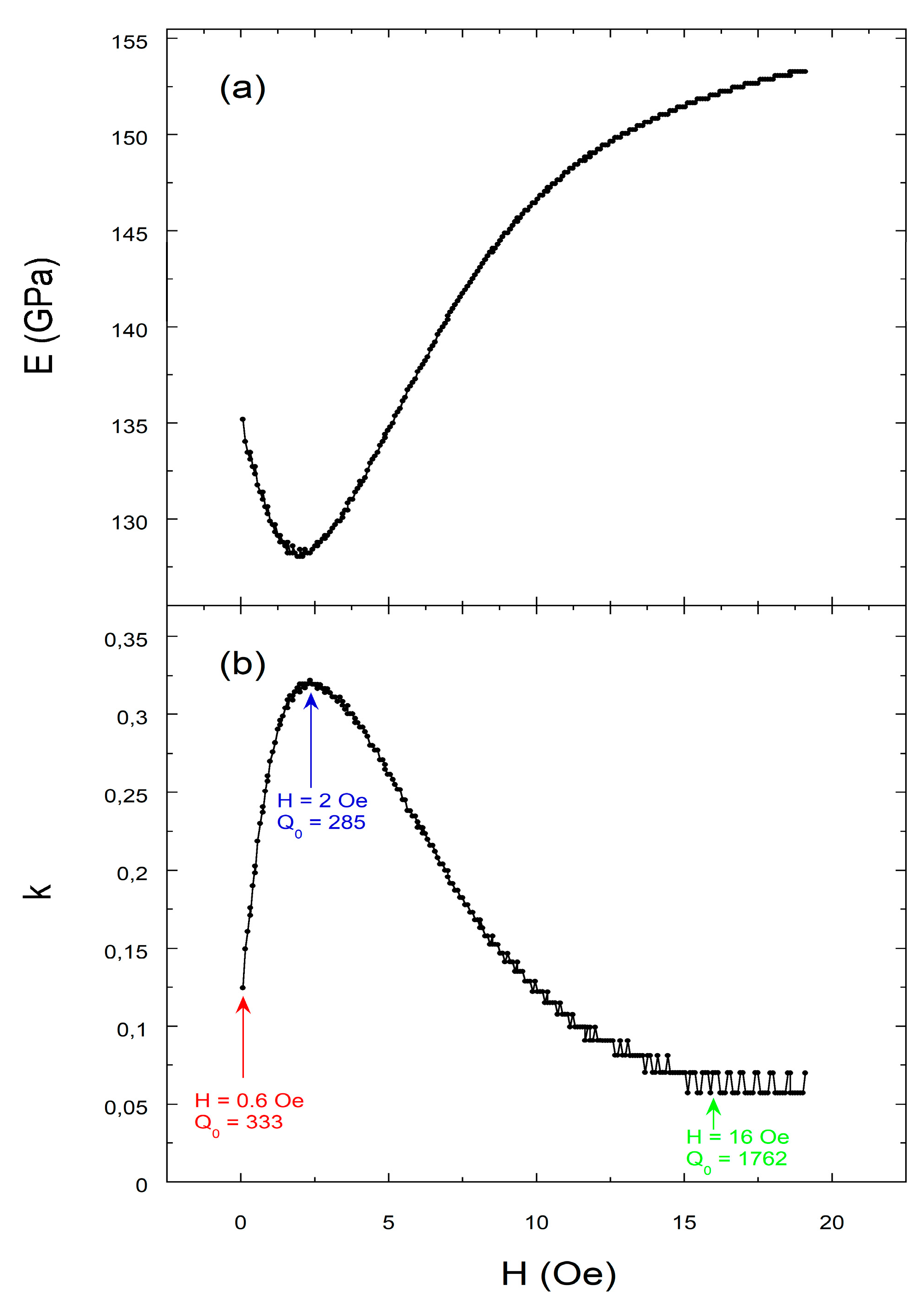
2.1. Material: Magnetic and Magnetostrictive Characterization

In the present study, Fe-based $F{e}_{64}C{o}_{17}S{i}_{6.6}{B}_{12.4}$ composition homemade metallic glass ribbons were used. They were prepared by the single roller quenching method in the form of a long ribbon. Equal length strips ($L=4\mathrm{cm}$) were cut to perform all the magnetic and magnetoelastic characterizations. Room-temperature hysteresis loops were measured by a classical induction method, obtaining a saturation magnetization (given as internal magnetic induction in Tesla) of ${\mu }_o{M}_S\approx 1.6\mathrm{T}$ and a magnetic susceptibility $\chi \approx 15,000$. A magnetostriction value of ${\lambda }_S\approx 22\mathrm{ppm}$ was measured using strain gauges connected to an electronic Wheatstone bridge. Figure 2 shows the obtained hysteresis loop and magnetostriction curves.

2.2. Magnetoelastic Characterization

The metallic glasses of the present study show excellent coupling between magnetic and elastic properties, that is, the applied mechanical stress and the magnetic field generating equivalent effects in the magnetization and deformation of the materials. A direct consequence of the magnetoelastic coupling is the dependence of the elastic constants of magnetostrictive materials on the external magnetic field $H$, in particular the dependence of the longitudinal Young’s modulus on $H$, known as the $\Delta E$ effect ($\Delta E=1-E\left(H\right)/E_S$, with $E_S$ being the Young’s modulus measured at magnetic saturation (a detailed mathematical formula can be found in [21]).

This $\mathsf{\Delta }E$ effect is easy to measure experimentally through the change in mechanical resonance as a function of the field. The resonance can be excited by an alternating field and detected by the changes in magnetic susceptibility. For this purpose, we used a home-mounted, computer-controlled magnetoelastic resonance detection apparatus [22,23] that automatically changes the DC external applied magnetic field $H_{dc}$, also known as bias field, and sweeps the frequency of the AC magnetic field $H_{ac}$ in order to drive the sample to magnetoelastic resonance at a given bias. This is the so-called resonance–antiresonance detection method. We use an HP 3589A Spectrum Analyzer in order to quickly measure the magnitude ($\chi$) of the susceptibility curve at the magnetoelastic resonance and store the resonant frequency $f_r$ at the maximum and antiresonance frequency $f_a$ at the minimum signals, together with the signal amplitude at the resonance. Besides the susceptibility $\chi$, we also measure its real ($\chi \text{'}$) and imaginary ($\chi \text{'}\text{'}$) components separately with the help of a Signal Recovery 7280 Lock-in Amplifier. In these measurements, we extract the frequencies $f{\text{'}}_M$ and $f_m^{\text{'}}$, at the maximum and the minimum signal of the $\chi \text{'}$, respectively, and to the frequency $f\text{'}{\text{'}}_M$ at maximum $\chi \text{'}\text{'}$.

All these measured frequencies and in particular the resonance ($f_r$) vary with the bias field $H_{dc}$, and so does the Young’s modulus, determined as $E\left(H\right)={\left[2L{f}_r^2\left(H\right)\right]}^2\rho$ [24], where $L$ and $\rho$ are the length and density, respectively, of the sample. Other useful magnetoelastic parameters that can be determined from these measurements are the magnetoelastic coupling coefficient ($k=\sqrt{\left({\pi }^2/8\right)\left(1-{\left(f_r/f_a\right)}^2\right)}$) [25] and the quality factor of the resonance $Q$. All such quantities are a function of the applied external magnetic field.

Figure 3 shows the typical external applied magnetic field dependence of Young’s modulus $E\left(H\right)$ and magnetoelastic coupling coefficient $k\left(H\right)$ for our magnetostrictive material. It can be seen that there is a minimum in the $E\left(H\right)$ curve that happens at a value of the applied external magnetic corresponding to $H_k$ or effective anisotropy field of the sample. In the same field, the maximum of $k\left(H\right)$ and minimum of $Q\left(H\right)$ occur. This is an expected behavior since in fact the $k$ value is high when the difference between $f_r$ and $f_a$ is also high, that is, the resonance curve is broad, and so its corresponding $Q$ value (quality of the resonance curve) is poor. While the maximum of the coupling value $k$ guarantees the best sensitivity $S$ of a magnetoelastic resonator working as a biological or chemical sensor [13], the simultaneous occurrence of the worst $Q$ value jeopardizes the accurate determination of the magnetoelastic resonance frequency. Bearing this in mind, we will study the $Q$ factor under external bias field conditions for poor ($k=0.065$ at $16Oe$), medium ($k=0.176$ at $0.6Oe$), and good ($k=0.282$ at $2Oe$) magnetoelastic coupling, aiming to establish the most adequate method (analysis of the real and imaginary part of the susceptibility, numerical fitting of modulus of the susceptibility, and analytical calculations) to determine the quality factor of a magnetoelastic resonance.

3. Results: Determination of the $Q$ Quality Factor Value

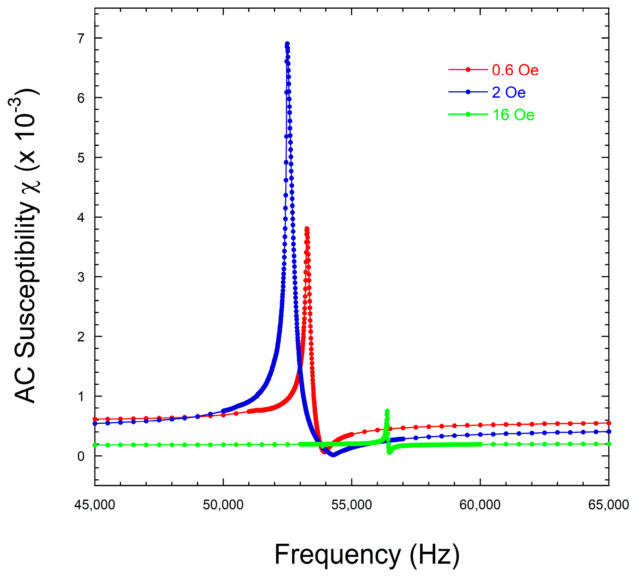
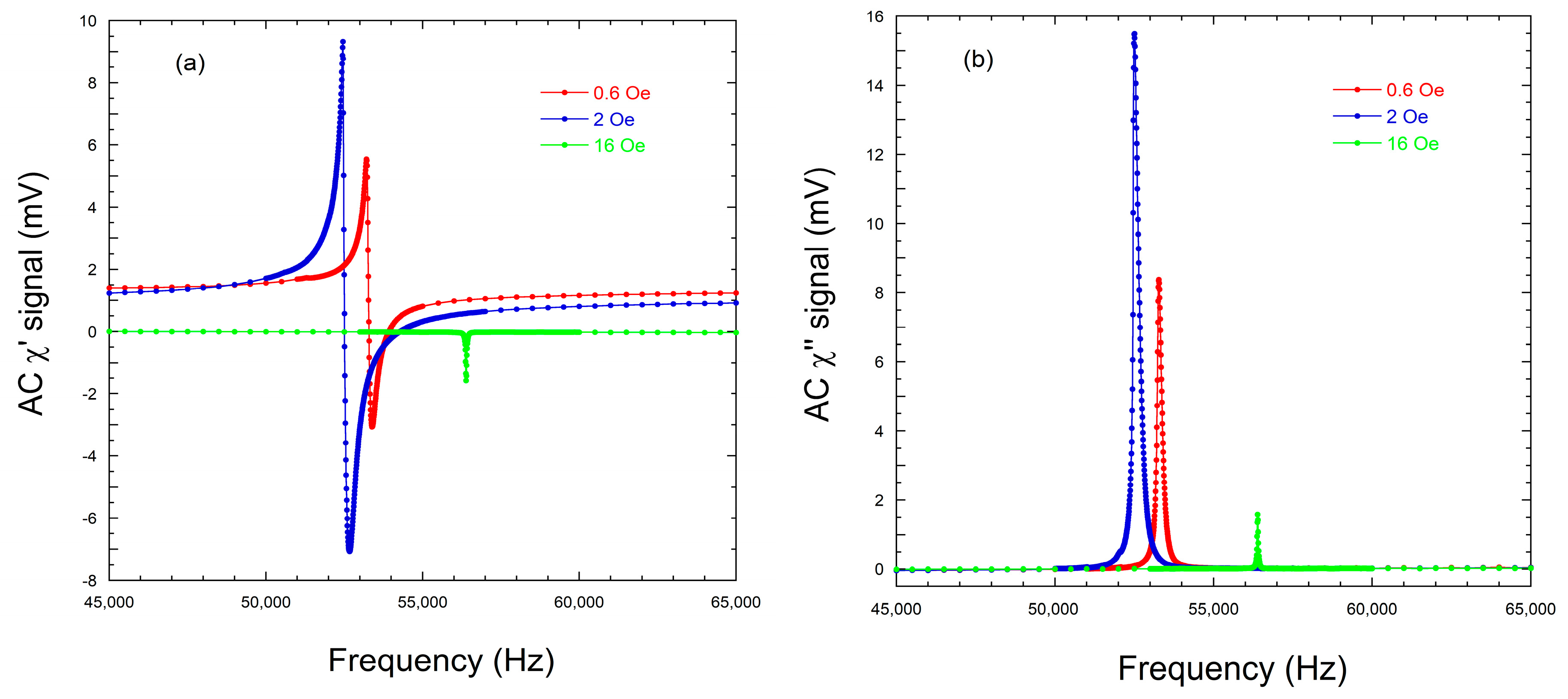
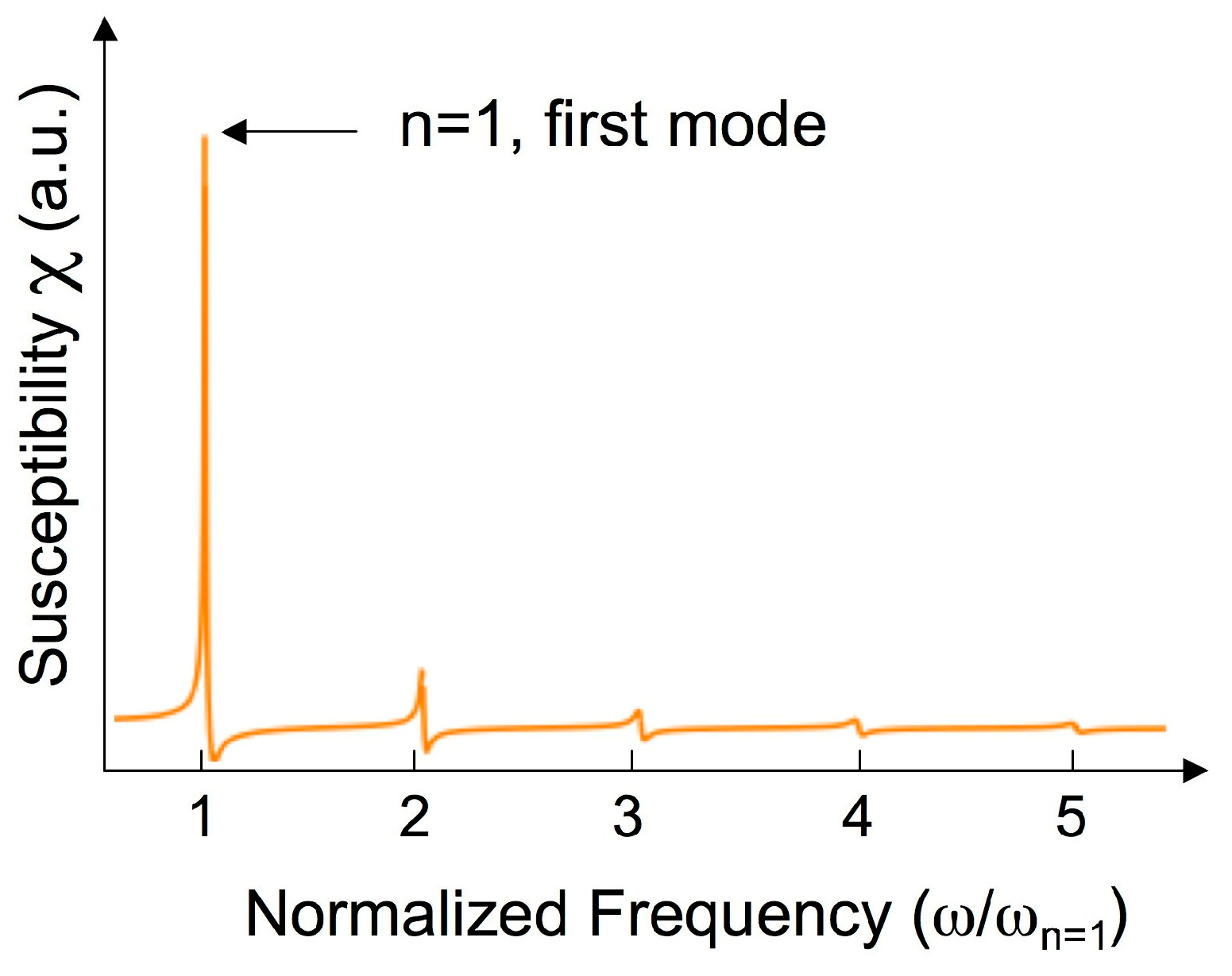
3.1. Full Susceptibility Curve Analysis at Resonance

Figure 4 shows the magnetic susceptibility modulus ($\chi$) curves for our $F{e}_{64}C{o}_{17}S{i}_{6.6}{B}_{12.4}$ ($L=4\mathrm{cm}$) composition metallic glass, measured around the magnetoelastic resonance frequency for all the applied magnetic field cases under study. In these measurements, the frequency step between consecutive points was $10\mathrm{Hz}$.

From these susceptibility modulus ($\chi$) curves, we can directly extract the resonance $(f_r)$ and antiresonance $\left(f_a\right)$ frequencies and so estimate the magnetoelastic coupling coefficient $k$ and the quality factor $Q$, from Equation (2), as

Table 1. Resonance and antiresonance frequencies for $F{e}_{64}C{o}_{17}S{i}_{6.6}{B}_{12.4}$ and calculated k and $Q_0$ values determined directly from the experimental data (this last one obtained using Equation (2)).

$\mathit{H}\left(\mathit{O}\mathit{e}\right)$	${\mathit{f}}_{\mathit{r}}\left(\mathit{H}\mathit{z}\right)$	${\mathit{f}}_{\mathit{a}}\left(\mathit{H}\mathit{z}\right)$	$\mathit{\Delta }\mathit{f}$	$\mathit{k}$	${\mathit{Q}}_0$
$0.6$	$53,260$	$53,940$	$160$	$0.176$	$333$
$2$	$52,496$	$54,280$	$184$	$0.282$	$285$
$16$	$56,380$	$56,476$	$32$	$0.065$	$1762$

summarizes. As mentioned before, however, the values of $Q_0$ are quite inaccurate.

However, a careful measurement of those magnetoelastic resonance curves, using a Lock-in Amplifier, allows us to record the susceptibility real and imaginary parts $({\chi }^{\prime }$ and ${\chi }^{″}$, respectively $)$ as Figure 5 shows.

With the measured frequencies corresponding to maximum and minimum values of $\chi \text{'}$ ($f_M^{\text{'}}$ and $f_m^{\text{'}}$, respectively, see Figure 5a), we can use the first approximated expression often used to give an accurate value of this $Q$ quality factor [20]:

$$Q_1\approx \frac{f_r}{{f^{\prime }}_m-{f^{\prime }}_M}.$$

(3)

Table 2. Frequencies for the maximum and minimum of $\chi \text{'}$ ($f_M^{\text{'}}$ and $f_m^{\text{'}}$, respectively), calculated $Q_1$ values (using Equation (3)) and relative error between $Q_0$ and $Q_1$.

$\mathit{H}\left(\mathit{O}\mathit{e}\right)$	$\mathit{f}{’}_{\mathit{M}}\left(\mathit{H}\mathit{z}\right)$	$\mathit{f}{’}_{\mathit{m}}\left(\mathit{H}\mathit{z}\right)$	${\mathit{Q}}_1$	$\mathbf{Relative}\mathbf{Difference}\left(\mathbf{\%}\right)$ $\left({\mathit{Q}}_0,{\mathit{Q}}_1\right)$
$0.6$	$53,212$	$53,396$	$290$	$13$
$2$	$52,456$	$52,672$	$243$	$15$
$16$	$56,372$	$56,412$	$1410$	$20$

summarizes the experimentally obtained frequency data for maximum and minimum values of $\chi \text{'}$ ($f_M^{\text{'}}$ and $f_m^{\text{'}}$, respectively) and calculated $Q_1$ values from Equation (3), as well as the relative difference between $Q_0$ and $Q_1$.

It must be noted that to separately obtain the real and imaginary parts of the susceptibility is a quite difficult and time-consuming experimental task. Therefore, a method to obtain $Q$ based only on the magnitude or modulus of the susceptibility is highly desirable, though it demands more complex numerical treatment afterwards.

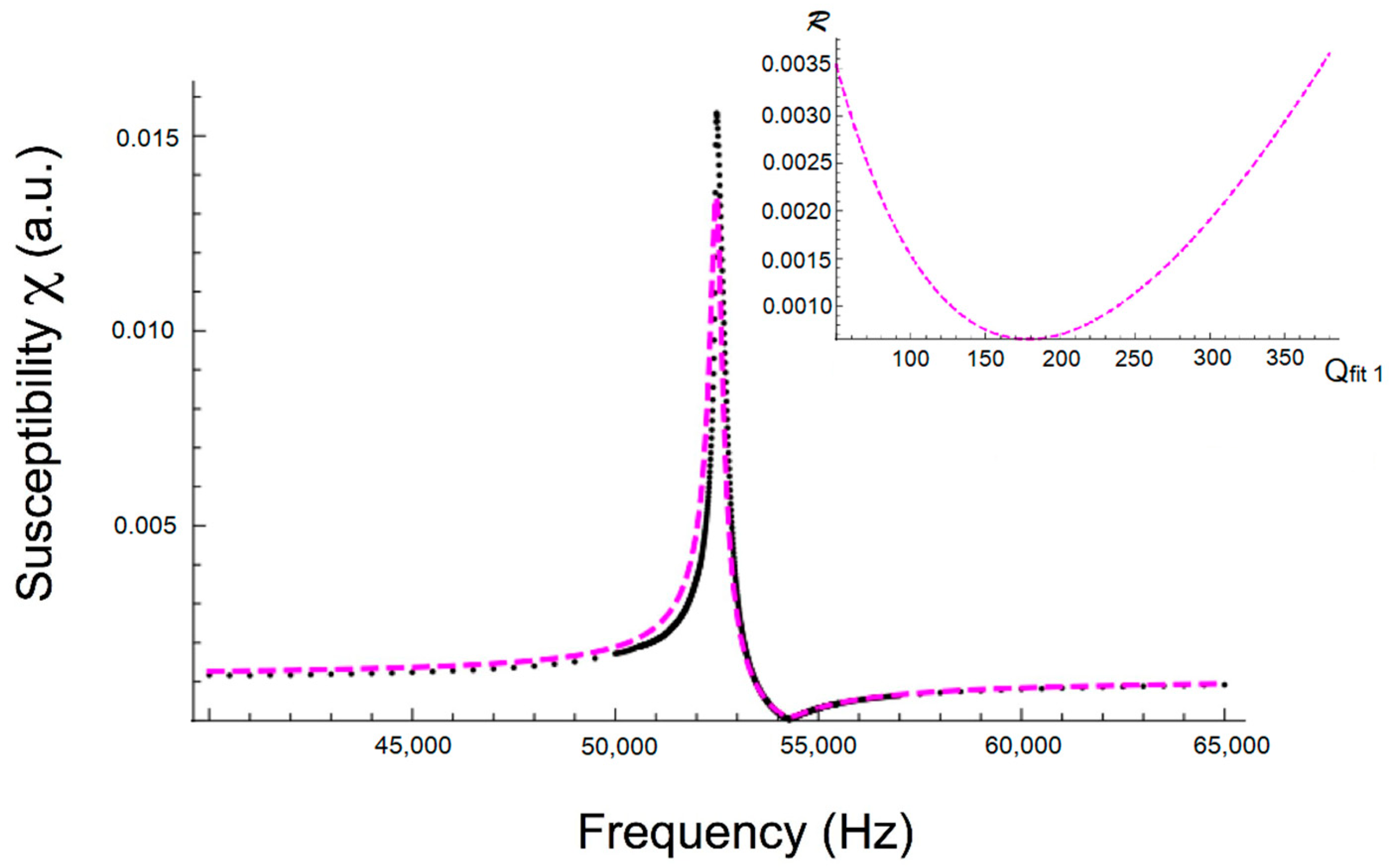
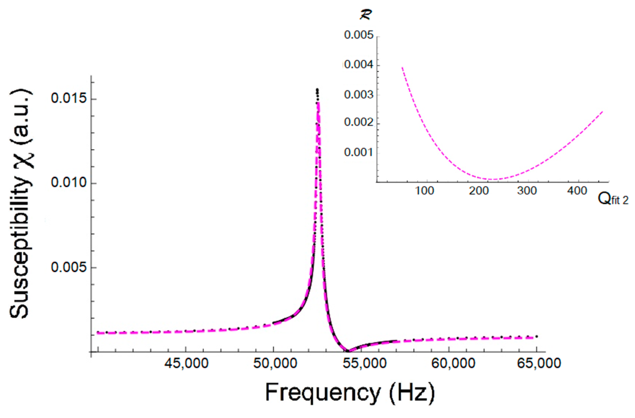
3.2. Numerical Fitting of the Magnitude of the Susceptibility Curve

In 1978 Savage et al. [25] derived the following expression for the susceptibility around the magnetoelastic resonance in a free-standing cylinder-shaped sample:

$$\chi \left(\omega \right)={\chi }_0\left[1-\frac{8k^2}{{\pi }^2}{\displaystyle \sum }_n\frac{1}{n^2}\times \frac{1}{1-\frac{{\omega }_n^2}{{\omega }^2}+i{Q}^{-1}\frac{{\omega }_n}{\omega }}\right],$$

(4)

where $k$ is the magnetoelastic coupling coefficient, ${\omega }_n=2\pi f_n$ is the frequency of the nth harmonic of the excited fundamental mode ($n=1$), $Q^{-1}$ is a phenomenological damping coefficient, and ${\chi }_0$ is the magnetic susceptibility measured at a frequency far below the resonance [26]. Equation (4) also applies to rectangular section ribbons with a proper choice of the $k$ factor. Figure 6 shows an example of the calculated magnetic susceptibility, up to the fifth harmonic, by using Equation (4).

A different approach to estimate $Q$ of a magnetoelastic resonance curve is the numerical fitting of the modulus or magnitude of the experimental susceptibility around its first resonant mode ($n=1$) by using Equation (4). Thus, we proceed to perform numerical fittings using Mathematica© software (v.11.0), following two different strategies: (a) by using the measured $f_r,f_a,{\chi }_0$ values as fixed parameters and (b) by leaving these parameters to vary around the experimentally obtained ones. In both cases, our goal is to search for the optimum $Q$ value that minimizes the $L^2$ norm between the fit and experimental data. We define such a norm (also called residual) as: $ℛ$ $=\frac{1}{N}{\displaystyle \sum }_{i=1,N}{\left(\frac{{\chi }_{exp,i}-{\chi }_{fit,i}}{{\chi }_{max}}\right)}^2$, where ${\chi }_{max}=\max \left({\chi }_{max,exp},{\chi }_{max,fit}\right)$ and $N$ is the number of experimental points. In our measurements, $N=397,691$ and $639$ for $H=0.6,2$ and $16Oe$, respectively. With such a definition, $0\le \mathcal{R}$ $\le 1$, and a value of R close to 0 means very good fitting.

3.2.1. Numerical Fitting of the Susceptibility Curve Using Fixed Parameters

Figure 7 shows the measured magnetoelastic resonance curve at $H=2Oe$ and the fitted one when procedure a) is used. The only free parameter was the quality factor $Q$ with an initial value of $Q_0=285$. The sweep range for $Q$ was $50–380$, and the optimum fitting was found for $Q_{fit1}=178$ (see Figure 7 inset). For all the fits performed, the frequency step between consecutive points will be $1\mathrm{Hz}$. The fit of Figure 7 is the best one obtained by following the a procedure. It looks satisfactory, but can still be improved.

Table 3. $Q$ values from the fitting of the χ susceptibility modulus, using fixed experimental parameters (procedure a).

$\mathit{H}\left(\mathit{O}\mathit{e}\right)$	${\mathit{f}}_{\mathit{r}}\left(\mathit{H}\mathit{z}\right)$	${\mathit{f}}_{\mathit{a}}\left(\mathit{H}\mathit{z}\right)$	${\mathit{Q}}_{\mathit{f}\mathit{i}\mathit{t}1}$	$ℛ$
$0.6$	$53,260$	$53,940$	$208$	$0.0041$
$2$	$52,496$	$54,280$	$178$	$0.0039$
$16$	$56,380$	$56,476$	$1067$	$0.00031$

summarizes the results obtained for the three different magnetic field cases. While all obtained $Q_{fit1}$ values are lower than the previous $Q_0$ ones, it is noticeable that the worst fit corresponds to the applied magnetic field, where magnetoelastic coupling is maximum but quality factor is minimum.

3.2.2. Numerical Fitting of the Susceptibility by Leaving All Parameters Free

Figure 8 shows the measured magnetoelastic resonance curve at $H=2Oe$ and the fitted one when this second procedure is used: all parameters were left free in a range around the starting guess given by the experimental values appearing in Table 1. In this case we swept the $Q$ value in the range $50–440$, finding the best fit for $Q_{fit2}=229$, for the case of applied magnetic field $H=2Oe$ (see Figure 8 inset). Now the fit has greatly improved, as the norm values are much lower, especially for the curve with the highest $Q$ value curve ($atH=16Oe$) (see

Table 4. Obtained parameters (resonance and antiresonance frequencies and $Q$) from the fitting leaving all parameters free (procedure b).

$\mathit{H}\left(\mathit{O}\mathit{e}\right)$	${\mathit{f}}_{\mathit{r}}\left(\mathit{H}\mathit{z}\right)$	${\mathit{f}}_{\mathit{a}}\left(\mathit{H}\mathit{z}\right)$	${\mathit{Q}}_{\mathit{f}\mathit{i}\mathit{t}2}$	$ℛ$
$0.6$	$53,301$	$53,927$	$283$	$0.00027$
$2$	$52,566$	$54,296$	$229$	$0.00060$
$16$	$56,390$	$56,466$	$1321$	$0.000011$

).

Table 4 summarizes the results obtained for the three applied magnetic field cases. Again, as with the first simulation procedure, all obtained $Q_{fit2}$ values are lower than the previous $Q_0$ ones and the worst fit corresponds to the applied magnetic field where magnetoelastic coupling is maximal but the quality factor is minimal.

3.3. An Exact Expression for the $Q$ Factor

Starting with Equation (4) and taking into account the shape of the ${\chi }^{\prime }\left(\omega \right)$ curve, one of us (J.G.) has derive an exact analytical expression for the $Q$ factor value calculation. Since magnetic susceptibility $\chi$ can be described by Equation (4) as a complex number, $\chi =\chi \text{'}+i\chi \text{'}\text{'}$, we can separate the real and imaginary parts of this complex expression (taking into account only the first harmonic, $n=1$) as follows:

$$\frac{\chi \text{'}}{{\chi }_0}=1-\frac{8k^2}{{\pi }^2}\frac{{\omega }^2\left({\omega }^2-{{\omega }_1}^2\right)}{{\left({\omega }^2-{{\omega }_1}^2\right)}^2+{\left(\frac{\omega {\omega }_1}{Q}\right)}^2},$$

(5)

and

$$\frac{\chi \text{'}\text{'}}{{\chi }_0}=\frac{8k^2}{{\pi }^2}\frac{\frac{{\omega }^3{\omega }_1}{Q}}{{\left({\omega }^2-{{\omega }_1}^2\right)}^2+{\left(\frac{\omega {\omega }_1}{Q}\right)}^2}.$$

(6)

The real part shows resonance at its maximum: (${\omega }_M^{\text{'}}$) and antiresonance at its minimum: ($\omega {’}_m$) (see Figure 5a). It is well known that at the local maxima and minima, the derivative vanishes so we can apply this criteria for the frequencies $\omega ={\omega }_M^{\text{'}}$ and $=\omega {‘}_m$:

$$\frac{d}{d\omega }\left(\frac{\chi \text{'}}{{\chi }^{\sigma }}\right)=0=>\frac{d}{d\omega }\frac{{\omega }^2\left({\omega }^2-{{\omega }_1}^2\right)}{{\left({\omega }^2-{{\omega }_1}^2\right)}^2+{\left(\frac{\omega {\omega }_1}{Q}\right)}^2}=0.$$

(7)

After a short calculation, and taking into account that $Q>0$ and single-valued (which means ${\omega }_M<{\omega }_r<{\omega }_m$), the $Q$ factor value can be written in the following two ways:

$$Q=\frac{{{\omega }_m}^2}{{{\omega }_m}^2-{{\omega }_1}^2}\mathrm{and}Q=\frac{{{\omega }_M}^2}{{{\omega }_1}^2-{{\omega }_M}^2}.$$

(8)

Solving these two expressions, first for ${\omega }_M={\omega }_r$ and afterwards for $Q$, we finally get an exact analytical expression for the $Q$ factor value:

$$Q_{cal}=\frac{{\omega }_m^2+{\omega }_M^2}{{\omega }_m^2-{\omega }_M^2}=\frac{1+u^2}{1-u^2},$$

(9)

where $u=\omega {\text{'}}_M/\omega {\text{'}}_m=f{\text{'}}_M/f{\text{'}}_m$.

Table 5. $F{e}_{64}C{o}_{17}S{i}_{6.6}{B}_{12.4}$ experimentally obtained data for resonance and antiresonance frequencies of the real part of the magnetic susceptibility, and calculated $Q$ values using Equation (9).

$\mathit{H}\left(\mathit{O}\mathit{e}\right)$	${\mathit{f}}_{\mathit{M}}^{\text{'}}\left(\mathit{H}\mathit{z}\right)$	${\mathit{f}}_{\mathit{m}}^{\text{'}}\left(\mathit{H}\mathit{z}\right)$	${\mathit{Q}}_{\mathit{c}\mathit{a}\mathit{l}}$
$0.6$	$53,212$	$53,396$	$290$
$2$	$52,456$	$52,672$	$243$
$16$	$56,372$	$56,412$	$1410$

summarizes the experimentally measured values for those frequencies and the subsequently obtained $Q_{cal}$ values.

4. Discussion

All the $Q$ values obtained by the different calculation procedures explained in this study are summarized in

Table 6. $Q$ values for all the applied magnetic field cases, obtained by the different procedures shown in this study.

$\mathit{H}\left(\mathit{O}\mathit{e}\right)$	${\mathit{Q}}_0=\frac{{\mathit{f}}_{\mathit{r}}}{\mathsf{\Delta }\mathit{f}}$	${\mathit{Q}}_1\approx \frac{{\mathit{f}}_{\mathit{r}}}{{\mathit{f}}_{\mathit{m}}^{\text{'}}-{\mathit{f}}_{\mathit{M}}^{\text{'}}}$	${\mathit{Q}}_{\mathit{f}\mathit{i}\mathit{t}1}$	${\mathit{Q}}_{\mathit{f}\mathit{i}\mathit{t}2}$	${\mathit{Q}}_{\mathit{c}\mathit{a}\mathit{l}}=\frac{{\mathit{f}}_{\mathit{m}}^2+{\mathit{f}}_{\mathit{M}}^2}{{\mathit{f}}_{\mathit{m}}^2-{\mathit{f}}_{\mathit{M}}^2}$
$0.6$	$333$	$290$	$208$	$283$	290
$2$	$285$	$243$	$178$	$229$	$243$
$16$	$1762$	$1410$	$1067$	$1321$	$1410$

, while

Table 7. Comparison and estimated errors of the $Q$ values obtained with the different calculation procedures.

$\mathit{H}\left(\mathit{O}\mathit{e}\right)$	$\mathit{E}\mathit{r}\mathit{r}\mathit{o}\mathit{r}\left(\mathbf{\%}\right)\mathit{R}\mathit{e}\mathit{s}\mathit{p}\mathit{e}\mathit{c}\mathit{t}\mathit{t}\mathit{o}{\mathit{Q}}_1\mathit{o}\mathit{r}{\mathit{Q}}_{\mathit{c}\mathit{a}\mathit{l}}$
	${\mathit{Q}}_{\mathit{0}}$	${\mathit{Q}}_{\mathit{f}\mathit{i}\mathit{t}\mathit{1}}$	${\mathit{Q}}_{\mathit{f}\mathit{i}\mathit{t}\mathit{2}}$
$0.6$	$13$	$28$	$2.4$
$2$	$15$	$27$	$5.7$
$16$	$20$	$24$	$6.3$

shows the estimated errors (in %, calculated as $Error\left(\%\right)=\left|\frac{Q_1-Q}{Q_1}\right|·100$) among those obtained $Q$ values. The first thing to notice is that in all cases (or calculation procedures) the higher the estimated $Q$ value, the higher the error in its determination, and this always corresponds to the highest applied field. This is a direct consequence of the sharpness of the measured resonance curves, as well as of its low amplitude (magnetic susceptibility), as can be seen in Figure 5a. As predicted previously by other authors [20], this estimated error (if the classical $Q_0$ definition is used) can be as high as $20\%$. Surprisingly, the obtained norm of the fitting for this high applied field case is the lowest, this is, the numerical fits are the best for this case.

We also found that the values obtained for $Q_1$ (the value given by Kaczkowski [20]) and $Q_{cal}$ (exact analytical expression) are almost equal. While Kaczkowski’s expression was an approximation obtained graphically from the impedance circle of an electrical circuit, our exact formula comes from the analysis of the real part of the magnetic susceptibility around the magnetoelastic resonance.

So, if we only have the possibility of measuring or working with the magnetic susceptibility modulus, numerical fitting of the measured magnetoelastic resonance curve is needed. From the results of the numerical fittings used (as can be observed in Figure 7 and Figure 8 and Table 7), it is clear that the second procedure (leaving all parameters $f_r,f_a$ and ${\chi }_0$ free) leads to a much better result than the first one, as deduced from the obtained lowest norm values for procedure b. That is, we can affirm that the $Q_{fit2}$ value obtained by using fitting procedure b can be considered the best approximation of the true $Q$ quality factor of the magnetoelastic resonance curve.

On the other hand, if we compare the $Q$ values obtained from numerical fits with the approximated $Q_1$ value given by Kaczkowski or with the $Q_{cal}$ value, the estimated error when using fitting procedure a is always higher than $20\%$, while for fitting (procedure b) the range is only approximately $2–6\%$. Thus, $Q_1$ or $Q_{cal}$ can be taken as approximated initial values when performing a numerical fit in order to get the most accurate $Q$ value of a susceptibility magnetoelastic resonance curve.

It is also noticeable that $Q$ values obtained with fitting (procedure b) are systematically lower than $Q_1$ or $Q_{cal}$, but this is a fact that should be expected: Equation (9) gives us the exact quality factor $Q$ of the real part of the magnetic susceptibility around the frequency at which a magnetoelastic resonance happens, with this real part being a sharper curve than the corresponding measured susceptibility modulus. As is already well known, the sharper the curve, the higher the quality factor value. Finally, from the obtained error values, we can affirm that when using a magnetoelastic resonant platform for biological or chemical detection purposes, it is convenient to apply a bias field in the range $0<H_{bias}<H_k$, searching for a compromise between moderate magnetoelastic coupling and low enough error in $Q$ value determination.

5. Conclusions

We have presented an extensive study of the determination of the $Q$ factor of a magnetoelastic resonance curve. This type of resonance is of great interest in order to fabricate devices for biological or chemical detection purposes. The use of the numerical fitting of the magnetic susceptibility modulus around that magnetoelastic resonance turns out to be a useful tool to give accurate $Q$ quality factor values. These differ by up to 20% compared with the $Q$ values determined by following the classical definition. Comparison with approximated $Q$ value given by Kaczkowski and by the exact analytical solution obtained from the real part of the measured susceptibility shows, as expected, that in these two last cases the quality factor value obtained is always slightly higher than that estimated from the numerical fitting. This is a direct consequence of the fact that, while the numerical fit is performed over the magnetic susceptibility modulus, Kaczkowski’s and the exact expression for have been obtained from the real part of that susceptibility curve, which is always sharper than the susceptibility modulus one.

Future work should aim to obtain an analytical expression for the $Q$ quality factor directly obtained from the magnetic susceptibility modulus measured around the magnetoelastic resonance.

References

- Grimes, C.A.; Seitz, W.R.; Horn, J.; Doherty, S.A.; Rooney, M.T. A remotely interrogatable magnetochemical pH sensor. IEEE Trans. Magn. 1997, 33, 3412–3414. [Google Scholar] [CrossRef]
- Stoyanov, P.G.; Doherty, S.A.; Grimes, C.A.; Seitz, W.R. A remotely interrogatable sensor for chemical monitoring. IEEE Trans. Magn. 1998, 34, 1315–1317. [Google Scholar] [CrossRef] [PubMed]
- Grimes, C.A.; Mungle, C.S.; Zeng, K.; Jain, M.K.; Dreschel, W.R.; Paulose, M.; Ong, G.K. Wireless magnetoelastic resonance sensors: A critical review. Sensors 2002, 2, 294–313. [Google Scholar] [CrossRef]
- Bouropoulos, N.; Kouzoudis, D.; Grimes, C.A. The real-time, in situ monitoring of calcium oxalate and brushite precipitation using magnetoelastic sensors. Sens. Actuators B 2005, 109, 227–232. [Google Scholar] [CrossRef]
- Grimes, C.A.; Kouzoudis, D.; Dickey, E.C.; Kiang, D.; Anderson, M.A.; Shahidain, R.; Lindsey, M.; Green, L. Magnetoelastic sensors in combination with nanometer-scale honeycombed thin film ceramic TiO2 for remote query measurement of humidity. J. Appl. Phys. 2000, 87, 5341–5343. [Google Scholar] [CrossRef] [PubMed]
- Cai, Q.Y.; Cammers-Goodwin, A.; Grimes, C.A. A wireless, remote query magnetoelastic CO2 sensor. J. Environ. Monit. 2000, 2, 556–560. [Google Scholar] [CrossRef] [PubMed]
- Baimpos, T.; Gora, L.; Nikolakis, V.; Kouzoudis, D. Selective detection of hazardous VOCs using zeolite/Metglas composite sensors. Sens. Actuators A 2012, 186, 21–31. [Google Scholar] [CrossRef]
- Lakshmanan, R.S.; Guntupalli, R.; Hu, J.; Kim, D.J.; Petrenko, V.A.; Barbaree, J.M.; Chin, B.A. Phage immobilized magnetoelastic sensor for the detection of Salmonella typhimurium. J. Microbiol. Methods 2007, 71, 55–60. [Google Scholar] [CrossRef] [PubMed]
- Huang, S.; Yang, H.; Lakshmanan, R.S.; Johnson, M.L.; Wan, J.; Chen, I.H.; Wikle, H.C., III; Petrenko, V.A.; Barbaree, J.M.; Chin, B.A. Sequential detection of Salmonella typhimurium and Bacillus anthracis spores using magnetoelastic biosensors. Biosens. Bioelectron. 2009, 24, 1730–1736. [Google Scholar] [CrossRef] [PubMed]
- Ruan, C.; Zeng, K.; Varghese, O.K.; Grimes, C.A. Magnetoelastic immunosensors: Amplified mass immunosorbent assay for detection of Escherichia coli O157:H7. Anal. Chem. 2003, 75, 6494–6498. [Google Scholar] [CrossRef] [PubMed]
- Luborsky, F.E. Chapter 6: Amorphous ferromagnets in Ferromagnetic Materials. In Handbook of Ferromagnetic Materials; Wohlfart, E.P., Ed.; Elsevier: Amsterdam, The Netherlands, 1980; Volume 1, ISBN 0-444-85311-1. [Google Scholar]
- Stoyanov, P.G.; Grimes, C.A. A remote query magnetostrictive viscosity sensor. Sens. Actuators A 2000, 80, 8–14. [Google Scholar] [CrossRef]
- Sagasti, A.; Gutiérrez, J.; Sebastián, M.S.; Barandiarán, J.M. Magnetoelastic resonators for highly specific chemical and biological detection: A critical study. IEEE Trans. Magn. 2017, 53, 4000604. [Google Scholar] [CrossRef]
- Sagasti, A. Functionalized Magnetoelastic Resonant Platforms for Chemical and Biological Detection Purposes. Ph.D. Thesis, University of the Basque Country (UPV/EHU), Leioa, Spain, 2018, unpublished. [Google Scholar]
- Grimes, C.A.; Kouzoudis, D.; Ong, K.G.; Crump, R. Thin-film magnetoelastic microsensors for remote query biomedical monitoring. Biomed. Microdevices 1999, 2, 51–60. [Google Scholar] [CrossRef]
- Bravo-Ímaz, I.; García-Arribas, A.; Gorritxategi, E.; Arnaiz, A.; Barandiarán, J.M. Magnetoelastic viscosity sensor for on-line status assessment of lubricant oils. IEEE Trans. Magn. 2013, 49, 113–116. [Google Scholar] [CrossRef]
- Sagasti, A.; Bouropoulos, N.; Kouzoudis, D.; Panagiotopoulos, A.; Topoglidis, E.; Gutierrez, J. Nanostructured ZnO in Metglas/ZnO/Hemoglobin modified electrode to detect the oxidation of the hemoglobin simultaneously by cyclic voltammetry and magnetoelastic resonance. Materials 2017, 10, 849. [Google Scholar] [CrossRef] [PubMed]
- Peterson, P.J.; Anlage, S.M. Measurement of resonant frequency and quality factor of microwave resonators: Comparison of methods. J. Appl. Phys. 1998, 84, 3392–3402. [Google Scholar] [CrossRef]
- Cory, D.; Hutchinson, I.; Chaniotakis, M. Introduction to Electronics, Signals and Measurements; Springer: Berlin, Germany, 2006; Chapter 17. [Google Scholar]
- Kaczkowski, Z. Piezomagnetic dynamics as a new parameter of magnetostrictive materials and transducers. Bull. Pol. Acad. Sci. 1997, 45, 19–42. [Google Scholar]
- Du Tremolet de Laichesserie, E. Magnetostriction: Theory and Application of Magnetoelasticity; CRC Press: Boca Raton, FL, USA, 1993; ISBN 0849369347. [Google Scholar]
- Gutiérrez, J.; Barandiarán, J.M.; Nielsen, O.V. Magnetoelastic properties of some Fe-rich Fe-Co-Si-B metallic glasses. Phys. Status Solidi A 1989, 111, 279–283. [Google Scholar] [CrossRef]
- Gutiérrez, J. Propiedades Magnéticas y Magnetoelásticas de Nuevas Aleaciones Amorfas de Interés Tecnológico. Ph.D. Thesis, University of the Basque Country (UPV/EHU), Leioa, Spain, 1992. [Google Scholar]
- Landau, L.D.; Lifshitz, E.M. Theory of Elasticity; Oxford Pergamon Press: Oxford, UK, 1975; p. 116. [Google Scholar]
- Savage, H.; Abbundi, R. Perpendicular susceptibility, magnetomechanical coupling and shear modulus in Tb0.27Dy0.73Fe2. IEEE Trans. Magn. 1978, 14, 545–547. [Google Scholar] [CrossRef]
- Hernando, A.; Madurga, V.; Barandiarán, J.M.; Liniers, M. Anomalous eddy currents in magnetostrictive amorphous ferromagnets: A large contribution from magnetoelastic effects. J. Magn. Magn. Mater. 1982, 28, 109–116. [Google Scholar] [CrossRef]