Holey-Cavity-Based Compressive Sensing for Ultrasound Imaging
by
 ,
,
Ashkan Ghanbarzadeh-Dagheyan
1 ,
,
Chang Liu
1,
Ali Molaei
2,
Juan Heredia
1,2 and
Jose Martinez Lorenzo
1,2,* 1
Mechanical Engineering Department, Northeastern University, Boston, MA 02115, USA
2
Electrical Engineering Department, Northeastern University, Boston, MA 02115, USA
*
Author to whom correspondence should be addressed.
Sensors 2018, 18(6), 1674; https://doi.org/10.3390/s18061674
Submission received: 25 January 2018
/
Revised: 9 April 2018
/
Accepted: 19 April 2018
/
Published: 23 May 2018
(This article belongs to the Special Issue Ultrasonic Sensors 2018)
Abstract
:The use of solid cavities around electromagnetic sources has been recently reported as a mechanism to provide enhanced images at microwave frequencies. These cavities are used as measurement randomizers; and they compress the wave fields at the physical layer. As a result of this compression, the amount of information collected by the sensing array through the different excited modes inside the resonant cavity is increased when compared to that obtained by no-cavity approaches. In this work, a two-dimensional cavity, having multiple openings, is used to perform such a compression for ultrasound imaging. Moreover, compressive sensing techniques are used for sparse signal retrieval with a limited number of operating transceivers. As a proof-of-concept of this theoretical investigation, two point-like targets located in a uniform background medium are imaged in the presence and the absence of the cavity. In addition, an analysis of the sensing capacity and the shape of the point spread function is also carried out for the aforementioned cases. The cavity is designed to have the maximum sensing capacity given different materials and opening sizes. It is demonstrated that the use of a cavity, whether it is made of plastic or metal, can significantly enhance the sensing capacity and the point spread function of a focused beam. The imaging performance is also improved in terms cross-range resolution when compared to the no-cavity case.
1. Introduction
According to Compressive Sensing (CS) theory, unknown signals sampled at a rate smaller than that required by the Shannon–Nyquist theorem [1] may be recovered when certain conditions are satisfied. Specifically, the CS theory relies on two mathematical principles: sparsity, which imposes that the unknown signal must accept a sparse representation in a known dictionary or set of base functions; and incoherence, which requires that the Restricted Isometry Property (RIP) is satisfied by the sensing matrix that linearly relates the coefficients of the unknown signal and the undersampled data [2,3]. It can be shown that the smaller the coherence between each of two columns of the sensing matrix, the more accurately the unknown signal can be recovered [3]. When the sensing matrix is built through random projections in the undersampled signal space, the resulting coherence between each of two of its columns is small, with a high probability. This is the reason why measurement randomization has the potential to enhance the accuracy of the recovered unknown signal [2].
Several sensing and imaging applications [4] have been able to take advantage of CS by using pseudo-random illumination in the outgoing waves from the transmitters and collecting pseudo-random measurements from the incoming waves to the receivers. Carin et al. used random positions for the elements of a sensing array to make use of CS. They also showed that placing spherical scattering objects in front of the waves increases the randomness and incoherence of the measurements [5]. Incoherence between each of two measurements can also be achieved by using physical structures that exhibit different wave-matter responses at different instantaneous frequencies, without the need to change the arrangement of the sensing array. For instance, Fromenteze et al. used a metal cavity with a number of holes and a wave agitator inside the cavity to randomize the electromagnetic wave patterns for microwave imaging [6]. Later, the same research group fabricated a metalized cavity with holes arranged in irises following Fibonacci patterns to code the outgoing waves based on frequency diversity [7].
Metamaterials have also been used to create randomness in the sensing system for applications such as microwave imaging [8,9,10], optical imaging [11,12], milliliter-wave imaging [13,14,15,16] and acoustic multichannel separation using a single sensor [17]. The fabrication of holey cavities is generally simpler than that of metamaterials, and they do not require any alteration in the sensing array assortment in contrast to the approach adopted in [5]. Other methods of wave randomization have been proposed in the literature. Specifically for ultrasound imaging, Schiffner introduced a software-based technique that uses time delays and apodization weights to generate random incident acoustic fields [18,19]. Other software methods, which usually involve novel sampling methods, have been proposed, as well [20,21]. Similar to coded masks that are commonly used in compressive optical imaging [22,23,24] as a subgroup of hardware-based methods, Kruizinga et al. introduced a rotating mask of randomly-varying thicknesses throughout its surface to randomize ultrasound waves, and they were able to retrieve 3D images of objects using a single transducer [25]. In this study, a static 2D cavity has been selected as a structure that enables randomization of the wave fields in three generalized dimensions, one spectral and two spatial, thus leading to enhanced ultrasound imaging via compressive sensing. Other types of ultrasound cavities have also been proposed by Fink et al. to create images using time-reversal techniques [26,27,28,29]. However, they have not been used in the scope of compressive sensing; and therefore, their method requires a large number of measurements [25]. In the succeeding sections, the performance of several 2D holey cavities are studied, showing how the cavity-based imaging performance is enhanced when compared to that of a traditional ultrasound imaging setup.
2. Two-Dimensional Cavity
In order to design the cavity, a baseline configuration is defined as shown in Figure 1. It includes a coupling liquid region that contains the ultrasound sources, an interface region and an imaging region that contains the unknown targets surrounded by a known homogeneous background. In many applications, the ultrasound probe is not in direct contact with the imaging domain; therefore, the interface medium was introduced to take into consideration this fact. One example of a 2D cavity enclosing the exciting sources is shown in the top layer of Figure 1. As observed, the cavity is closed from all sides except the bottom, where a number of openings is made for the impinging waves to pass through. It is assumed that the openings are uniformly distributed along the bottom of the cavity, and they are symmetric with respect to the y axis.
3. Compressive Sensing, Imaging and Performance Metrics
In this section, the algorithms used to perform compressive sensing and imaging are introduced. Specifically, a computational forward model is used to simulate the sensing process and measured acoustic wave fields, the inverse model is formulated and the first-order Born approximation is used as a simple approach to linearize the imaging problem. Moreover, the sensing capacity and the Point Spread Function (PSF) of the system are defined, and they will be used as extra metrics to assess how the addition of the cavity affects the performance of the imaging system.
3.1. The Forward Model
For an inhomogeneous medium, with its density and speed of sound defined as a function of the location vector , the linear wave equation for a time-harmonic pressure field can be expressed as follows [30]:
in which is the angular frequency with f denoting the frequency, is the density, is the wavenumber, is the pressure field and is the acoustic source term, all defined in the medium. The mathematical model of depends on how the source is defined. If the exciting source is a monopole, and it is defined based on the Root Mean Square (RMS) of power per unit length, i.e., , then [31]
where and are the phase and the location of the source, respectively, and is the Dirac delta function, shifted from the origin to the source location. To excite a delta function having a magnitude of one (pascals per unit area) and no phase terms, the parameters must be chosen as and . Equation (1) is solved for the complete geometry shown in Figure 1 using the finite-element software COMSOL Multiphysics (CM), one time with the targets present and one time when they are absent. The former case gives the background field, and the later one gives the total field, both of which will be used in the inverse model to retrieve the image of the targets, as will be discussed in the succeeding subsection. The outer boundaries of the entire simulation domain on all sides are set to be absorbing. Moreover, since the Pressure Acoustics Module of CM is used, the cavity and other solids in the medium are viewed as fluids by the module in terms of wave propagation. In this way, each material in the simulation domain is characterized by its density and longitudinal speed of sound. This method offers an approximation of solid behavior without the need to use the Solid Mechanics Module, and it has been previously used in the literature [32].
3.2. The Inverse Model
The computed total and background fields in the forward modeling inside the imaging domain can be denoted with and . When the targets are small and the density gradient between the targets and the homogeneous background medium is relatively small, and both satisfy the homogeneous and approximated version of Equation (1):
which are in the form of the linear, homogeneous Helmholtz equations. Here, and denote the wavenumbers in the absence and presence of the targets, respectively. If the scattered field is defined as , then Equation (3) can be rewritten as:
Next, subtracting Equation (5) from Equation (4), one can easily show that:
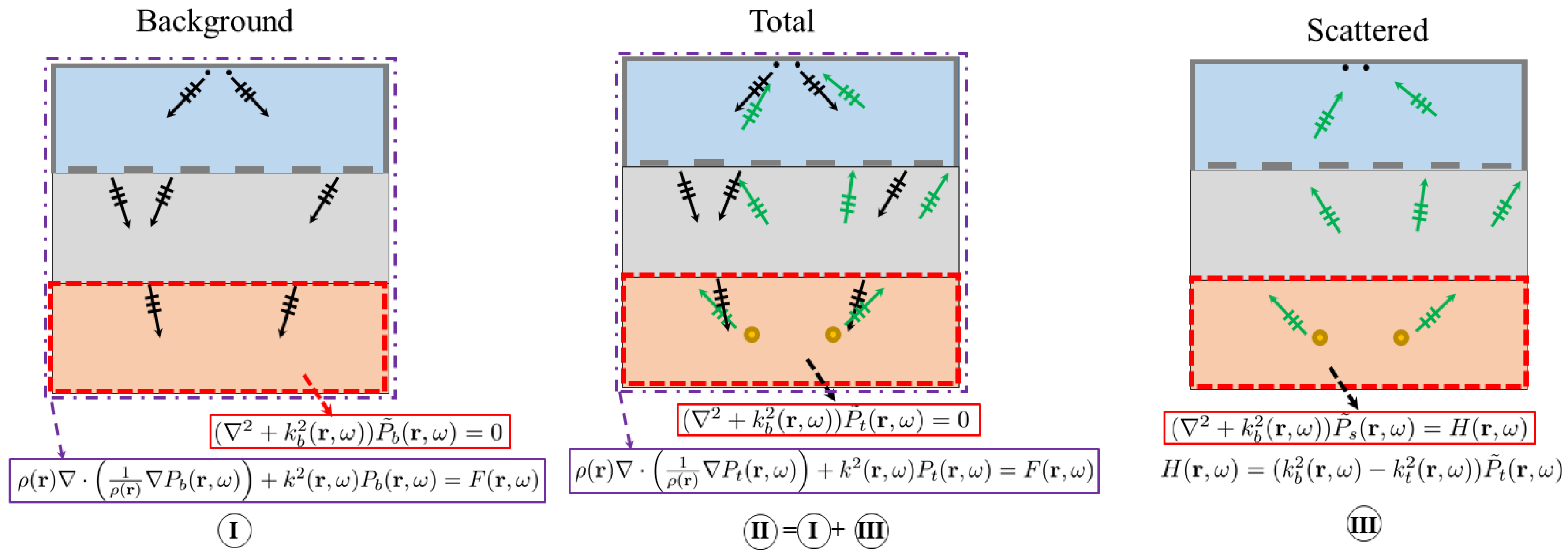
which is similar to (3) and (4), except the exciting source and the subscript s, which stands for the scattered field. The application of the Helmholtz equation in the background, total and scattered field is summarized in Figure 2. The solution to Equation (6) can be obtained by superposition as [33]:
in which is the solution of the background pressure when the exciting source is an impulse function at location ; is the contrast variable and the relationships and are used with and being the speed of sound inside the domain in the presence and the absence of targets, respectively. The subscript denotes the area on which the integrand is integrated, which is the imaging domain. It should be noted that inside the imaging domain, is zero everywhere, save the inside and on the boundaries of the targets. Green’s function is also calculated numerically using a full-field simulation for each frequency and for the entire simulation domain, including the cavity, but without the targets.
The introduced parameter is to be solved for in the imaging problem as the unknown. Provided that the speed of sound does not vary much in the frequency band used [34], the dependence of the contrast variable on frequency may be neglected, i.e., . When the contrast variable is relatively small, causing a small perturbation in the fields, the total field can be estimated from the background field using the first-order Born approximation [35,36], which turns Equation (7) into:
where is to be numerically computed and is obtained by subtracting the simulated total field and background field at the position of the receivers.
3.3. Distributed Compressive Sensing and Imaging Algorithm
Discretizing Equation (8) into P pixels in the imaging domain and having M noiseless measurements on the receivers leads to the following matrix-form equation:
in which is the measurement vector, is the sensing matrix and is the estimated unknown vector—the column-wise stacking of the values of the contrast parameter at each pixel in the imaging domain that will be later reshaped into the actual size of the that domain to give the 2D image. The number of pixels P is determined by the mesh grid in which the fields are exported; and it equals , where and are the size of the grid in the x and y direction, respectively (Figure 1). If the number of transmitters, receivers and the frequencies used in the measurements are respectively denoted by , and , the number of measurements equals , which is explained in details in the Appendix. The system of equations in (9) is underdetermined, since the number of measurements M is usually much smaller than the number of unknowns P. Therefore, an optimization method is needed to find an optimal solution for the system out of infinitely many solutions, particularly in this case where compressed sensing is considered. A norm-one optimization technique called the Alternating Direction Method of Multipliers (ADMM) is employed to find an optimized solution for in a fully-distributed fashion. The version of the ADMM used in this study makes use of parallel computing [37] in Q levels, and it is formulated as follows [38,39]:
in which matrix has been segmented based on rows into Q submatrices , is the solution provided by the submatrix , is the subvector of that is associated with , is the norm-one regularization parameter and is the consensus solution obtained after combining all solutions . The Lagrangian form of Equation (10) is as follows [37] (§3.1):
where is the augmented Lagrangian parameter and is the scaled form of the Lagrangian multiplier [37] (§3.1.1). This problem can be optimized iteratively as presented in Algorithm 1.
| Algorithm 1 Consensus ADMM. | |
| Inputs: | |
| sensing matrix | |
| measurement vector | |
| ← maximum number of iterations | |
| number of rows divisions | |
| augmented Lagrangian parameter | |
| norm-one regularization parameter | |
| Initialize | ▹ Initialization |
| Compute the inverse factor for | |
| iteration number | |
| repeat | |
| for | ▹ Update |
| ▹ Mean of | |
| ▹ Mean of | |
| ▹ Update | |
| for | ▹ Update |
| ▹ Increment k | |
| until | ▹ Check for convergence |
| Output: | |
In the algorithm, denotes the identity matrix, and are, respectively, the mean values of and for all i and is the soft thresholding operator, which is applied on each element of the vector. When it applies on a scalar , it functions as [39,40]:
To calculate the inversion of , where denotes the Hermitian of the sensing matrix, more efficiently, the matrix inversion lemma can be used, as described in [38].
When there is noise in the measurements, Equation (9) can be rewritten as:
where is the noise column vector, having the same size as , is the measurement vector including noise and is signal retrieved from noisy measurements. The imaging results using both noiseless measurements and measurement including noise will be presented in the Section 4.
3.4. Beam Focusing
The performance of the sensing array with and without the cavity can be seen through its PSF, which is the field distribution that results from coherently adding up the pressure field of each transmitter (or receiver), multiplied by a phase term that produces a constructive interference at the focusing point, when the transmitter (or receiver) is excited by a unit impulse function. The described procedure is named phase-based beam focusing, and the resulting PSF for transmitters is given by the following equation [13,41]:
in which is the background field due to transmitter i at location at frequency and is the phase of the background field at the location of the focus point , i.e., .
3.5. Sensing Capacity
Another metric that will be used to assess the performance of the imaging system is the so-called sensing capacity. This metric determines the amount of information that can be transferred from the imaging domain into the sensors; and the larger the sensing capacity is, the better the image reconstruction will be. The sensing capacity, expressed in bits/s/Hz, is computed as follows [41,42]:
where r is the Signal-to-Noise Ratio (), is the i-th nonzero singular value of the sensing matrix—when the values are arranged in ascending order, and q is the number of active transceivers. As observed, C is closely related to the singular values of the sensing matrix, which itself is contingent upon the sensing array and how it has been configured.
4. Simulation Results and Discussion
The goal of this section is to compare the performance of the imaging system with and without the cavity. Specifically, the performance will be assessed in terms of the sensing capacity, the PSF of a focused beam and the image quality. A typical ultrasound imaging medium, which satisfies both the density and contrast conditions, is used as a case study in this paper according to the geometry shown in Figure 1; see Table 1 and the references therein for material properties. As shown in Figure 1, a small number of transceivers (only two) are considered here to show the general concept and the imaging capability using compressive sensing. What is more, two point-like targets are selected to be imaged. Based on the values in Table 1, one can observe that: (i) the contrast variable takes a relatively small value (about 7.84%) at the location of the targets, and it is equal to zero in the background medium; (ii) the targets are comparatively small compared; and (iii) the density difference between the targets and the background medium is about 4%. Thus, the approximations made to obtain Equation (8) can be assumed to be valid and it will be shown that this is indeed the case in the imaging results.
To export the fields, the simulation domain is discretized into a mesh grid size of . The imaging domain has a grid size of and in the x and y direction, in order, leading to a vector signal size of elements. The frequency band is 2–10 MHz, and the frequency steps in the sweeping are 0.1 MHz. The number of transmitters , receivers , and frequencies used in the simulations is 2, 2 and 81, which yields a total measurement number of . It is lucid that these values for M and P make the system in (9) underdetermined since .
4.1. The Effect of the Cavity Design on Sensing Capacity
As introduced in Section 2, there are a number of parameters that can be adjusted in the cavity design. Thus, before any imaging or beam focusing is performed, the cavity parameters are required to be selected. In this study, maximizing the sensing capacity was selected as the design goal, and two parameters of the cavity were adjusted to achieve this end: the opening size and the material of the cavity. The numeric values of the geometric parameters used in the simulations, except and , which are variable in the cavity design, are given in Table 2.
4.1.1. The Size of the Openings
To have the ability to sample all the cavity modes, the size of the openings in the cavity needs to be smaller than the minimum guided wavelength [6]. The frequency band for the simulations in this study is selected to be 2–10 MHz, which covers the typical frequencies used in high resolution ultrasound devices [52]. Hence, the opening size is limited by the lowest wavelength in water corresponding to the highest frequency, that is mm, with being in and in . On the other hand, the hardships in fabrication and micromachining set a limit on how small the openings can be.
Eight different cases are studied, in which the cavity thickness and its material (steel) are kept constant as the size of the holes at the bottom of the cavity was changed. The number of holes is maximized in each case by fitting as many openings as possible at the bottom of the cavity, with the assumption that . Moreover, the openings are generated symmetrically with respect to the y axis, as mentioned before. The results of the sensing capacity versus are shown in Figure 3. It is evident that the addition of the cavity to the simulation domain has increased the sensing capacity; however, the alterations in the opening sizes have not made a significant difference, at least in the units used in the plots. With this setup, the largest opening size () has resulted in the largest sensing capacity among other opening sizes, and at the same time, it is the easiest to fabricate in terms of feature size.
4.1.2. Material Selection
3D printing technology has made prototype fabrication much easier for many applications [53,54,55]. Hence, it is of interest to inspect whether using a 3D printing material such as VeroWhitePlus, which is not as stiff and dense as steel, can adequately randomize the wave fields for compressive sensing. Furthermore, another material, aluminum, is tested as the cavity material, and its effect on the sensing capacity is studied, alongside with that of steel. The results, in terms of sensing capacity difference with the no-cavity case, are illustrated in Figure 4. The sensing capacity difference is defined as below:
in which and are the sensing capacity values obtained by (15) in the presence and absence of the cavity, respectively.
Although the addition of the plastic cavity to the domain has increased the sensing capacity, its effect is not as strong as that of the steel or the aluminum cavity. Since aluminum is lighter than steel, it can be made into thin layers, and its effect in the cavity is close to that of steel, so it was selected as the material for the cavity. It is noteworthy to remark that the maximum capacity difference occurs when the is about 40 dB. Figure 5 shows the wave pattern randomization at four different frequencies in the 2–10-MHz interval for the aluminum-cavity case. It is easy to observe that the field patterns have a reduced correlation as a result of pseudo-random illumination of the scene.
4.2. The Effect of the Cavity on Imaging and Point Spread Function
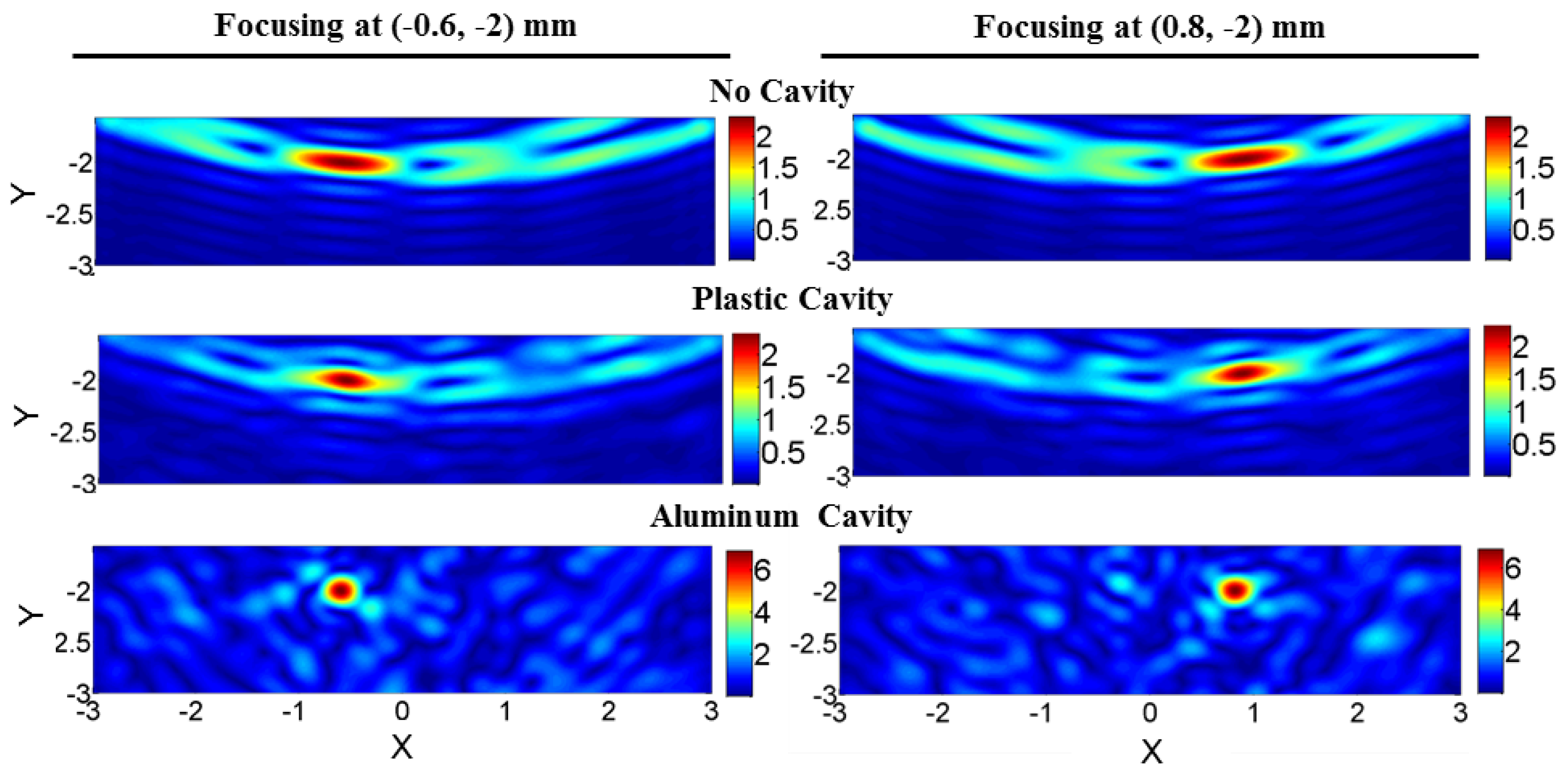
The cavity effect on the PSF of a focused beam is shown for three cases in Figure 6: (i) without the cavity, (ii) when a plastic cavity encloses the sources and (iii) when an aluminum cavity encloses the sources. The PSF of the imaging system improves considerably when the aluminum cavity was used. Specifically, the cross-range aliasing effects are eliminated, and the cross-range resolution is enhanced; nevertheless, this enhancement is not as significant when the plastic cavity is employed.
Figure 7 illustrates the images created from noiseless measurements for the same three cases, alongside the ADMM input parameter values for each case. The maximum number of iterations is selected such that the convergence is ensured, and the number of row divisions Q is selected such that a relatively quick consensus-based solution is achieved. Selecting Q to be relatively small increases the computational speed in the variable convergence while increasing the computation time in the initial matrix inversions; yet, selecting it to be relatively large could unnecessarily elevate the computational load and time in overall, as many parameters must reach consensus.
The selection of generally depends on factors such as the numerical values of the elements of , and is chosen to sparsify the obtained image. These values are chosen with the prior knowledge of the ground truth and using a trial-and-error approach, while the most sparse, converging solution is sought. Looking at the first step of the iteration in Algorithm 1 shows that for to have an effect on the value of , its value should be comparable to the absolute value of elements on the main diagonal. Thus, the absolute value of the largest element of , which lies on the main diagonal (Figure 8), can be used as a first guess for the order of . Then, several values for , multiple orders of magnitude below or above the absolute value of the largest element of , are tested, while is set to zero. Next, the value of is tuned, and later fine-tuned, so that the most sparse solution is achieved, while making sure the peaks of the sought signal, which come from the targets, are kept.
To better show how well the imaging in each case has performed, the normalized signals restored by the ADMM at the line passing through mm are plotted separately in Figure 9, alongside the known ground truth. The normalization is done with respect to the maximum value of each signal, and the horizontal axis shows the signal index or the pixel number in the x direction. The Relative Half-Power Width (RHPW) (equivalent to a -dB width when the signals are presented in decibels) of each main lobe of all the signals is also computed with respect to the width of the main lobes in the ground truth. The relative error in the prediction of the center of the targets for the no-cavity, plastic-cavity and aluminum-cavity case respectively were 5.47%, 1.49% and 0.497% for the left target and 3.46%, 1.26% and 0.314% for the right target. The RHPW of the signal retrieved when the aluminum cavity was used is the narrowest among the signals reconstructed from other methods. In this case, the fact that the main lobe widths have fallen below the ground truth is due to the high value of that was required to make the solution as sparse as possible, without losing the signal from each target.
The results generated by the ADMM are also compared to those provided by traditional Hermitian matrix imaging in Figure 7. The Hermitian imaging is based on approximating the solution to Equation (9) by , where is the complex-conjugate transpose or Hermitian of matrix . In this imaging technique, it is assumed that , where is the identity matrix and is a constant. The extent to which this assumption is valid needs to be determined by evaluating how close the magnitude of , when normalized, is to the identity matrix, which will be shown below. Since the results of this approximation provide an additional insight into the imaging performance of the system, they are presented besides the images retrieved by the ADMM.
Figure 8 shows that the matrix , when normalized, is closest to when the aluminum cavity used, thus leading to the best imaging of all configurations. It is also important to note that, for the ADMM imaging, the residual error in the first iteration for the no-cavity, plastic cavity and aluminum cavity case is , and , respectively. In spite of these challenging initial conditions, the ADMM algorithm can retrieve the signal and it shows that the aluminum cavity case leads to the best imaging performance after 100 iterations. The main reason why the ADMM method produces solutions that are 20 orders of magnitude smaller than those of the Hermitian method is because the former inverts the linear system of equations described in Equation (10), while the latter just multiplies both sides of the equation by the transposed conjugate matrix—in other words, the linear system of equations is not inverted. This can also be seen from the fact that in the Hermitian method, is not approximately equal to the identity matrix , but a scaled version of it, . The constant makes the solution of both methods different. In addition to that, the regularization parameters impose a solution that is sparse; and depending on the sparsity level, the amplitude of the reconstructed contrast function changes. In any case, the normalized images from both methods would be a suitable reconstruction of the size and location of the targets.
The imaging results discussed so far did not account for any noise in the measurements. Figure 10 shows the results when noise is included for different signal-to-noise ratios. The noise was generated with MATLAB’s awgn function, which adds a white Gaussian noise of a certain power in dB, as specified by the user, to the measurements. The imaging algorithm properly reconstructs the signal when the the is of the order of 20 dB; however, for of 10 dB or below, the targets in the image cannot be distinguished. At an of 15 dB, only the plastic cavity has yielded the correct results, whereas the images from the regular setup and the aluminum cavity include one or multiple strong artifacts. Therefore, it appears that the plastic cavity, in addition to improving the cross-range resolution, is the most adaptive case to noise.
5. Conclusions
In this work, a theoretical study of using solid cavities enclosing ultrasound sources to randomize the measurements was presented. Such a novel measurements scheme was combined with CS theory to retrieve the image of two objects using a reduced number of transmitters. It was shown that the sensing capacity and the PSF of the focused beam were significantly improved when a cavity, made of aluminum or plastic, was utilized. The recovered images of two point-like targets inside a uniform medium showed that the use of the cavity enhances the cross-range resolution, but they might still possess some weak artifacts when the decays below 10 dB. The novelty of this work is the introduction of spectral coding cavities into ultrasound imaging. This work was limited by the simplified simulation layout that considered a small two-dimensional imaging domain, a reduced number of transceivers and a small number of targets to reduce the computational burden and to keep the assumptions valid. In future studies, a three-dimensional model, including the interactions between solids and acoustic waves, and a more complicated imaging domain with a heterogeneous background medium and larger targets will be considered. Furthermore, the effect of the sensor line array design or using a single sensor, as well as lower values should be studied fully.
Author Contributions
A.G.-D. carried out the simulations of the paper and wrote the original manuscript. C.L. helped with setting up the simulations and studying different cases. A.M. helped with formulating the imaging problem and setting up the simulations. J.H. composed the imaging algorithm code. J.M.L. as the Principal Investigator of this research proposed the original idea of using ultrasound cavities and helped with the imaging.
Acknowledgments
This work has been partially funded by the Department of Energy (Award DE-SC0017614) and the NSF CAREER program (Award No. 1653671).
Conflicts of Interest
The authors declare no conflict of interest. The founding sponsors had no role in the design of the study; in the collection, analyses or interpretation of data; in the writing of the manuscript; nor in the decision to publish the results.
Abbreviations
The following abbreviations are used in this manuscript:
| CS | Compressive Sensing |
| Signal-to-Noise Ratio | |
| ADMM | Alternating Direction Method of Multipliers |
| PSF | Point Spread Function |
Appendix A
Here, the method adopted to construct the sensing matrix in this work is presented. Equation (8) can be transformed into a matrix equation for a certain number of pixels P in the imaging domain and an available number of measurements M. If each pixel p has an infinitesimal small area and the background fields , originated from the i-th transmitter, are measured at the location of the j-th receiver, i.e., , then (8) turns into:
in which is Green’s function due to the j-th receiver, when it acts in transmission mode. The total number of transmitters and receivers is respectively denoted by and and thus and . The number of frequencies by which the medium is insonified is , and is a counter for each frequency. Assuming noiseless simulations, the matrix form of the above equation (when all transmitters, receivers and frequencies at which the medium is insonified are considered) can be expressed as:
where is the sensing matrix, is the unknown vector (the discretized version of at each pixel) and is the measurement vector. In other words, is the column-wise stacking of the values of the contrast parameter, in 2D space, at each pixel in the imaging domain. It will be shown below that , where . The sensing matrix for a homogeneous background can be constructed by separating the terms in (A1) that correspond to transmitters and receivers, individually, as is shown in the following:
where:
and
with denoting a diagonal matrix of size , where the arbitrary parameter is placed on the main diagonal and denoting Hadamard or entry-wise multiplication of arbitrary matrices and .
It can be noticed that each row of is formed by reshaping the numerically-calculated background pressure field times the wavenumber squared at each frequency , generated by the i-th transmitter, and over a geometrical domain of size into a row vector of size , where . Similarly, each row of is generated by turning the numerically-computed Green’s function in the background over the same domain of size into a row vector of size , when the receivers act as transmitters. In this study, only the exponential phase term of each element of the sensing matrix is used for imaging, similar to the method used in [56], and as shown, it generated the correct imaging results.
References
- Baraniuk, R.G. Compressive sensing [lecture notes]. IEEE Signal Process. Mag. 2007, 24, 118–121. [Google Scholar] [CrossRef]
- Candes, E.; Romberg, J. Sparsity and incoherence in compressive sampling. Inverse Probl. 2007, 23, 969. [Google Scholar] [CrossRef]
- Candès, E.J.; Wakin, M.B. An introduction to compressive sampling. IEEE Signal Process. Mag. 2008, 25, 21–30. [Google Scholar] [CrossRef]
- Qaisar, S.; Bilal, R.M.; Iqbal, W.; Naureen, M.; Lee, S. Compressive sensing: From theory to applications, a survey. J. Commun. Netw. 2013, 15, 443–456. [Google Scholar] [CrossRef]
- Carin, L.; Liu, D.; Guo, B. Coherence, compressive sensing, and random sensor arrays. IEEE Antennas Propag. Mag. 2011, 53, 28–39. [Google Scholar] [CrossRef]
- Fromenteze, T.; Yurduseven, O.; Imani, M.F.; Gollub, J.; Decroze, C.; Carsenat, D.; Smith, D.R. Computational imaging using a mode-mixing cavity at microwave frequencies. Appl. Phys. Lett. 2015, 106, 194104. [Google Scholar] [CrossRef]
- Yurduseven, O.; Gowda, V.R.; Gollub, J.N.; Smith, D.R. Printed aperiodic cavity for computational and microwave imaging. IEEE Microw. Wirel. Compon. Lett. 2016, 26, 367–369. [Google Scholar] [CrossRef]
- Hunt, J.; Driscoll, T.; Mrozack, A.; Lipworth, G.; Reynolds, M.; Brady, D.; Smith, D.R. Metamaterial apertures for computational imaging. Science 2013, 339, 310–313. [Google Scholar] [CrossRef] [PubMed]
- Hunt, J.; Gollub, J.; Driscoll, T.; Lipworth, G.; Mrozack, A.; Reynolds, M.S.; Brady, D.J.; Smith, D.R. Metamaterial microwave holographic imaging system. JOSA A 2014, 31, 2109–2119. [Google Scholar] [CrossRef] [PubMed]
- Lipworth, G.; Mrozack, A.; Hunt, J.; Marks, D.L.; Driscoll, T.; Brady, D.; Smith, D.R. Metamaterial apertures for coherent computational imaging on the physical layer. JOSA A 2013, 30, 1603–1612. [Google Scholar] [CrossRef] [PubMed]
- Watts, C.M.; Shrekenhamer, D.; Montoya, J.; Lipworth, G.; Hunt, J.; Sleasman, T.; Krishna, S.; Smith, D.R.; Padilla, W.J. Terahertz compressive imaging with metamaterial spatial light modulators. Nat. Photonics 2014, 8, 605–609. [Google Scholar] [CrossRef]
- Liutkus, A.; Martina, D.; Popoff, S.; Chardon, G.; Katz, O.; Lerosey, G.; Gigan, S.; Daudet, L.; Carron, I. Imaging with nature: Compressive imaging using a multiply scattering medium. Sci. Rep. 2014, 4, 5552. [Google Scholar] [CrossRef] [PubMed]
- Molaei, A.; Juesas, J.H.; Lorenzo, J.A.M. Compressive Reflector Antenna Phased Array. In Antenna Arrays and Beam-Formation; InTech: London, UK, 2017. [Google Scholar]
- Molaei, A.; Juesas, J.H.; Westwood, A.; Somu, S.; Martinez-Lorenzo, J. A bilayer ELC metamaterial for multi-resonant spectral coding at mm-Wave frequencies. In Proceedings of the 2017 IEEE International Symposium on Antennas and Propagation & USNC/URSI National Radio Science Meeting, San Diego, CA, USA, 9–14 July 2017; pp. 469–470. [Google Scholar]
- Molaei, A.; Juesas, J.H.; Allan, G.; Martinez-Lorenzo, J. Active imaging using a metamaterial-based compressive reflector antenna. In Proceedings of the 2016 IEEE International Symposium on Antennas and Propagation (APSURSI), Fajardo, Puerto Rico, 26 June–1 July 2016; pp. 1933–1934. [Google Scholar]
- Molaei, A.; Heredia-Juesas, J.; Martinez-Lorenzo, J. A 2-bit and 3-bit metamaterial absorber-based compressive reflector antenna for high sensing capacity imaging. In Proceedings of the 2017 IEEE International Symposium on Technologies for Homeland Security (HST), Waltham, MA, USA, 25–26 April 2017; pp. 1–6. [Google Scholar]
- Xie, Y.; Tsai, T.H.; Konneker, A.; Popa, B.I.; Brady, D.J.; Cummer, S.A. Single-sensor multispeaker listening with acoustic metamaterials. Proc. Natl. Acad. Sci. USA 2015, 112, 10595–10598. [Google Scholar] [CrossRef] [PubMed]
- Schiffner, M.F.; Schmitz, G. Fast compressive pulse-echo ultrasound imaging using random incident sound fields. J. Acoust. Soc. Am. 2017, 141, 3611. [Google Scholar] [CrossRef]
- Schiffner, M.F. Random incident sound waves for fast compressed pulse-echo ultrasound imaging. arXiv 2017, arXiv:1801.00205. [Google Scholar]
- Mishali, M.; Eldar, Y.C.; Elron, A.J. Xampling: Signal acquisition and processing in union of subspaces. IEEE Trans. Signal Process. 2011, 59, 4719–4734. [Google Scholar] [CrossRef]
- Quinsac, C.; Basarab, A.; Kouamé, D. Frequency domain compressive sampling for ultrasound imaging. Adv. Acoust. Vib. 2012, 2012, 231317. [Google Scholar] [CrossRef]
- Rawat, N.; Hwang, I.C.; Shi, Y.; Lee, B.G. Optical image encryption via photon-counting imaging and compressive sensing based ptychography. J. Opt. 2015, 17, 065704. [Google Scholar] [CrossRef]
- Spencer, A.P.; Spokoyny, B.; Ray, S.; Sarvari, F.; Harel, E. Mapping multidimensional electronic structure and ultrafast dynamics with single-element detection and compressive sensing. Nat. Commun. 2016, 7, 10434. [Google Scholar] [CrossRef] [PubMed]
- Ma, R.; Hu, F.; Hao, Q. Active Compressive Sensing via Pyroelectric Infrared Sensor for Human Situation Recognition. IEEE Trans. Syst. Man Cybern. Syst. 2017, 47, 3340–3350. [Google Scholar] [CrossRef]
- Kruizinga, P.; van der Meulen, P.; Fedjajevs, A.; Mastik, F.; Springeling, G.; de Jong, N.; Bosch, J.G.; Leus, G. Compressive 3D ultrasound imaging using a single sensor. Sci. Adv. 2017, 3, e1701423. [Google Scholar] [CrossRef] [PubMed]
- Draeger, C.; Fink, M. One-channel time reversal of elastic waves in a chaotic 2D-silicon cavity. Phys. Rev. Lett. 1997, 79, 407. [Google Scholar] [CrossRef]
- Draeger, C.; Aime, J.C.; Fink, M. One-channel time-reversal in chaotic cavities: Experimental results. J. Acoust. Soc. Am. 1999, 105, 618–625. [Google Scholar] [CrossRef]
- Quieffin, N.; Catheline, S.; Ing, R.K.; Fink, M. Real-time focusing using an ultrasonic one channel time-reversal mirror coupled to a solid cavity. J. Acoust. Soc. Am. 2004, 115, 1955–1960. [Google Scholar] [CrossRef]
- Etaix, N.; Fink, M.; Ing, R.K. Acoustic imaging device with one transducer. J. Acoust. Soc. Am. 2012, 131, EL395–EL399. [Google Scholar] [CrossRef] [PubMed]
- Jensen, F.B.; Kuperman, W.A.; Porter, M.B.; Schmidt, H. Computational Ocean Acoustics; Springer Science & Business Media: Berlin, Germany, 2000. [Google Scholar]
- COMSOL Multiphysics. COMSOL Multiphysics Acoustic Module—User’s Guide; COMSOL Multiphysics: Stockholm, Sweden, 2013. [Google Scholar]
- Popa, B.I.; Cummer, S.A. Design and characterization of broadband acoustic composite metamaterials. Phys. Rev. B 2009, 80, 174303. [Google Scholar] [CrossRef]
- Obermeier, R. Compressed Sensing Algorithms for Electromagnetic Imaging Applications. Ph.D. Thesis, Northeastern University, Boston, MA, USA, 2016. [Google Scholar]
- Zimmer, M.; Bibee, L.; Richardson, M. Frequency Dependent Sound Speed and Attenuation Measurements in Seafloor Sands from 1 to 400 kHz; Technical Report; Naval Research Laboratory Stennis Space Center Ms Marine Geosciences Division: Hancock, MS, USA, 2005. [Google Scholar]
- Obermeier, R.; Juesas, J.H.; Martinez-Lorenzo, J.A. Imaging breast cancer in a hybrid DBT/NRI system using compressive sensing. In Proceedings of the 2015 IEEE International Symposium on Antennas and Propagation & USNC/URSI National Radio Science Meeting, Vancouver, BC, Canada, 19–24 July 2015; pp. 392–393. [Google Scholar]
- Poli, L.; Oliveri, G.; Massa, A. Microwave imaging within the first-order Born approximation by means of the contrast-field Bayesian compressive sensing. IEEE Trans. Antennas Propag. 2012, 60, 2865–2879. [Google Scholar] [CrossRef]
- Boyd, S.; Parikh, N.; Chu, E.; Peleato, B.; Eckstein, J. Distributed optimization and statistical learning via the alternating direction method of multipliers. Found. Trends Mach. Learn. 2011, 3, 1–122. [Google Scholar] [CrossRef]
- Juesas, J.H.; Allan, G.; Molaei, A.; Tirado, L.; Blackwell, W.; Lorenzo, J.A.M. Consensus-based imaging using admm for a compressive reflector antenna. In Proceedings of the 2015 IEEE International Symposium on Antennas and Propagation & USNC/URSI National Radio Science Meeting, Vancouver, BC, Canada, 19–24 July 2015; pp. 1304–1305. [Google Scholar]
- Heredia-Juesas, J.; Molaei, A.; Tirado, L.; Blackwell, W.; Martínez-Lorenzo, J.Á. Norm-1 regularized consensus-based admm for imaging with a compressive antenna. IEEE Antennas Wirel. Propag. Lett. 2017, 16, 2362–2365. [Google Scholar] [CrossRef]
- Donoho, D.L. De-noising by soft-thresholding. IEEE Trans. Inf. Theory 1995, 41, 613–627. [Google Scholar] [CrossRef]
- Ahmed, S.S.; Schiessl, A.; Schmidt, L.P. Multistatic mm-wave imaging with planar 2D-arrays. In Proceedings of the 2009 German Microwave Conference, Munich, Germany, 16–18 March 2009; pp. 1–4. [Google Scholar]
- Lorenzo, J.A.M.; Juesas, J.H.; Blackwell, W. A single-transceiver compressive reflector antenna for high-sensing-capacity imaging. IEEE Antennas Wirel. Propag. Lett. 2016, 15, 968–971. [Google Scholar] [CrossRef]
- Carlson, J.; Van Deventer, J.; Scolan, A.; Carlander, C. Frequency and temperature dependence of acoustic properties of polymers used in pulse-echo systems. In Proceedings of the 2003 IEEE Symposium on Ultrasonics, Honolulu, HI, USA, 5–8 October 2003; Volume 1, pp. 885–888. [Google Scholar]
- Martin, J. Materials for Engineering; Woodhead Publishing: Cambridge, UK, 2006. [Google Scholar]
- Wittek, A.; Joldes, G.; Nielsen, P.M.; Doyle, B.J.; Miller, K. Computational Biomechanics for Medicine: From Algorithms to Models and Applications; Springer: New York, NY, USA, 2017. [Google Scholar]
- Malik, B.; Klock, J.; Wiskin, J.; Lenox, M. Objective breast tissue image classification using Quantitative Transmission ultrasound tomography. Sci. Rep. 2016, 6, 38857. [Google Scholar] [CrossRef] [PubMed]
- Li, C.; Duric, N.; Littrup, P.; Huang, L. In vivo breast sound-speed imaging with ultrasound tomography. Ultrasound Med. Biol. 2009, 35, 1615–1628. [Google Scholar] [CrossRef] [PubMed]
- Youk, J.H.; Son, E.J.; Park, A.Y.; Kim, J.A. Shear-wave elastography for breast masses: local shear wave speed (m/sec) versus Young modulus (kPa). Ultrasonography 2014, 33, 34. [Google Scholar] [CrossRef] [PubMed]
- Zhu, R.; Huang, G.; Hu, G. Effective dynamic properties and multi-resonant design of acoustic metamaterials. J. Vib. Acoust. 2012, 134, 031006. [Google Scholar] [CrossRef]
- Lindsay, C.; Kumlin, J.; Jirasek, A.; Lee, R.; Martinez, D.; Schaffer, P.; Hoehr, C. 3D printed plastics for beam modulation in proton therapy. Phys. Med. Biol. 2015, 60, N231. [Google Scholar] [CrossRef] [PubMed]
- Alles, E.J.; Nikitichev, D.; Desjardins, A.E. Fabrication and characterisation of miniature parabolic acoustic lenses. In Proceedings of the 2015 IEEE International Ultrasonics Symposium (IUS), Taipei, Taiwan, 21–24 October 2015; pp. 1–4. [Google Scholar]
- Carovac, A.; Smajlovic, F.; Junuzovic, D. Application of ultrasound in medicine. Acta Inf. Med. 2011, 19, 168. [Google Scholar] [CrossRef] [PubMed]
- Garcia, C.R.; Correa, J.; Espalin, D.; Barton, J.H.; Rumpf, R.C.; Wicker, R.; Gonzalez, V. 3D printing of anisotropic metamaterials. Prog. Electromagn. Res. Lett. 2012, 34, 75–82. [Google Scholar] [CrossRef]
- Xie, Y.; Wang, W.; Chen, H.; Konneker, A.; Popa, B.I.; Cummer, S.A. Wavefront modulation and subwavelength diffractive acoustics with an acoustic metasurface. arXiv 2014, arXiv:1406.6306. [Google Scholar] [PubMed]
- Yurduseven, O.; Gollub, J.N.; Marks, D.L.; Smith, D.R. Metallization of a 3D printed cavitiy for imaging. In Proceedings of the 2016 IEEE International Symposium on Antennas and Propagation (APSURSI), Fajardo, Puerto Rico, 26 June–1 July 2016; pp. 855–856. [Google Scholar]
- Ghazi, G.; Rappaport, C.M.; Martinez-Lorenzo, J.A. Improved SAR imaging contour extraction using smooth sparsity-driven regularization. IEEE Antennas Wirel. Propag. Lett. 2016, 15, 266–269. [Google Scholar] [CrossRef]
Figure 1.
The simulation domain on the left and the geometrical parameters on the right. From the list of parameters, the size of the openings at the bottom of the cavity and the material used to fabricate the cavity are subject to change.
Figure 1.
The simulation domain on the left and the geometrical parameters on the right. From the list of parameters, the size of the openings at the bottom of the cavity and the material used to fabricate the cavity are subject to change.
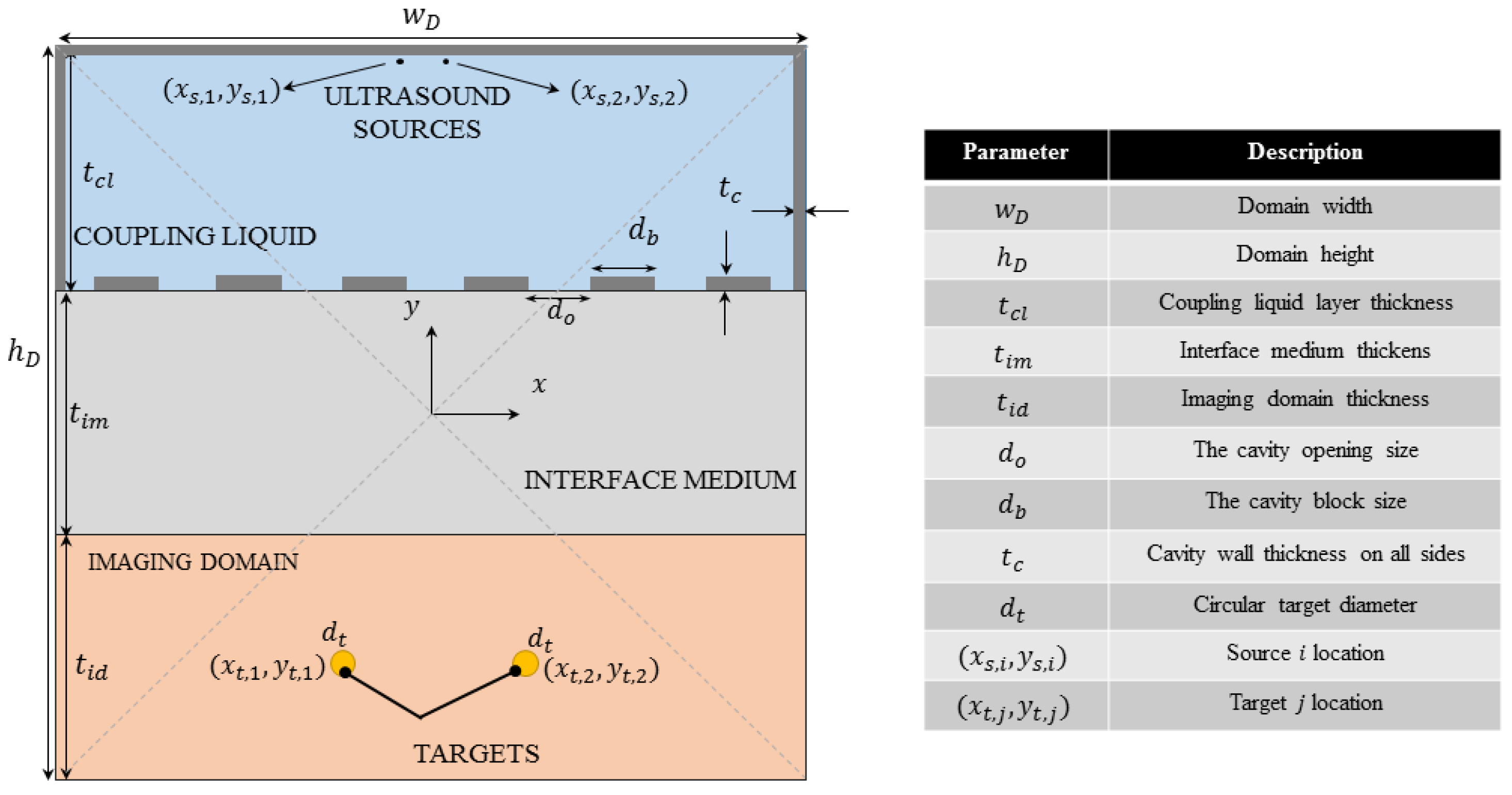
Figure 2.
The background, total and scattered pressure fields for a monopole acoustic source all satisfy the Helmholtz equation in the imaging domain, provided that the density of the scattering target is close to that of the background.
Figure 2.
The background, total and scattered pressure fields for a monopole acoustic source all satisfy the Helmholtz equation in the imaging domain, provided that the density of the scattering target is close to that of the background.

Figure 3.
(a) Sensing capacity in bits/s/Hz and (b) the amplitude of the singular values of the sensing matrix in dB for different opening sizes, in terms of , in the cavity against the case where no cavity is used. is also represented in dB.
Figure 3.
(a) Sensing capacity in bits/s/Hz and (b) the amplitude of the singular values of the sensing matrix in dB for different opening sizes, in terms of , in the cavity against the case where no cavity is used. is also represented in dB.

Figure 4.
Comparing the sensing capacity difference (%) of the steel, aluminum and VeroWhitePlus cavities with the no-cavity case in the setup shown in Figure 1. is in dB.
Figure 4.
Comparing the sensing capacity difference (%) of the steel, aluminum and VeroWhitePlus cavities with the no-cavity case in the setup shown in Figure 1. is in dB.

Figure 5.
Wave pattern coding using the aluminum cavity around the transceivers. Different and psuedo-random modes are excited at each frequency due to the presence of the holey cavity and the interaction of the waves with it. The pressure units are in pascals, and the amplitude of the source excitation was set to be 1 Pa. X and Y are in mm.
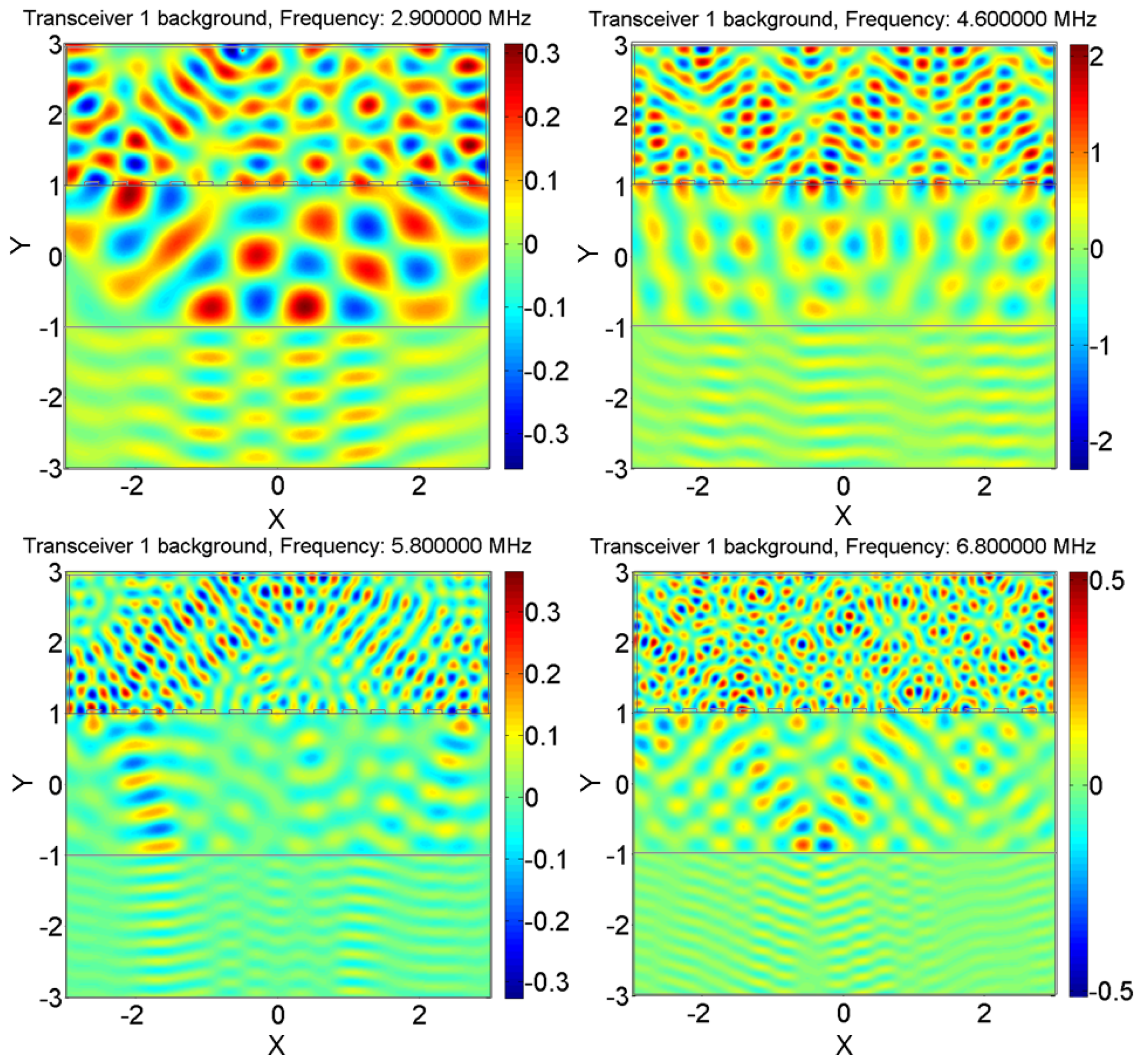
Figure 6.
The PSF when the phase-based focused beam is formed at (−0.6,−2) mm and (0.8,−2) mm on the left and right side, respectively: without a cavity, with the plastic cavity and with the aluminum cavity (from top to bottom). Focusing is strongly improved in the case of the aluminum cavity. The unit of focused beams is in pascals, and X and Y are in mm. It should be noted, as described in Section 3.4, that these PSFs are formed using the background fields without any targets present.

Figure 7.
Imaging of the point-like targets with the Hermitian of the sensing matrix and with the ADMM: without the cavity, with the plastic cavity and with the aluminum cavity. Measurement randomization has enhanced the cross-range resolutions in both cases of the plastic and aluminum cavity, but more effectively in the later case than the former. The addition of the aluminum cavity has introduced a weak artifact beside the left target; yet, the location of both targets is clear, showing the maximum intensity. These graphs illustrate the retrieval results of the contrast variable, which is unitless. X and Y are in mm. The ADMM input parameters (Algorithm 1) are also presented at the top of each ADMM image.
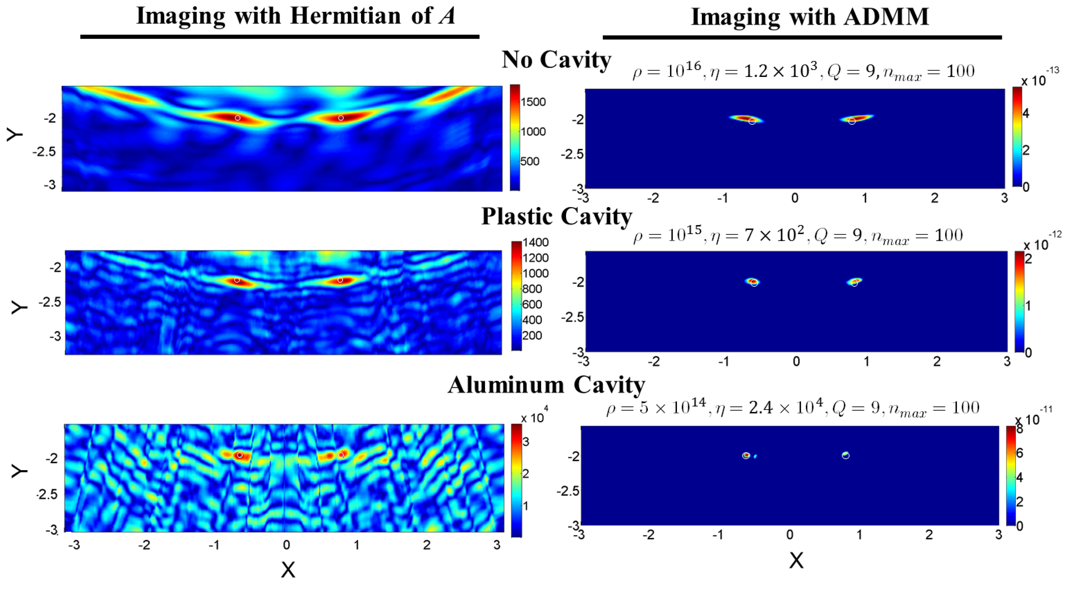
Figure 8.
(a) The multiplication of the sensing matrix by its Hermitian, normalized to have a maximum value of one (as the criterion for the quality of approximation), and (b) the convergence plot of the ADMM images presented in semi-log format for a better view of the values. The convergence plots show that the difference between the absolute value of and (refer to Algorithm 1) quickly decreases to relatively minute values, which ensures reaching the convergent solution. The convergence of the solution of the cavities case shows some noticeable oscillations, which are permissible, as they are small relative to the final error value.
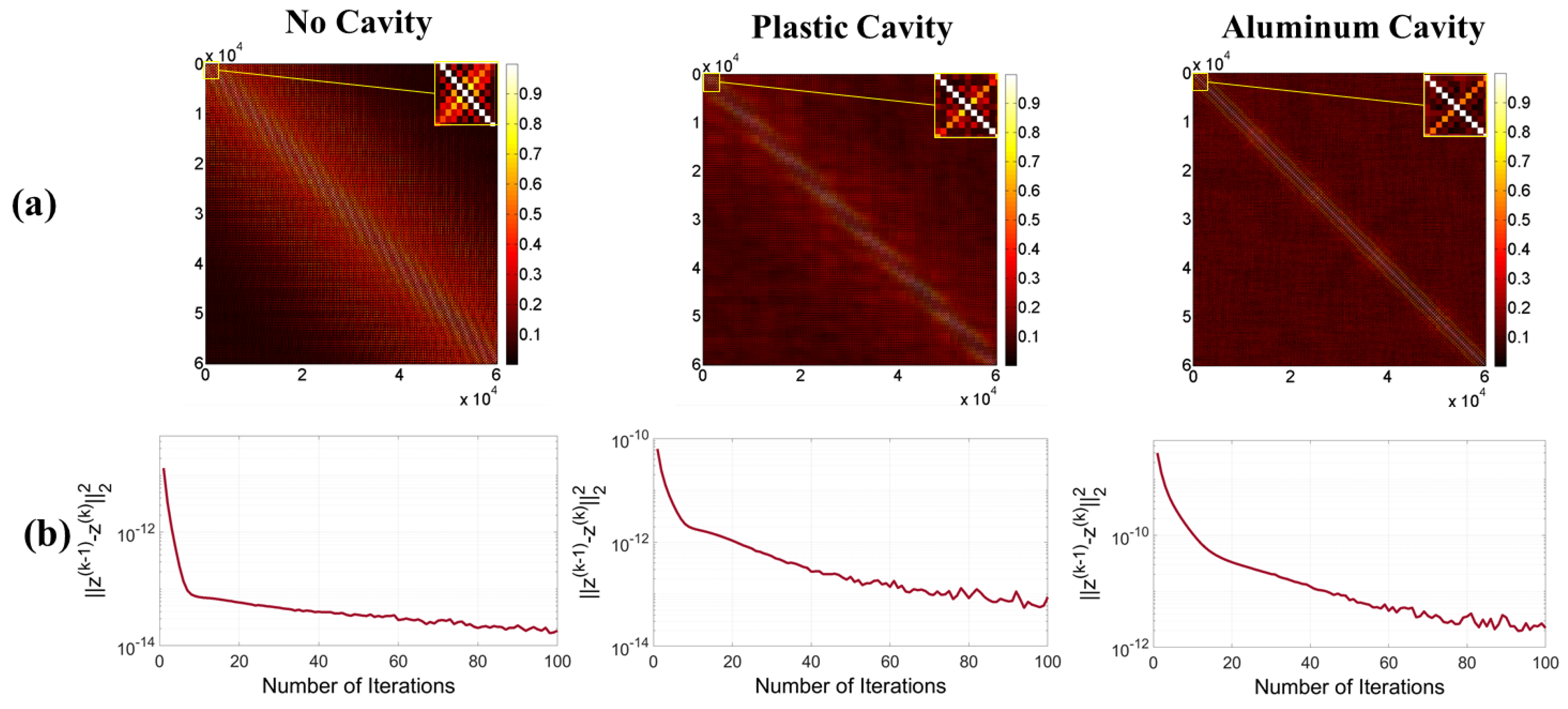
Figure 9.
Inspection of the retrieved signals at mm and their comparison with the known ground truth. The relative half-power width of the signals’ main lobes on the left and right are computed with respect to the width of the main lobes of the ground truth signal. The outcomes are presented at the top-left of the plot, showing that the aluminum cavity, despite having side lobes, leads to the best cross-range resolution among the others. Using this cavity has also outperformed other methods in terms of the relative error generated in the target center position.
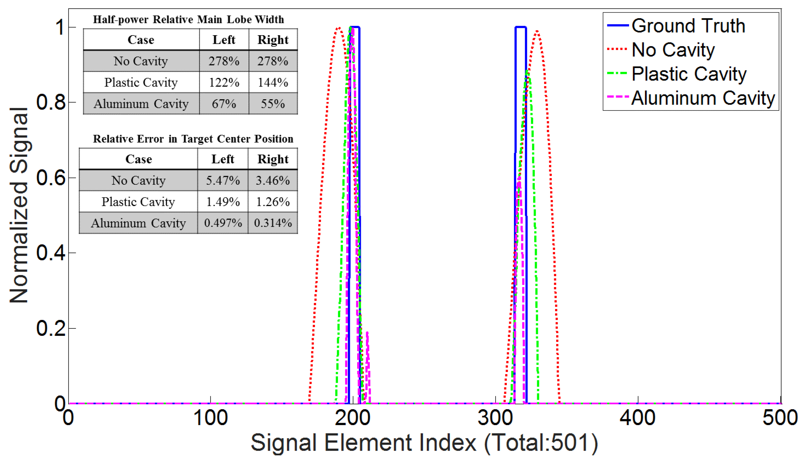
Figure 10.
The study of adding noise to the measurements: rows showing the ADMM imaging results with different s of 20 dB, 15 dB and 10 dB and columns showing different case studies. With this configuration, the plastic cavity is the most adaptive to noise.
Figure 10.
The study of adding noise to the measurements: rows showing the ADMM imaging results with different s of 20 dB, 15 dB and 10 dB and columns showing different case studies. With this configuration, the plastic cavity is the most adaptive to noise.


Table 1.
The acoustic properties of the materials used in the simulations.
| Material | Density | Longitudinal Speed of Sound | Reference |
|---|---|---|---|
| Acrylic (PMMA) | 1200 kg/m | 2730 m/s | [43,44] |
| Background | 1035 kg/m | 1487 m/s | [45,46] |
| Target | 1077 kg/m | 1549 m/s | [47,48] |
| Steel | 7700 kg/m | 5050 m/s | [49] |
| Aluminum | 2730 kg/m | 6800 m/s | [49] |
| VeroWhitePlus | 1175 kg/m | 2539 m/s | [50,51] |
Table 2.
The geometric values used in the simulations.
| Parameter | Value | Parameter | Value |
|---|---|---|---|
| 6 mm | 6 mm | ||
| 2 mm | 2 mm | ||
| 2 mm | 0.05 mm | ||
| 0.1 mm | (−0.5, 2.9) mm | ||
| (0.5, 2.9) mm | (−0.6, −2) mm | ||
| (0.8, −2) mm | 501 | ||
| 120 |
© 2018 by the authors. Licensee MDPI, Basel, Switzerland. This article is an open access article distributed under the terms and conditions of the Creative Commons Attribution (CC BY) license (http://creativecommons.org/licenses/by/4.0/).
Share and Cite
MDPI and ACS Style
Ghanbarzadeh-Dagheyan, A.; Liu, C.; Molaei, A.; Heredia, J.; Martinez Lorenzo, J. Holey-Cavity-Based Compressive Sensing for Ultrasound Imaging. Sensors 2018, 18, 1674. https://doi.org/10.3390/s18061674
AMA Style
Ghanbarzadeh-Dagheyan A, Liu C, Molaei A, Heredia J, Martinez Lorenzo J. Holey-Cavity-Based Compressive Sensing for Ultrasound Imaging. Sensors. 2018; 18(6):1674. https://doi.org/10.3390/s18061674
Chicago/Turabian StyleGhanbarzadeh-Dagheyan, Ashkan, Chang Liu, Ali Molaei, Juan Heredia, and Jose Martinez Lorenzo. 2018. "Holey-Cavity-Based Compressive Sensing for Ultrasound Imaging" Sensors 18, no. 6: 1674. https://doi.org/10.3390/s18061674
Note that from the first issue of 2016, this journal uses article numbers instead of page numbers. See further details here.