Evaluation of the Continuous Wavelet Transform for Detection of Single-Point Rub in Aeroderivative Gas Turbines with Accelerometers


Abstract
1. Introduction
2. Materials and Methods
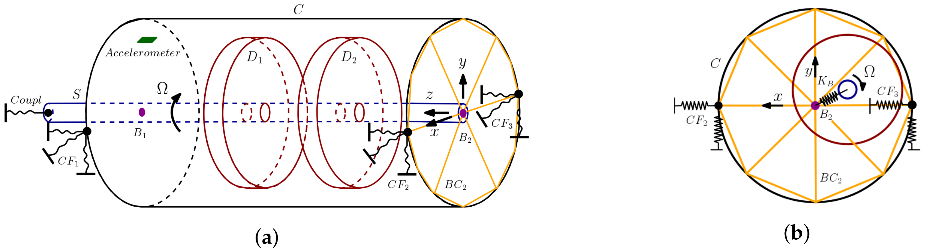
2.1. Rotor–Casing Model
2.1.1. Rotor Unbalance
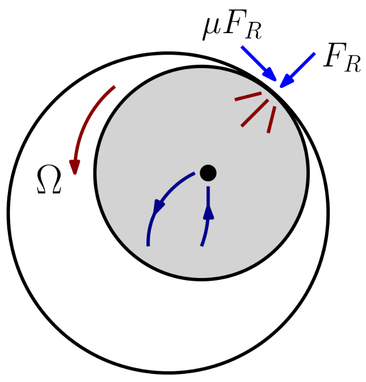
2.1.2. Rub Forces
2.2. Model Reduction and Integration
2.2.1. The Craig–Bampton Method
2.2.2. The Newmark- Methbd
2.3. Signal Extraction and Processing
2.3.1. Fourier Analysis
2.3.2. Real Cepstrum
2.3.3. Continuous Wavelet Transform
3. Results
3.1. Fourier Analysis
3.2. Real Cepstrum
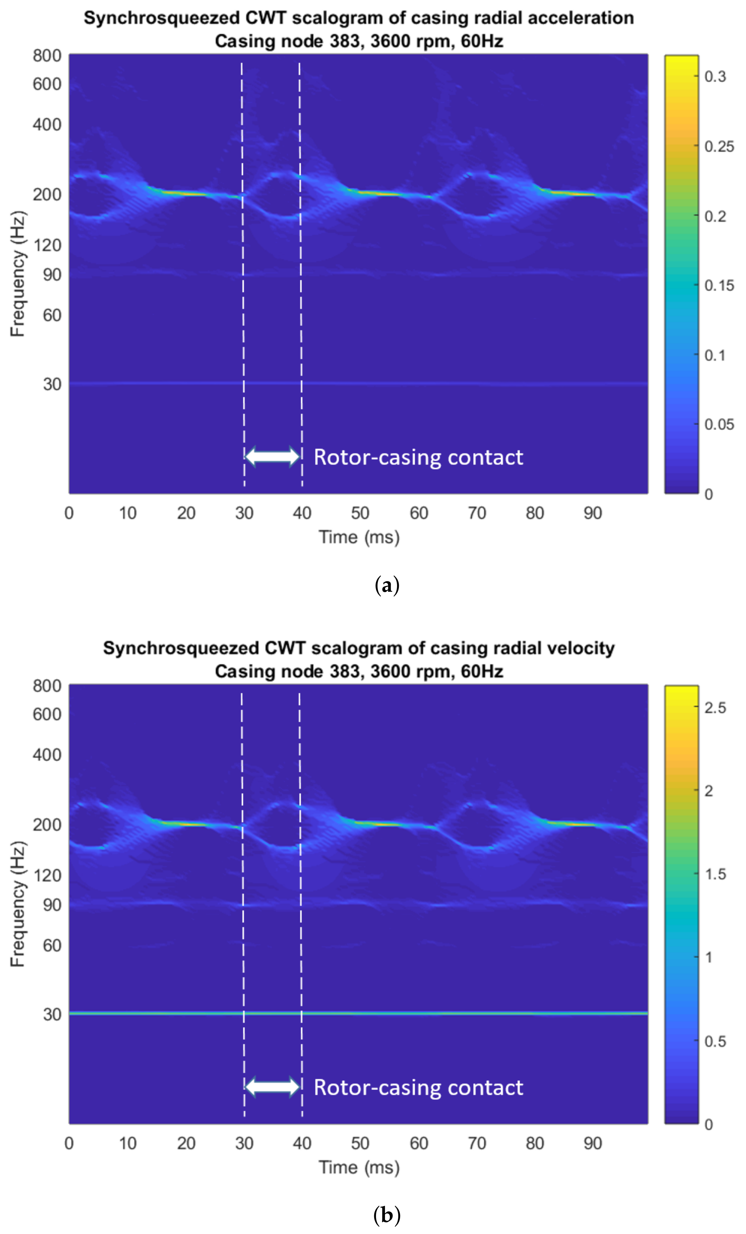
3.3. Continuous Wavelet Transform
Detection Times with DFT/FFT and CWT
4. Discussion
Author Contributions
Funding
Conflicts of Interest
Abbreviations
| x | Global radial horizontal axis |
| y | Global radial vertical axis |
| z | Global axial axis |
| Global mass matrix | |
| Global viscous damping matrix | |
| Rotor rotation speed | |
| Global gyroscopic matrix | |
| Global stiffness matrix | |
| Vector of global nodal displacements | |
| Vector of global nodal velocities | |
| Vector of global nodal accelerations | |
| t | time variable |
| Global unbalance forces vector | |
| Global rub forces vector | |
| Shaft and disks mass submatrix | |
| Casing mass submatrix | |
| Bearing mass submatrix | |
| Shaft and disks gyroscopic submatrix | |
| Shaft and disks viscous damping submatrix | |
| , | Viscous damping submatrices, shaft and disks-bearing coupling |
| Casing viscous damping submatrix | |
| , | Viscous damping submatrices, casing-bearing coupling |
| Casing viscous damping submatrix | |
| Shaft and disks viscous damping submatrix | |
| , | Stiffness submatrices, shaft and disks-bearing coupling |
| Casing viscous damping submatrix | |
| , | Stiffness submatrices, casing-bearing coupling |
| Bearing viscous damping submatrix | |
| Vector of global shaft and disks nodal displacements | |
| Vector of global casing nodal displacements | |
| Vector of global bearing nodal displacements | |
| Mass matrix coefficient of the Rayleigh damping equation | |
| Stiffness matrix coefficient of the Rayleigh damping equation | |
| damping factor of i-th system natural mode | |
| i-th system natural frequency | |
| Unbalance force vector at shaft node i | |
| Unbalance mass at shaft node i | |
| Unbalance mass distance to rotating axis at shaft node i | |
| Angular position of the unbalance mass at shaft node i | |
| Rub contact stiffness coefficient | |
| Rub contact damping coefficient | |
| Normal rub force | |
| Rub friction coefficient | |
| Unitary vector normal to shell midplane at casing node j | |
| Relative displacement between rotor and rub obstacle | |
| Relative velocity between rotor and rub obstacle | |
| , | Radial displacements of shaft node i |
| , | Radial displacements of casing node j |
| , | Radial velocities of shaft node i |
| , | Radial velocities of casing node j |
| Clearance between rotor and rub obstacle | |
| Casing midplane radius | |
| Rotor radius at shaft node i | |
| , | Rub force vectors at shaft and casing nodes i and j |
| Angle of the unitary vector normal to shell midplane with respect to x | |
| Vector of samples | |
| Vector of Fourier coefficients | |
| Signal in the time domain | |
| Fourier transform operator | |
| Inverse Fourier transform operator | |
| Cepstrum of a signal | |
| Mother wavelet function | |
| a | Dilation factor of the Wavelet transform |
| b | Translation factor of the Wavelet transform |
| Wavelet coefficient | |
| E | Young modulus |
| I | Second moment of area |
| Shaft length between bearings | |
| Boundary degrees of freedom | |
| Internal degrees of freedom | |
| Vector of external forces at the boundary degrees of freedom | |
| Vector of external forces at the internal degrees of freedom | |
| , , , | Submatrices of the reordered mass matrix |
| , , , | Submatrices of the reordered gyroscopic matrix |
| , , , | Submatrices of the reordered viscous damping matrix |
| , , , | Submatrices of the reordered stiffness matrix |
| Craig–Bampton reduction matrix | |
| Vector of modal internal degrees of freedom | |
| Submatrix of constrained modes | |
| Submatrix of matrix modes | |
| Diagonal matrix of eigenvalues | |
| Reduced mass matrix | |
| Reduced gyroscopic matrix | |
| Reduced viscous damping matrix | |
| Reduced stiffness matrix | |
| Reduced unbalance forces vector | |
| Reduced rub forces vector | |
| Reduced global rub forces vector |
Appendix A. Description of the Craig–Bampton Method
References
- Muszynska, A. Rotordynamics; CRC Press: Boca Ratón, FL, USA, 2003; ISBN 9780824723996. [Google Scholar]
- Bently, D.E.; Hatch, C.T. Fundamentals of Rotating Machinery Diagnostics; Bently Pressurized Bearing Press: Minden, NV, USA, 2002; ISBN 978-0971408104. [Google Scholar]
- Chen, G. Characteristics analysis of blade-casing rubbing based on casing vibration acceleration. J. Mech. Sci. Technol. 2015, 29, 1513–1526. [Google Scholar] [CrossRef]
- Chen, G. Study on the recognition of aero-engine blade-casing rubbing fault based on the casing vibration acceleration. Measurement 2015, 65, 71–80. [Google Scholar]
- Yu, M.; Jiang, G.; Wang, W. Aero-engine rotor-static rubbing characteristic analysis based on casing acceleration signal. J. Vibroeng. 2015, 17, 4180–4192. [Google Scholar]
- Chen, G. Simulation of casing vibration resulting from blade-casing rubbing and its verifications. Measurement 2016, 361, 190–209. [Google Scholar] [CrossRef]
- Chen, G. Vibration modelling and verifications for whole aero-engine. J. Sound Vib. 2015, 349, 163–176. [Google Scholar] [CrossRef]
- Wang, N.F.; Jiang, D.X.; Han, T. Dynamic characteristics of rotor system and rub-impact fault feature research based on casing acceleration. J. Vib. 2016, 18, 1525–1539. [Google Scholar]
- Randall, R.B. A history of cepstrum analysis and its application to mechanical problems. Mech. Syst. Signal Process. 2017, 97, 3–19. [Google Scholar] [CrossRef]
- Kovacevic, J.; Goyal, V.K.; Vetterli, M. Fourier and Wavelet Signal Processing. Chapter 6, Section 5. Available online: http://www.fourierandwavelets.org/ (accessed on 28 December 2017).
- Yan, R.; Gao, R.X.; Chen, X. Wavelets for fault diagnosis of rotary machines: A review with applications. Signal Process. 2014, 96, 1–15. [Google Scholar] [CrossRef]
- Yang, Y.; Cao, D.; Yu, T.; Wang, D.; Li, C. Prediction of dynamic characteristics of a dual-rotor system with fixed point rubbing—Theoretical analysis and experimental study. Int. J. Mech. Sci. 2016, 115, 253–261. [Google Scholar] [CrossRef]
- Jones, S. Finite Elements for the Analysis of Rotor-Dynamic Systems that Include Gyroscopic Systems. Ph.D. Thesis, Brunel University, Uxbridge, UK, 2005. [Google Scholar]
- Muszynska, A. Rotordynamics; CRC Press: Boca Ratón, FL, USA, 2003; Chapter 3; ISBN 9780824723996. [Google Scholar]
- Ahmad, S.; Irons, B.M.; Zienkiewicz, O.C. Analysis of thick and thin shell structures by curved finite elements. Int. J. Numer. Methods Eng. 1970, 2, 419–451. [Google Scholar] [CrossRef]
- Ma, H.; Shi, C.; Han, Q.; Wen, B. Fixed-point rubbing fault characteristic analysis of a rotor system based on contact theory. Mech. Syst. Signal Process. 2013, 38, 137–153. [Google Scholar] [CrossRef]
- Behzad, M.; Alvandi, M.; Mba, D.; Jamali, J. A finite element-based algorithm for rubbing induced vibration prediction in rotors. J. Sound Vib. 2013, 332, 5523–5542. [Google Scholar] [CrossRef]
- Ma, H.; Wu, Z.; Tai, X.; Wen, B. Dynamic characteristics analysis of a rotor system with two types of limiters. Int. J. Mech. Sci. 2014, 88, 192–201. [Google Scholar] [CrossRef]
- Mokhtar, M.A.; Darpe, A.K.; Gupta, K. Investigations on bending-torsional vibrations of rotor during rotor-stator rub using Lagrange multiplier method. J. Sound Vib. 2017, 401, 94–113. [Google Scholar] [CrossRef]
- Craig, R.; Bampton, M. Coupling of substructures for dynamic analyses. AIAA J. 1968, 6, 1313–1319. [Google Scholar]
- Newmark, N.M. A method of computation for structural mechanics. J. Eng. Mech. Div. 1959, 85, 67–94. [Google Scholar]
- Vetterli, M.; Kovačević, J.; Goyal, V.K. Foundations of Signal Processing; Cambridge University Press: Cambridge, UK, 2014; Chapter 3; ISBN 978-1107038608. [Google Scholar]
- Cooley, J.W.; Tukey, J.W. An algorithm for the machine calculation of complex Fourier series. Math. Comput. 1965, 19, 297–301. [Google Scholar] [CrossRef]
- Ashmead, J. Morlet wavelets in quantum mechanics. Quanta 2012, 1, 58–70. [Google Scholar] [CrossRef]
- Lin, J.; Qu, L. Feature extraction based on Morlet wavelet and its application for mechanical fault diagnosis. J. Sound Vib. 2000, 234, 135–148. [Google Scholar] [CrossRef]
- Zheng, H.; Li, Z.; Chen, X. Gear fault diagnosis based on continuous wavelet transform. Mech. Syst. Signal Process. 2002, 16, 447–457. [Google Scholar] [CrossRef]
- Wu, J.D.; Chen, J.C. Continuous wavelet transform technique for fault signal diagnosis of internal combustion engines. NDT E Int. 2006, 39, 304–311. [Google Scholar] [CrossRef]
- Rafiee, J.; Rafiee, M.A.; Tse, P.W. Application of mother wavelet functions for automatic gear and bearing fault diagnosis. Expert Syst. Appl. 2010, 37, 4568–4579. [Google Scholar] [CrossRef]
- Su, W.; Wang, F.; Zhu, H.; Zhang, Z.; Guo, Z. Rolling element bearing faults diagnosis based on optimal Morlet wavelet filter and autocorrelation enhancement. Mech. Syst. Signal Process. 2010, 25, 1458–1472. [Google Scholar] [CrossRef]
- Tang, B.; Liu, W.; Song, T. Wind turbine fault diagnosis based on Morlet wavelet transformation and Wigner-Ville distribution. Renew. Energy 2010, 35, 2862–2866. [Google Scholar] [CrossRef]
- Kankar, P.K.; Sharma, S.C.; Harsha, S.P. Fault diagnosis of ball bearings using continuous wavelet transform. Appl. Soft Comput. 2011, 11, 2300–2312. [Google Scholar] [CrossRef]
- Daubechies, I.; Lu, J.; Wu, H.T. Synchrosqueezed wavelet transforms: An empirical mode decomposition-like tool. Appl. Comput. Harmon. Anal. 2011, 30, 243–261. [Google Scholar] [CrossRef]
- Pennacchi, P.; Bachschmid, N.; Tanzi, E. Light and short arc rubs in rotating machines: Experimental tests and modelling. Mech. Syst. Signal Process. 2009, 23, 2205–2227. [Google Scholar] [CrossRef]
- Littrell, N. Selecting the right sensors for your machine. Orbit Mag. 2013, 33, 46–53. [Google Scholar]
- Tang, B.; Liu, W.; Song, T. Numerical investigations on axial and radial blade rubs in turbo-machinery. Nonlinear Dyn. 2016, 84, 1225–1258. [Google Scholar]


| Shaft length: | 0.6 m | Young modulus of shaft: | Pa |
| Distance between shaft bearings: | 0.4 m | Shaft density: | 7850 kg m |
| Shaft diameter: | 0.01 m | Casing density: | 1600 kg m |
| Disk mass: | 1.5 kg | Young modulus of casing: | 7 Pa |
| Disk thickness: | 0.025 m | Poisson’s ratio of casing: | 0.1 |
| Disk diameter: | 0.1 m | Bearing radial direct stiffness: | N m |
| Casing midplane diameter: | 0.134 m | Casing support stiffness: | N m |
| Casing length: | 0.4 m | Bearing-casing truss bar stiffness: | N m |
| Casing thickness: | 0.003 m | Bearing mass: | 0.02 kg |
| Time for Data Acquisition | Time for Data Processing | Total Time | ||
|---|---|---|---|---|
| Acceleration data | 2 s | 0.001172 s | 2.00117 s | |
| DFT/FFT | Velocity data | 2 s | 0.000132 s | 2.00013 s |
| Acceleration data | 0.1 s | 0.026428 s | 0.12643 s | |
| CWT | Velocity data | 0.1 s | 0.009997 s | 0.11000 s |
© 2018 by the authors. Licensee MDPI, Basel, Switzerland. This article is an open access article distributed under the terms and conditions of the Creative Commons Attribution (CC BY) license (http://creativecommons.org/licenses/by/4.0/).
Share and Cite
Silva, A.; Zarzo, A.; Munoz-Guijosa, J.M.; Miniello, F. Evaluation of the Continuous Wavelet Transform for Detection of Single-Point Rub in Aeroderivative Gas Turbines with Accelerometers. Sensors 2018, 18, 1931. https://doi.org/10.3390/s18061931
Silva A, Zarzo A, Munoz-Guijosa JM, Miniello F. Evaluation of the Continuous Wavelet Transform for Detection of Single-Point Rub in Aeroderivative Gas Turbines with Accelerometers. Sensors. 2018; 18(6):1931. https://doi.org/10.3390/s18061931
Chicago/Turabian StyleSilva, Alejandro, Alejandro Zarzo, Juan M. Munoz-Guijosa, and Francesco Miniello. 2018. "Evaluation of the Continuous Wavelet Transform for Detection of Single-Point Rub in Aeroderivative Gas Turbines with Accelerometers" Sensors 18, no. 6: 1931. https://doi.org/10.3390/s18061931
APA StyleSilva, A., Zarzo, A., Munoz-Guijosa, J. M., & Miniello, F. (2018). Evaluation of the Continuous Wavelet Transform for Detection of Single-Point Rub in Aeroderivative Gas Turbines with Accelerometers. Sensors, 18(6), 1931. https://doi.org/10.3390/s18061931