DNN-MVL: DNN-Multi-View-Learning-Based Recover Block Missing Data in a Dam Safety Monitoring System


College of Computer and Information, Hohai University, Nanjing 211100, China
*
Authors to whom correspondence should be addressed.
Sensors 2019, 19(13), 2895; https://doi.org/10.3390/s19132895
Submission received: 10 June 2019
/
Revised: 22 June 2019
/
Accepted: 25 June 2019
/
Published: 30 June 2019
(This article belongs to the Special Issue Algorithm and Distributed Computing for the Internet of Things)
Abstract
:Many sensor nodes have been widely deployed in the physical world to gather various environmental information, such as water quality, earthquake, and huge dam safety. Due to the limitation in the batter power, memory, and computational capacity, missing data can occur at arbitrary sensor nodes and time slots. In extreme situations, some sensors may lose readings at consecutive time slots. The successive missing data takes the side effects on the accuracy of real-time monitoring as well as the performance on the data analysis in the wireless sensor networks. Unfortunately, existing solutions to the missing data filling cannot well uncover the complex non-linear spatial and temporal relations. To address these problems, a DNN (Deep Neural Network) multi-view learning method (DNN-MVL) is proposed to fill the successive missing readings. DNN-MVL mainly considers five views: global spatial view, global temporal view, local spatial view, local temporal view, and semantic view. These five views are modeled with inverse distance of weight interpolation, bidirectional simple exponential smoothing, user-based collaborative filtering, mass diffusion-based collaborative filtering with the bipartite graph, and structural embedding, respectively. The results of the five views are aggregated to a final value in a multi-view learning algorithm with DNN model to obtain the final filling readings. Experiments on large-scale real dam deformation data demonstrate that DNN-MVL has a mean absolute error about 6.5%, and mean relative error 21.4%, and mean square error 8.17% for dam deformation data, outperforming all of the baseline methods.
1. Introduction
Many wireless sensor networks (WSNs) have been widely deployed in the physical world to sense and collect various environmental information or events, such as water quality [1], air quality [2], forest fire [3], and dam safety [4]. These sensors generate massive geo-tagged time series data, helping humans to make further analysis and decision [5]. However, affected by hardware and severe wireless conditions, such as strong fade in WSNs, raw sensory data can have loss and corruption. Due to the limitation in the battery power, memory, and computational capacity, the readings generated from sensors are unreliable or inaccurate [6,7,8,9]. In addition, some sensors may malfunction and result in faulty and missing data in the unattended situations. Massive missing readings in the WSNs will not only affect real-time monitoring especially for emergency conditions, but also compromise the performance of further data analysis and decision. It is extremely important to obtain the full and accurate monitoring data from raw readings before making any further analysis and decision. Considering the internal and external factors, events occurred in the physical world cannot be accurately detected using inaccurate and incomplete sensory data [10]. Therefore, it is necessary to complete the missing reading from a large-scale wireless sensor network with geo-sensory time series data.
Several solutions have been proposed to handle block missing data, such as K-nearest neighbors-based local interpolation [11], Kriging interpolation [12], and multi-channel singular spectrum analysis (MSSA) based on PCA (Principal Component Analysis) [13]. Unfortunately, those methods cannot well establish the spatial-temporal correlations, which results in the fair-quality interpolation. Moreover, matrix completion (MC) methods have been applied to fill the missing reading from partially observed geo-sensory data [14,15]. Different the interpolation methods, matrix completion often seeks to find the lowest rank matrix or well matches the known entries of a matrix with missing data. Matrix completion techniques can be utilized for filling the random missing readings. However, when there exist block missing readings along the column or the row due to sensor failures, it is very difficult to find stable inputs for the matrix completion model. Some global initialization methods have been proposed to avoid the unstable inputs for the matrix completion. For example, non-negative matrix factorization based on the multi-view [16,17], the user-based collaborative filtering [18], and matrix factorization and a salient version called empirical orthogonal functions model [19,20,21,22] can be applied to fill missing values. Although those methods consider the spatial-temporal views, they just adopt the linear fusion model with multiple views results, which cannot generate more accurate estimate for filling missing data.
Missing data can occur at arbitrary sensor nodes and time slots. In extreme situations, some sensors may lose readings at consecutive time slots. In this paper, the dam deformation observation dataset is from the real Dam Safety Monitoring Systems, recording the observation values from 2017/01/01 to 2017/12/31. There are five sensor nodes for monitoring the dam deformation P02023, P04615, P04616, P04617, and P06656, represented as , , , , and , respectively shown in Figure 1. From Figure 1a,b, three sensors P04616, P04615, P04617 are closely deployed in the spatial space, while the spatial distribution between two sensors P02023, and P06656 is far away. As illustrated in Figure 1c, four sensor nodes lost their readings in the time slot . Meanwhile, sensor node cannot record the observed readings from the time slot and , which is called as block missing.
On the other hand, affected by multiple complex factors, sensor readings vary with the locations and time significantly and non-linearly. The observed data of sensors with a shorter distance may not always be more similar than those with a farther distance. For example, Figure 2 shows the observed data of five sensors from 1 January 2017 to 31 December 2017. From Figure 2a,b, the distance between two sensors P02023 and P06656 is much farther than the distance between two sensors P04615 and P04617. However, the readings of P02023 and P06656 are more similar than those of P04615 and P04617. The reason is that two sensors P02023 and P06656 are in two different regions with similar mechanical structure. This case violates the First Law of Geography: “near things are more related than distant things.” Furthermore, sensor readings sometimes exhibit a sudden change, as illustrated in Figure 2. The readings of sensor P02023 from 10 August 2017 to 14 August 2017. Such a sudden change may have a side effect on the real-time monitoring and data analysis. Existing interpolation-based and smoothing methods cannot obtain good results.
Filling block missing reading from a large-scale sensor network with geo-sensory time series data is a challenging task. To solve the above problem, a unified multi-view-learning model in a deep learning model (DNN-MVL) is proposed to fill the block missing values that jointly consider the spatial relations between different time series from the different sensor nodes, and the temporal relations between readings at different time slots in the same series from one node, and semantic correlations through graph embedding. We conducted extensive experiments on real dam deformation monitoring dataset and Beijing air quality dataset. The results demonstrate that the proposed method DNN-MVL can achieve high filling accuracy in the presence of block missing data.
The rest of this paper is organized as follows. We introduce the related work in Section 2. The preliminary and problem statement are presented in Section 3. The main framework of the proposed DNN-MVL is introduced in Section 4. In Section 5, we present our proposed DNN-MVL approach for filling the block missing data. Finally, we evaluate the performance of the proposed DNN-MVL with Beijing air quality data and large-scale real dam deformation data in Section 6, and conclude the work in Section 7.
2. Background and Related Work
Data missing is unavoidable problem during the data transmission and collection in the wireless sensor networks. To solve the data missing problem, existing solutions can be classified into two types: (1) the missing data is deleted from the time series. (2) The missing data is filled with an estimation with the interpolation model based on the historical data. It is a simple way to delete the missing readings from the time series. However, it may result in the poor data quality when deleting successive data missing. The missing reading filling is a better approach with interpolation or matrix completion.
A lot of work has been focused on the interpolation for the missing data. K-nearest-neighbor (KNN) [23] is a simple local interpolation method that utilizes the values of the nearest K neighbors to estimate its missing value. KNN is only applied for data interpolation with very few missing values. Unfortunately, it performs poorly for the blocking missing. Meanwhile, the sensory data from WSNs are usually the time series. The temporal correlation model can be used to fill the missing data. Auto-regressive integrated moving average model (ARIMA) is a well-known time series prediction method, which combines moving average and autoregressive components [24]. ARIMA is suitable to predict a missing value just solely considering a sensor’s readings [25]. In addition, sensor nodes are deployed in the different locations. Different geo-tagged time series data exhibit the spatial correlation. Inverse distance weighting (IDW), linear regression, and Kriging [26,27] are widely used spatial models. For example, IDW is applied to estimate the rainfall distribution [28], and Kriging is used to fill the missing temperature [29]. Those models can be used to interpolate a missing value with available readings in the spatial correlation. While those studies still fail to capture the complex non-linear spatial-temporal correlations.
Besides the above methods, matrix completion (MC) methods have emerged and been applied to fill the missing reading from partially observed geo-sensory data [30,31]. Different from the interpolation methods, matrix completion often seeks to find the lowest rank matrix or, if the rank of the completed matrix is known, which well matches the known entries of a matrix with missing data. Matrix completion techniques can be utilized for filling the random missing readings due to the unreliable wireless transmissions, if exploiting the spatial-temporal correlations. However, when there exist block missing readings along the column or the row due to fading or sensor failures, it is very difficult to find stable inputs for the matrix completion model.
Recently, there are many data-driven methods from multiple views for filling missing values were proposed. To model the spatial-temporal correlation, a data estimation for mobile sensors method was presented to fill the missing data through establishing the time-dependent spatial-temporal correlation in the mobile wireless sensor networks [32,33]. When there is not enough spatial and temporal information, a spatial and temporal K-nearest neighbors (ST-KNN) imputation method adopted the weighted average to fill the missing values [34]. In the recommendation system, user-based and item-based collaborative filtering methods were introduced to fill missing values considering the users similarity and temporal similarity [35]. However, when meeting the sparse matrix problem, it is difficult to generate the accurate the filling values due to the inaccurate results of similarity. Considering spatial, temporal, global and local views, combining the statistic models and data-driven models in a spatial–temporal multi-view learning (ST-MVL) framework was established to generate a more accurate estimate [20]. These studies on the multiple view learning methods are mainly based on the linear fusion from different views to estimate the missing values. They fail to model the complex non-linear relations of the space and time.
In summary, the difference of our proposed method DNN-MVL compared with other work is that we consider the spatial correlation, temporal sequence correlation and functional correlation in a joint deep learning model.
3. Problem Statement
In this section, we first fix some notations and present the problem formulation. In the WSNs, the data collected from the monitoring of the dynamic environment can generally be represented by a matrix, defined as . The matrix records data from sensors over time slots, in which represents the sensors’ readings and represents the consecutive time slots. As shown in Figure 3, in the matrix , a row stands for a sensor and a column denotes a time slot. An entry represents the readings of the sensor at the time slot . Due to hardware failure or severe transmission condition in the WSNs, the measured and collected data are often unreliable. As a result, both the matrix rows and columns in the sensory matrix may have some successive missing data, as shown in Figure 3. In this paper, we call it a block missing problem. The filling missing data problem aims to fill the readings at time interval given the data until the time interval.
Since the observed data in WSNs normally have strong correlation between neighboring locations and timestamp, we can incorporate temporal views, spatial views, and functional (semantic) views to fill the missing readings of sensors. Therefore, in order to fill the block missing readings, we propose DNN-MVL method to collectively consider the global-local, spatial-temporal, and semantic views simultaneously to fill the missing readings. The results of the five views are aggregated to a final value in a multi-view learning algorithm with DNN model.
4. Main Idea
To capture the complex and non-linear spatial-temporal correlations when filling the block missing values, DNN-based multiple view learning framework was proposed. The temporal view establishes the sequential relations model in the time series and estimates the missing values of a sensor based on the readings at the neighbor time slots of the same sensor node. The readings of sensors are often smooth in a small spatial area. The recorded data at nearby locations have similar values at a given time. The spatial view can estimate a missing value based on the spatial similarity between a sensor’s current readings and those of sensors’ spatial neighbors. Furthermore, different time length of the observed data for filling missing readings can be considered as global view and local view. For example, if an entry is lost, we can use the adjacent readings of sensor from to to fill the missing readings, which is called as a temporal local view. Likewise, we also estimate the reading of based on the its spatial neighbors and , which is a spatial local view. Obviously, local view can capture the instantaneous changes. We can consider the readings over a long time period from to to recover the missing value, which is regarded as a global view. Global views can represent the long-term patterns. In general, the sensors with similar functionality may have similar patterns, e.g., at both ends of the arch dam may have similar structural mechanics. Similar regions may not necessarily be close in space. Therefore, the structural embedding method is applied to construct a graph of sensors’ locations representing functional similarity among the sensors in the different regions. In this paper, semantic similarity is equal to functional similarity.
Our proposed DNN-MVL framework includes five views, as shown in Figure 4. Global spatial view with inverse distance weighting interpolation can compute an estimated value of a missing reading based on the values of the sensors’ spatial neighbors. Global temporal view with bidirectional simple exponential smoothing is used for analysis of time series data. Exponential smoothing is a prediction model derived from amount of historical data using the exponential window function to assign exponentially decreasing weights over time. From the local spatial view, if a sensor node is regarded as a user, user-based collaborative filtering can predict the missing reading based on the local similarity between a sensor’s readings and those of its neighbors. Local temporal view with mass diffusion-based collaborative filtering method can estimate the missing readings based on the local similarity between recent readings at the different time slots of the same sensor. Semantic view is constructed with a graph of sensors’ locations representing the functional similarity among different locations. With the dynamic time wrapping method, the functional similarity is measured by the similarity between the time sequences originated from two sensor nodes. To leverage the results of different views for the missing readings, a deep neural network model is adopted to generate the final results of five different views’ estimations with minimal errors.
5. DNN-Based Multiple View Learning Framework
In this section, we provide details of the proposed DNN-based multiple view learning framework (DNN-MVL) for filling the block missing values. Our proposed DNN-MVL framework includes five views: global temporal view with IDW, local temporal view with simple exponential smoothing (SES), local spatial view with user-based collaborative filtering (UCF), local temporal view with mass diffusion (MD)-CF, and semantic view with structural embedding. The results of the five views are aggregated to obtain the final filling readings with DNN model.
5.1. Global Spatial View: IDW
To capture the long-term patterns in spatial relations, the inverse distance weighting interpolation (IDW)—a statistical model, is applied to interpolate a missing value based on its spatial neighbor sensors. IDW is a deterministic method for multivariate interpolation with a known scattered set of points. The closer the sensor with the available readings is to the target node, the greater the weight assigned to it. The assigned values to the missing values are calculated with a weighted average of the available readings of geospatially adjacent sensors. IDW estimates the prediction value mgs can be calculated as follows:
where is the value of sensor at the time slot , and is the number of sensors participating in filling missing data. is the spatial distance between a candidate sensor and the target sensor. is a positive parameter that affects the decay rate of a sensor’s weight by the geospatial distance. The value of varies from 0 to 1. The closer sensor’s readings can perform better filling results for a missing reading. assigns a bigger weight to closer sensor’s readings. Otherwise, the farther sensor’s readings are assigned with a smaller weight. is filling results with global spatial view.
To further illustrate the spatial correlation in the different sensors’ readings, the similarity ratio between arbitrary two sensors’ readings at the same time slot can be calculated as follows:
where and are the readings of sensor and at the time slot respectively, is the geospatial distance between two sensors and .
Figure 5a,b show the similarity ratio between two sensors P04616, P04617 and other deformation sensors in the dam safety monitoring dataset, respectively. The similarity ratio decreases as the distance between two sensors increases in most cases, which actually follows the First Law of Geography. i.e., “everything is related to everything else, but near things are more related than distant things,” which is an empirical spatial correlation in geo-sensory data. Two other sensors, P04615 and P04617, are near target sensor P04616, with geospatial distance 54 m and 64 m respectively. If it set the decay rate , the assigned weights to two sensors are 1/54 and 1/64. We can calculate an estimation with the weighted average values by Equation (1). We can estimate the missing values with Equation (1). To further illustrate the spatial correlation in the different sensors’ readings, Equation (2) is adopted to measure the similarity of two sensors in the global spatial correlation. Two equations can compute the spatial similarity from the different aspects. That motivates us to apply IDW interpolation to model the global spatial view. However, not all the sensor nodes are farther away from the target sensor, their similarities are smaller. For example, Figure 2b illustrates that the sensor P02023 is far away from sensor P06656. They have similar data pattern. In this paper, other views should be considered to obtain more accurate estimation.
5.2. Global Temporal View: SES
To consider the global temporal view, SES is utilized to estimate the missing value based on the historical data of same sensor at other time slots. SES is a prediction model in the time series domain using the exponential window function. SES computes the prediction value as follows:
where is the time slot of the missing reading, is a time interval between a candidate reading of sensor and a target reading ; is a smoothing parameter with a range of (0, 1). In general, if the time interval is smaller to the target one, will be set to a bigger weight. A smaller means a slower decay of weight over the time interval. However, the traditional SES only uses historical readings of the target time slot as input to model average exponential moving. In our method, it considers both the historical readings and successive readings of a target time slot as inputs to compute the average weighted smoothing.
Given a target time slot , the observed reading of sensor is . SES assigns a weight to each reading of the same sensor at the candidate time slot , where is the time interval between the candidate time slot and target slot. Thus, the prediction value using SES can be calculated as follows:
The SES model is inspired by the observation from time series data. Figure 6 shows the similarity ratio between arbitrary two readings at two different time slots of the same sensor in the dam deformation dataset. Each point in Figure 6 denotes the similarity ratio between the arbitrary reading and the target reading at the given time interval in the sensor P04616. As shown in Figure 6, the curve of similarity ratio decreases as the time interval increases. It is an empirical temporal correlation in time series. The readings of recent time slots are more relevant than those of distant time slots.
We use the example of dam deformation data to clearly demonstrate the performance of SES model. Suppose there is a missing reading at time slot , and the observed readings at the four adjacent time slots are (85, 75, 75, 85) respectively. If the smoothing parameter is set to 0.5, the weights for four time slots are (0.25, 0.5, 0.5, 0.25). The prediction value is 78.3 by Equation (4).
5.3. Local Spatial View: UCF
The fluctuation of dam deformation data is often smooth in a small region at a given time interval. The observed readings at nearby locations are similar. The local spatial correlation between a sensor node and its neighbors in a time slot can be measured as follows:
where is the -th row of topology matrix , is the -th column of sensory matrix . The topology matrix is defined as follows:
With the locations of all deployed sensor nodes, it can be easily to obtain the topology matrix. In Equation (5), is the total observed value of the neighbors of sensor , and is the number of ’s one-hop neighbors. means the average data value of one-hop neighbors of sensor at the time slot . Equation (5) can compute the difference between the reading of sensor and the average readings of its one-hop neighbors at a given time slot. Each element in the matrix represents whether the sensors and are one-hop neighbors. It is obvious that topology matrix has binary values to represent the relationship between two sensor nodes.
To further capture the spatial correlation between sensor nodes, UCF is motivated to model the spatial local correlation. The main idea of UCF is that similar users usually make similar scores for similar items. In the dam deformation monitoring, each sensor is regarded as one user, and one deformation reading of one sensor at a time slot is regarded as one item. The window size is adopted to normalize the different scale of different sensor nodes. The local readings matrix for sensor node and from the time slot to are and , respectively. The similarity measurement between two sensors and can be computed based on the cosine vector as follows:
where and are the observed readings of sensor and at the time slot , and are the average values of two sensors respectively; and are two time vectors of two sensors that there is no missing readings; is the time vector that two sensors and both have readings, that is .
The sensors’ similarities are calculated and sorted in descending order by Equation (7). The most similar target sensors are selected to construct the set of the nearest neighbors , where and . Then, we can calculate an estimation from local spatial view with the weighted average similarity as a weight as follows:
IDW does not hold the sudden change in global spatial correlation, e.g., the case shown in Figure 2b, while UCF can have good performance on the local spatial correlation by capturing the time-dependent spatial correlation in a small area between sensors’ readings.
5.4. Local Temporal View: MD-CF
In general, dam deformation data usually change slowly over time. To study the short-term and local temporal correlation for one sensor, we calculate the gap between each pair of adjacent readings for the same sensor in two consecutive time stamps and as follows:
where represents the observed data of sensor at the time slot . If the observed reading is not changed from the time slot to , it has . The smaller , the more stable the observed readings for sensor at the time slot .
However, sensor readings sometimes exhibit a sudden change, as illustrated in Figure 2. The readings of sensor P02023 from 10 August 2017 to 14 August 2017. In addition, the block missing of data results in the data sparsity. It is hard to calculate the data similarity from the adjacent readings for the same sensor. To fill the missing readings from the local temporal view of the same sensor, MD is introduced to item-based collaborative filtering for estimating the missing readings, where a time slot denotes an item. MD refers to the movement of matter from place to place, resulting in a net change in the mass’s location [36]. MD is an extremely common phenomenon in everyday life.
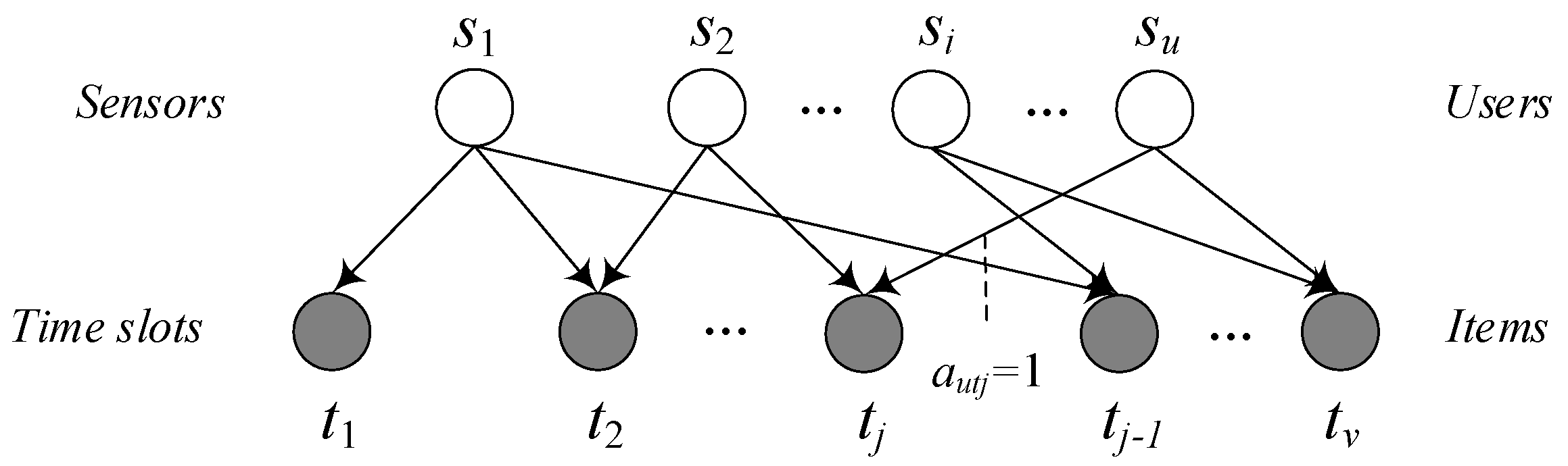
With bipartite graph, mass diffusion method can be applied to fill the missing data. In the MD-CF method, bipartite graph represents the relationship between users and items. In the bipartite graph, sensor node denotes the user and a time slot denotes an item, as shown in Figure 7. The set of sensor nodes is denoted as and the set of time slots is . If the reading of sensor node at the time slot is not missing, there has an edge between the node and . That is . Otherwise, . Thus, the bipartite graph can represent whether the sensor nodes have the missing readings at the different time slots. Through the iteration of mass diffusion, it can seek the degree of association between two nodes in the bipartite graph [37], and then it can calculate the similarity of the readings at the different time slots. The specific steps are as follows:
(1) Initialization phase. Assume that denotes the reading of node at the time slot , and is the average value of readings from the node . The initial energy at the time slot can be calculated as follows:
(2) Energy diffusion from time nodes to sensor nodes. The energy of sensor node are equally diffused to other sensor nodes which have readings at the time slot . The energy of sensor node at the time slot is denoted as , which can be calculated as follows:
where is the degree of time node in the bipartite graph, and refers to the number of sensor nodes which have the readings at the time slot . If the sensor node has readings at the time slot , it has . Otherwise, .
(3) Energy diffusion from sensor nodes to time nodes. The energy of sensor node are equally diffused to time nodes where sensor nodes have readings at the time slot based on the degree of sensor node , in which . The final energy of time node is the sum of diffused energy from all sensor nodes connected with the time node . After twice energy diffusions, the similarity of two different time slots and for the same node can be computed with the proportion of the obtained energy from the time slot to . The similarity of two different time slots can be computed as follows:
where is the degree of sensor node in the bipartite graph, the value of can be calculated with Equation (11).
(4) If the missing reading at the time slot , the adjacent time slots of are selected. Then, the similarities of all pairs of two different time slots in are calculated by Equation (12) and sorted in descending order, denoted as . That is .
(5) Adopting the CF algorithm, the weights are assigned based on the similarities. It can obtain the filling result from the local temporal view, as follows:
MD-CF method is applied to establish the time-dependent local temporal correlation learned from recent data as well as avoid the low accuracy due to the block missing.
5.5. Semantic View: Structural Embedding
Intuitively, sensor nodes sharing similar functionality may have similar data distribution. However, sensors with similar functionality may not necessarily be close in space. For example, although the spatial distance between two sensors P02023 and P06656 is not close, shown in Figure 1 and Figure 2, they have a similar data distribution. This is because their mechanical models exhibit symmetric structure. We establish a graph of sensors representing functional (semantic) similarity among sensors [38]. The semantic graph is defined as , where the set of nodes are sensors , is the edge set , and is the set of functional similarity on all of the edges. Dynamic time warping (DTW) method [39] is applied to measure the functional similarity between sensor and sensor as follows:
where is the decay parameter and is the dynamic time warping distance between the data distribution of two sensors and sensor . In the dam safety monitoring systems, we use the average seasonal deformation time series as the dam deformation patterns. The average values can be computed based on the training data in the experiment.
To fill the missing readings from the sematic view, the graph embedding method -LINE [40] is applying to extract the feature vector of the data pattern for sensor . In order to train the feature vector , the feature vector is input to a fully connected layer. Thus, we can get the filling results with training model, which is defined as:
where two parameters and are both learning parameters.
5.6. Multi-View Learning with DNN
Each view has its own feature. It does not work well if purely using global, local, or semantic views. It may obtain the better filling results if adopting multiple views fusion. The proposed DNN-MVL method integrates the estimations of the above five views to generate the final result through a multi-view learning algorithm. The linear fusion is one of the simplest solutions, however, it cannot deal with the non-linear relation among the different estimations from five views. DNN-MVL applies the DNN-based multi-view learning to fuse different predictions.
Algorithm 1 presents the procedure of DNN-MVL. When a sensor network faces a block missing problem, local spatial and temporal views cannot separately work very well. First, global spatial and temporal views (IDW and SES) are applied to generate the initial values for those missing readings, respectively. Then, five different views are used to compute the estimations for each missing entry by using IDW, SES, UCF, MD-CF, and SE, respectively. Third, it aggregates the five estimations with DNN-based multi-view learning framework to calculate the final filling value. During the procedure of deep fusion, six-layer fully connected network is used as hiding layer, and the number of cell nodes in hiding layer is 32, 64, 256, 18, 64, and 32, respectively. The activation function in the hidden layer adopts ReLU function to reduce the gradient disappearance [41]. The batch normalization is adopted to accelerate the training and convergence before the ReLU function of each layer is activated [42]. Moreover, five-fold cross-validation is used to solve the problems of over-fitting and sparse training data. Five-fold cross validation can obtain the more reliable and stable model via avoiding the noise. In the output layer, a linear activation function is applied to compute the final filling result. In the DNN-MVL, the model is optimized for each sensor respectively by minimizing the least square error between estimations and the ground truth.
| Algorithm 1: DNN_ multi-view learning method (MVL). |
| Input: Original Data Matrix ; Structure Graph ; Output: Final filling data matrix |
| 1. O ← Get-All-Missing-Values (); |
| 2. If there are successive missing readings () |
| 3. ← Initialization (); |
| 4. For each target sensor at the time slot t in O |
| 5. ← |
| 6. ← |
| 7. ← |
| 8. ← |
| 9. ← |
| 10. ← |
| 11. Add into |
| 12. Return |
6. Performance Evaluations
6.1. Datasets and Ground Truth
In this paper, the real dataset is used to evaluate the proposed DNN-MVL model. The dam safety monitor data from the highest arch dam in the world is from 2012/01/01 to 2017/08/14, which has 6159 timestamps respectively. In the experiments, 964 sensor nodes are selected from the dam safety monitor systems. Each of node generates a reading every four hours, as depicted in Figure 1. From the dataset, we fill the missing values whose statistics are shown in Table 1. There are two missing situations: block missing and general missing. The block missing is comprised of spatial block missing and temporal missing. The two-block missing may have some overlap. The spatial block missing is referred to as the reading values of all sensors simultaneously absent. The temporal block missing is the values of the same sensor with data absent in a certain temporal window size. As shown in Table 1, there are 4.6% of missing values in dam-deformation property when . General missing is the missing values except for the block missing. For example, about 15.2% of sensor readings in the Dam-Deformation dataset, including 8.4% general missing and 2.7% spatial block missing.
6.2. Data Preprocessing
In the experiment, the one-year data is partitioned into two parts. The data in March, June, September, and December are drop out as a testing set, and the rest are used for training. To train the proposed DNN-MVL framework, the local matrix from the training dataset is selected as the non-block missing data. Then, the well-trained model is applied to fill the block missing data. The values of the non-missing data in the testing set as the ground truth to evaluate the accuracy of our model. The dataset partition is shown in the Table 2.
6.3. Baselines
We compare our model with the following methods and tuned the parameter for all the methods.
Auto-regressive integrated moving average (ARIMA): ARIMA is a well-known model for forecasting time series which combines moving average and autoregressive components for modeling time series. ARIMA is fitted to predict a missing value based on the stationary time series. Seasonal ARIMA (SARIMA) considers the seasonal factors in time series.
Kriging: Kriging is a method of interpolation for which the interpolated values are modeled values are modeled by a Gaussian process governed by prior covariance. The method is widely used to interpolate a missing value with available readings in the domain of spatial analysis.
Data estimation for mobile sensors (DEMS): Gruenwald et al. proposed a method to predict the values based on the spatial-temporal correlations, considering the previous readings of a missing sensor and its neighbor’s readings at current time linearly.
Spatial-temporal K-nearest neighbor (ST-KNN): ST-KNN uses the weighted average readings of one sensor’s nearest spatial and temporal neighbors to fill its missing values. For example, if , the six nearest neighbors are selected based on the spatial and temporal model.
Collaborative filtering (CF): CF is a technique used by recommender systems. CF is a method of making automatic predictions (filtering) about the interests of a user by collecting preferences from many users (collaborating). In the experiment, every sensor is regarded as one user, and the readings of each sensor is regarded as the user’s preferences. CF is applied to generate a prediction and fill the missing reading based on the neighbor’s readings.
Spatial–temporal multi-view-learning (ST-MVL): Considering the temporal correlation between readings at different timestamps in the same series and the spatial correlation between different time series, a spatial-temporal multi-view-based learning method was proposed to collectively fill missing reading in a collection of geo-sensory time series.
We use mean absolute error (MAE), mean relative error (MRE), and mean square error (MSE) to evaluate our DNN-MVL framework, which are defined as follows:
where and mean the prediction value and the ground truth for the time interval , and where is total number of samples.
6.4. Experimental Results Analysis
6.4.1. Comparison with the Baseline Methods
Table 3 shows the performance of the proposed DNN-MVL as compared to all other methods, where DNN-MVL outperforms all other competing methods based on dam deformation dataset. From the experimental results, it can find that DNN-MVL can achieve the lowest MAE (13.54), MRE (0.19), and MSE (19.45) for filling the spatial block missing; and lowest MAE (9.75), MRE (0.156), and MSE (18.38) for filling the temporal block missing, among all the methods. More specially, we can see that ARIMA and SARIMA performed poorly, e.g., they had a MAE of 25.34 and 25.42 and an MSE of 29.11 and 30.24 when filling the spatial and temporal block missing values, respectively. The reason is that they just dependent on the historical spatial or temporal readings for prediction. DEMS, ST-KNN, and CF methods further consider the temporal–spatial correlation simultaneously, and therefore they can achieve better performance compared to ARIMA, Kriging, only relying on temporal or spatial relations, respectively. However, DEMS, ST-KNN, and CF methods do not model the global and local features. The proposed DNN-MVL achieved a lower MAE, MRE, and MSE compared to the best of the above three methods. The reason is that DNN-MVL combines the different views to predict the missing values through a non-linear multi-view learning way. Furthermore, DNN-MVL can obtain 6.5% (MAE), 21.4% (MRE), and 8.17% (MSE) relative improvement over the best performance among all baseline methods—ST-MVL in filling the spatial block missing values; and 7.60% (MAE), 22.64% (MRE), 10.10% (MSE) relative improvement for temporal block missing. Compared to ST-MVL, DNN-MVL adopts a semantic view to capture the functionality similarity, which are utilized to model the functional correlation among sensors. Therefore, DNN-MVL can significantly improve the effectiveness of filling the block missing readings.
To further evaluate the filling performance of both methods (DNN-MVL and ST-MVL) on the different datasets, the full dataset of dam deformation is divided into 11 training sets to compare the prediction values and ground truths. Figure 8a–c illustrates the MAE, MSE, and MRE results of DNN-MVL and ST-MVL in 11 different training sets. As shown in Figure 8a–c, DNN-MVL also outperforms the ST-MVL under all training sets.
6.4.2. Results of Combination Methods
To further study the effect of different view components on the filling the missing readings, we also compare the performance of different views combination proposed in our method, as shown in Table 4.
Table 4 shows the results of different combinations from multiple views based on the dam deformation data. Our proposed DNN-MVL method can bring a significant improvement beyond the best single view SES and the best combination of two views (IDW + SES). Meanwhile, the combination methods from two views can have better performance than those with a single view. For example, the combinations of two views UCF and MD-CF can achieve higher accuracy than those with one single view UCF and MD-CF, respectively. In addition, UCF and MD-CF methods have better missing results than IDW and SES, respectively, which shows the effectiveness of the local dependency when filling the missing readings. ST-MVL can outperforms the global view and local view significantly, due to capturing the non-linear relations with the spatial-temporal view. Furthermore, DNN-MVL fuses the results from five views, including long-term patterns, knowledge-driven contexts, spatial correlation among different locations, and temporal correlation among different time slots. DNN-MVL can reduce the MAE 7.38% compared with ST-MVL. Our proposed method can exhibit the best performance on filling results.
We study the filling performance on the window size of missing data sequence for five different views, as shown in Figure 9. Figure 9a–c shows the filling error of MAE, MSE, and MRE with respect to the window size , respectively. The window size is set to 9, 21, 45, and 90. A large window size may lose time dependency, but a small window size may not capture the similarity between the different timestamps. As shown in Figure 9, when the window size is set to 9, DNN-MVL can achieve the smallest filling error. As the window size increases, the filling accuracy decreases, but mainly remains stable. The reason is when considering longer temporal dependency, more parameters need to be learned. As a result, the training becomes harder and the filling error is bigger. Moreover, if considering single view, we cannot obtain the filling results. Due to considering the temporal, spatial and functional dependency, DNN-MVL has the best performance on filling the block missing values.
6.4.3. Results of Filling Readings
Figure 10 illustrates the results of filling the missing data in dam deformation data. Figure 10a,b are the filling results for the missing window size and , respectively. The monitoring system generates the value six times in one day. The readings of sensor node P04617 from 12 August–28 August are missing, as shown in Figure 10a. Adopting the DNN-MVL method, the error of filling MAE is 2.38 and MSE was 3.25 when the window size was set to 45. Figure 10b plots the filling results of another sensor node P04616 with the window size from 22 March–11 April. The MAE was 2.96 and MSE was 3.38. It can find that the bigger size of slide window may not always get the better filling results due to the missing readings of long sequence data.
6.4.4. Results of Different Parameters
Different values of multiple parameters are tested to find a better setting for the final filling results. Figure 11a–c illustrates the filling results changing values of parameters from the different views, respectively. In the experiments, when the parameter for the global spatial view is tuned to 1, the parameter for the global temporal view is set to 0.95, the parameter of the window size for the local view was set to nine, respectively, the dam deformation has a minimum MRE. The optimal algorithm Adam [43] is adopted with a neural network of six fully connected layers. The number of hidden units are 64, 128, 256, 256, 64, and 32, respectively. The learning rate in a deep neural network is 0.001.
7. Conclusions
In this paper, a unified multi-view-learning model in a deep learning model (DNN-MVL) is proposed to fill the block missing values that jointly consider five views: global spatial view, global temporal view, local spatial view, local temporal view, and semantic view. These five views are modeled with inverse distance of weight interpolation, bidirectional simple exponential smoothing, user-based collaborative filtering, mass diffusion-based collaborative filtering with the bipartite graph, and structural embedding, respectively. The results of the five views are aggregated to a final value in a multi-view learning algorithm with DNN model to obtain the final filling readings. Experiments on large-scale real dam deformation data demonstrate that DNN-MVL has a mean absolute error about 6.5%, and mean relative error 21.4%, and mean square error 8.17% for dam deformation data, outperforming all of the baseline methods.
Author Contributions
All four authors have equally contributed to the work presented in this paper.
Funding
This study was supported by the National Key Technology Research and Development Program of the Ministry of Science and Technology of China under Grant No. 2018YFC0407105, 2016YFC0400910, Key Technology Project of China Hueneng Group under Grant No. HNKJ17-21; the Fundamental Research Funds for the Central Universities under Grant No. 2017B20914.
Acknowledgments
The authors are grateful to the reviewers for their comments which greatly improved the quality of the paper.
Conflicts of Interest
The authors declare no conflict of interest.
References
- Shen, J.; Tan, H.-W.; Wang, J.; Wang, J.-W.; Lee, S.-Y. A Novel Routing Protocol Providing Good Transmission Reliability in Underwater Sensor Networks. J. Internet Technol. 2015, 16, 171–178. [Google Scholar]
- Zheng, Y.; Yi, X.; Li, M.; Li, R.; Shan, Z.; Chang, E.; Li, T. Forecasting Fine-Grained Air Quality Based on Big Data. In Proceedings of the 21st ACM SIGKDD International Conference on Knowledge Discovery and Data Mining, Paris, France, 19–21 October 2015; pp. 2267–2276. [Google Scholar]
- Xie, K. Decentralized Context Sharing in Vehicular Delay Tolerant Networks with Compressive Sensing. In Proceedings of the 36th IEEE International Conference on Distributed Computing Systems, Nara, Japan, 27–30 June 2016; pp. 169–178. [Google Scholar]
- Su, H.-Z.; Wen, Z.-P.; Sun, X.-R.; Yan, X.-Q. Multisource Information Fusion-based Approach Diagnosing Structural Behavior of Dam Engineering. Struct. Control. Health Monit. 2018, 25, e2073. [Google Scholar] [CrossRef]
- Mao, Y.-C.; Qi, H.; Ping, P.; Li, X.-F. Contamination Event Detection with Multivariate Time-Series Data in Agricultural Water Monitoring. Sensors 2017, 17, 2806. [Google Scholar] [CrossRef] [PubMed]
- Xie, K.; Wang, X.; Liu, X. Interference-Aware Cooperative Communication in Multi-radio Multi-channel Wireless Networks. IEEE Trans. Comput. 2016, 65, 1528–1542. [Google Scholar] [CrossRef]
- Saia, R.; Carta, S.; Recupero, D.R.; Fenu, G. Internet of entities (IoE): A blockchain-based distributed paradigm for data exchange between wireless-based devices. In Proceedings of the 8th International Conference on Sensor Networks, Prague, Czech Republic, 26–27 February 2019; pp. 77–84. [Google Scholar]
- Karray, F.; Jmal, M.W.; Garcia-Ortiz, A.; Abid, M.; Obeid, A.M. A comprehensive survey on wireless sensor node hardware platforms. Comput. Netw. 2018, 144, 89–110. [Google Scholar] [CrossRef]
- Pau, G.; Chaudet, C.; Zhao, D.; Collotta, M. Next generation wireless technologies for internet of things. Sensors 2018, 18, 221. [Google Scholar] [CrossRef]
- Subramaniam, S.; Palpanas, T.; Papadopoulos, D.; Kalogeraki, V.; Gunopulos, D. Online Outlier Detection in Sensor Data Using Non-Parametric Models. In Proceedings of the 32nd International Conference on Very Large Data Bases, Seoul, Korea, 12–15 September 2006; pp. 187–198. [Google Scholar]
- Zhang, M.-L.; Zhou, Z.-H. ML-KNN: A Lazy Learning Approach to Multi-Label Learning. Pattern Recognit. 2007, 40, 2038–2048. [Google Scholar] [CrossRef]
- Kong, L.; Jiang, D.; Wu, M.-Y. Optimizing the Spatio-Temporal Distribution of Cyber-Physical Systems for Environment Abstraction. In Proceedings of the IEEE 30th International Conference on Distributed Computing Systems, Genoa, Italy, 21–25 June 2010; pp. 179–188. [Google Scholar]
- Bhowmik, B.; Krishnan, M.; Hazra, B. Real-time Unified Single-and Multi-Channel Structural Damage Detection Using Recursive Singular Spectrum Analysis. Struct. Health Monit. 2019, 563, 563–589. [Google Scholar] [CrossRef]
- Candes, E.J.; Eldar, Y.C.; Strohmer, T. Phase Retrieval via Matrix Completion. SIAM Rev. 2015, 57, 225–251. [Google Scholar] [CrossRef]
- Keshavan, R.H.; Montanari, A.; Oh, S. Matrix Completion from Noisy Entries. J. Mach. Learn. Res. 2010, 99, 2057–2078. [Google Scholar]
- Kitamura, D.; Ono, N.; Sawada, H. Efficient Multi-Channel Non-Negative Matrix Factorization Exploiting Rank-1 Spatial Model. In Proceedings of the IEEE International Conference on Acoustics, Speech and Signal Processing (ICASSP), South Brisbane, Australia, 19–24 April 2015; pp. 276–280. [Google Scholar]
- Mei, J.; Castro, Y.D.; Goude, Y.; Azais, J.-M.; Hebrail, G. Nonnegative Matrix Factorization with Side Information for Time Series Recovery and Prediction. IEEE Trans. Knowl. Data Eng. 2019, 31, 493–506. [Google Scholar] [CrossRef]
- Shi, F.; Li, Q.; Zhu, T.; Ning, H. A survey of data semantization in internet of things. Sensors 2018, 18, 313. [Google Scholar] [CrossRef] [PubMed]
- Chen, Z.; Chen, L.; Hu, G.; Ye, W.; Zhang, J.; Yang, G. Data Reconstruction in Wireless Sensor Networks from Incomplete and Erroneous Observations. IEEE Access 2018, 6, 45493–45503. [Google Scholar] [CrossRef]
- Koren, Y.; Bell, R. Advances in Collaborative Filtering, Recommender Systems Handbook; Springer: Boston, MA, USA, 2015; pp. 77–118. [Google Scholar]
- Fornasier, M.; Rauhut, H.; Ward, R. Low-Rank Matrix Recovery via Iteratively Reweighted Least Squares Minimization. SIAM J. Optim. 2011, 21, 1614–1640. [Google Scholar] [CrossRef]
- Yi, X.; Zheng, Y.; Zhang, J.; Li, T. ST-MVL: Filling Missing Values in Geo-Sensory Time Series Data. In Proceedings of the 25th International Joint Conference on Artificial Intelligence (IJCAI), New York, NY, USA, 9–15 July 2016; pp. 2704–2710. [Google Scholar]
- Cover, T.; Hart, P. Nearest Neighbor Pattern Classification. IEEE Trans. Inf. Theory 1967, 13, 21–27. [Google Scholar] [CrossRef]
- Yuan, C.; Liu, S.; Fang, Z. Comparison of China’s Primary Energy Consumption Forecasting by Using ARIMA model and GM (1,1) Model. Energy 2016, 100, 384–390. [Google Scholar] [CrossRef]
- Ceylan, Y.; Aslan, S.; Iyigun, C.; Batmaz, I. Comparison of Missing Value Imputation Methods in Time Series: The Case of Turkish Meteorological Data. Theor. Appl. Climatol. 2013, 112, 143–167. [Google Scholar]
- Deng, D.; Shahabi, C.; Demiryurek, U.; Zhu, L.; Yu, R.; Liu, Y. Latent Space Model for Road Networks to Predict Time-varying Traffic. In Proceedings of the 22th ACM SIGKDD International Conference on Knowledge Discovery and Data Mining, San Francisco, CA, USA, 13–17 August 2016. [Google Scholar]
- Tong, Y.; Chen, Y.; Zhou, Z.; Chen, L.; Wang, J.; Yang, Q.; Ye, J. The Simpler the Better: A Unified Approach to Predicting Original Taxi Demands on Large-Scale Online Platforms. In Proceedings of the 23rd ACM SIGKDD International Conference on Knowledge Discovery and Data Mining, Halifax, NS, Canada, 13–17 August 2017. [Google Scholar]
- Chen, F.-W.; Liu, C.-W. Estimation of the Spatial Rainfall Distribution Using Inverse Distance Weighting in the Middle of Taiwan. Paddy Water Environ. 2015, 10, 209–222. [Google Scholar] [CrossRef]
- Wu, T.; Li, Y. Spatial Interpolation of Temperature in the United States Using Residual Kriging. Appl. Geogr. 2013, 44, 112–120. [Google Scholar] [CrossRef]
- Ma, R.; Barzigar, N.; Roozgard, A.; Cheng, S. Decomposition Approach for Low-Rank Matrix Completion and its Applications. IEEE Trans. Signal. Process. 2014, 62, 1671–1683. [Google Scholar] [CrossRef]
- Kong, L.; Xia, M.; Liu, X.-Y.; Wu, M.-Y.; Liu, X. Data Loss and Reconstruction in Sensor Networks. In Proceedings of the IEEE INFOCOM, Turin, Italy, 14–19 April 2013; pp. 1654–1662. [Google Scholar]
- Gruenwald, L.; Sadik, M.S.; Shukla, R.; Yang, H. DEMS: A Data Mining Based Technique to Handle Missing Data in Mobile Sensor Network Applications. In Proceedings of the 7th International Workshop on Data Management for Sensor Networks, Singapore, 13 September 2010; pp. 26–32. [Google Scholar]
- Zhang, W.-W.; Roughan, M. Spatio-Temporal Compressive Sensing and Internet Traffic Matrices. In Proceedings of the ACM SIGCOMM Conference on Data Communication, Barcelona, Spain, 16–21 August 2009; pp. 267–278. [Google Scholar]
- Zhang, Y.; Roughan, M.; Willinger, W.; Qiu, L. Spatio-Temporal Compressive Sensing and Internet Traffic Matrices. IEEE/ACM Trans. Netw. 2012, 20, 662–676. [Google Scholar]
- Lindström, J.; Szpiro, A.A.; Sampson, P.D.; Oron, A.P.; Richards, M.; Larson, T.V.; Sheppard, L. A Flexible Spatio-Temporal Model for Air Pollution with Spatial and Spatio-Temporal Covariates. Environ. Ecol. Stat. 2014, 21, 411–433. [Google Scholar] [CrossRef] [PubMed]
- Hou, L.; Liu, K.; Liu, J. Solving the Stability–Accuracy–Diversity Dilemma of Recommender Systems. Phys. A Stat. Mech. Appl. 2017, 468, 415–424. [Google Scholar] [CrossRef]
- Nie, D.-C.; An, Y.-H.; Dong, Q. Information Filtering via Balanced Diffusion on Bipartite Networks. Phys. A Stat. Mech. Appl. 2015, 421, 44–53. [Google Scholar] [CrossRef]
- Cai, H.-Y.; Zheng, V.W.; Chang, K. A Comprehensive Survey of Graph Embedding: Problems, Techniques and Applications. IEEE Trans. Knowl. Data Eng. 2018, 30, 1616–1637. [Google Scholar] [CrossRef]
- Mao, Y.-C.; Zhong, H.; Xiao, X.; Li, X. A Segment-Based Trajectory Similarity Measure in the Urban Transportation Systems. Sensors 2017, 17, 524. [Google Scholar] [CrossRef] [PubMed]
- Tang, J.; Qu, M.; Wang, M. LINE: Large-Scale Information Network Embedding. In Proceedings of the 24th International Conference on World Wide Web, Florence, Italy, 18–22 May 2015; pp. 1067–1077. [Google Scholar]
- Xu, B.; Wang, N.; Chen, T. Empirical Evaluation of Rectified Activations in Convolutional Network. Comput. Sci. 2015, 1505, 00853. [Google Scholar]
- Ioffe, S.; Szegedy, C. Batch Normalization: Accelerating Deep Network Training by Reducing Internal Covariate Shift. In Proceedings of the 32nd International Conference on Machine Learning, Lille, France, 6–11 July 2015; pp. 448–456. [Google Scholar]
- Kingma, D.P.; Lei, J. Adam: A Method for Stochastic Optimization. In Proceedings of the 3rd International Conference on Learning Representations (ICLR), San Diego, CA, USA, 7–9 May 2015. [Google Scholar]
Figure 1.
Illustration of sensor locations of dam deformation data. (a) Densely-deployed sensors; (b) loosely-deployed sensors; (c) missing readings situation.
Figure 1.
Illustration of sensor locations of dam deformation data. (a) Densely-deployed sensors; (b) loosely-deployed sensors; (c) missing readings situation.

Figure 2.
Illustrations of sensor readings of dam deformation data. (a) Densely-deployed sensors; (b) loosely-deployed sensors.
Figure 2.
Illustrations of sensor readings of dam deformation data. (a) Densely-deployed sensors; (b) loosely-deployed sensors.

Figure 3.
Data matrix of sensor readings.

Figure 4.
Framework of proposed DNN-multi-view learning method (MVL) method.

Figure 5.
Spatial similarity in different sensors’ readings. (a) Sensor P04616; (b) sensor P04617.

Figure 6.
Temporal similarity in a sensor’s readings.

Figure 7.
The bipartite graph of sensors and time slots in mass diffusion (MD)-collaborative filtering (CF).
Figure 7.
The bipartite graph of sensors and time slots in mass diffusion (MD)-collaborative filtering (CF).

Figure 8.
Comparisons in evaluations of training set. (a) Mean absolute error (MAE); (b) mean square error (MSE); (c) mean relative error (MRE).
Figure 8.
Comparisons in evaluations of training set. (a) Mean absolute error (MAE); (b) mean square error (MSE); (c) mean relative error (MRE).

Figure 9.
Performances of different views’ combinations. (a) MAE; (b) MSE; (c) MRE.

Figure 10.
The illustration of filling results in different sensors’ readings. (a) Sensor P04617; (b) sensor P04616.
Figure 10.
The illustration of filling results in different sensors’ readings. (a) Sensor P04617; (b) sensor P04616.

Figure 11.
Impact of different parameters for DNN-MVL. (a) Power parameter ; (b) smoothing parameter ; (c) window size .
Figure 11.
Impact of different parameters for DNN-MVL. (a) Power parameter ; (b) smoothing parameter ; (c) window size .


Table 1.
Statistics on missing values in experimental datasets.
| Missing | Dam-Deformation | |
|---|---|---|
| Block Missing | Spatial | 2.7% |
| Temporal () | 4.6% | |
| General Missing | 8.4% | |
| Overall | 15.2% | |
Table 2.
Test dataset and ground truth partition.
| Dataset | Dam Deformation |
|---|---|
| Start time | 2012/01/01 |
| End time | 2017/08/14 |
| Test set | March, June, September, December |
| Training set | others that are NOT in test set |
Table 3.
Comparison among different methods (based on dam deformation data).
| Method | Spatial Block Missing | Temporal Block Missing | ||||
|---|---|---|---|---|---|---|
| MAE | MRE | MSE | MAE | MRE | MSE | |
| ARIMA | 25.34 | 0.35 | 29.11 | \ | \ | \ |
| SARIMA | 21.06 | 0.32 | 27.79 | 25.42 | 0.56 | 30.24 |
| Kriging | \ | \ | \ | 15.31 | 0.28 | 27.85 |
| DEMS | 16.89 | 0.284 | 25.14 | 12.95 | 0.277 | 23.79 |
| ST-KNN | 17.55 | 0.31 | 28.87 | 12.32 | 0.27 | 22.59 |
| CF | 16.78 | 0.285 | 24.98 | 12.76 | 0.274 | 21.56 |
| ST-MVL | 14.62 | 0.256 | 21.62 | 11.51 | 0.23 | 19.47 |
| DNN-MVL | 13.54 | 0.19 | 19.45 | 9.75 | 0.156 | 18.38 |
Table 4.
Results of different combination methods (dam deformation data).
| Method | Spatial Block Missing | Temporal Block Missing | |||||
|---|---|---|---|---|---|---|---|
| MAE | MSE | MRE | MAE | MSE | MRE | ||
| Global | IDW | \ | \ | \ | 12.64 | 21.12 | 0.242 |
| SES | 16.31 | 23.68 | 0.32 | \ | \ | \ | |
| IDW + SES | 16.31 | 23.68 | 0.32 | 12.64 | 21.12 | 0.242 | |
| Local | UCF | \ | \ | \ | 12.73 | 21.34 | 0.245 |
| MD-CF | 15.98 | 22.14 | 0.294 | \ | \ | \ | |
| UCF + MD-CF | 15.12 | 21.92 | 0.27 | \ | \ | \ | |
| ST-MVL | 14.62 | 21.62 | 0.256 | 11.51 | 19.47 | 0.21 | |
| DNN-MVL | 13.54 | 19.45 | 0.19 | 9.75 | 18.38 | 0.156 | |
© 2019 by the authors. Licensee MDPI, Basel, Switzerland. This article is an open access article distributed under the terms and conditions of the Creative Commons Attribution (CC BY) license (http://creativecommons.org/licenses/by/4.0/).
Share and Cite
MDPI and ACS Style
Mao, Y.; Zhang, J.; Qi, H.; Wang, L. DNN-MVL: DNN-Multi-View-Learning-Based Recover Block Missing Data in a Dam Safety Monitoring System. Sensors 2019, 19, 2895. https://doi.org/10.3390/s19132895
AMA Style
Mao Y, Zhang J, Qi H, Wang L. DNN-MVL: DNN-Multi-View-Learning-Based Recover Block Missing Data in a Dam Safety Monitoring System. Sensors. 2019; 19(13):2895. https://doi.org/10.3390/s19132895
Chicago/Turabian StyleMao, Yingchi, Jianhua Zhang, Hai Qi, and Longbao Wang. 2019. "DNN-MVL: DNN-Multi-View-Learning-Based Recover Block Missing Data in a Dam Safety Monitoring System" Sensors 19, no. 13: 2895. https://doi.org/10.3390/s19132895
Note that from the first issue of 2016, this journal uses article numbers instead of page numbers. See further details here.