Long-Term Spatiotemporal Variations in Soil Moisture in North East China Based on 1-km Resolution Downscaled Passive Microwave Soil Moisture Products

Abstract

It is very important to analyze and monitor agricultural drought to obtain high temporal-spatial resolution soil moisture products. To overcome the deficiencies of passive microwave soil moisture products with low resolution, we construct a spatial fusion downscaling model (SFDM) using Moderate Resolution Imaging Spectroradiometer (MODIS) data. To eliminate the inconsistencies in soil depth and time among different microwave soil moisture products (Advanced Microwave Scanning Radiometer on the Earth Observing System (AMSR-E) and its successor (AMSR2) and the Soil Moisture Ocean Salinity (SMOS)), a time series reconstruction of the difference decomposition (TSRDD) method is developed to create long-term multisensor soil moisture datasets. Overall, the downscaled soil moisture (SM) products were consistent with the in situ measurements (R > 0.78) and exhibited a low root mean square error (RMSE < 0.10 m³/m³), which indicates good accuracy throughout the time series. The downscaled SM data at a 1-km spatial resolution were used to analyze the spatiotemporal patterns and monitor abnormal conditions in the soil water content across North East China (NEC) between 2002 and 2018. The results showed that droughts frequently appeared in western North East China and southwest of the Greater Khingan Range, while drought centers appeared in central North East China. Waterlogging commonly appeared in low-terrain areas, such as the Songnen Plain. Seasonal precipitation and temperature exhibited distinct interdecadal characteristics that were closely related to the occurrence of extreme climatic events. Abnormal SM levels were often accompanied by large meteorological and natural disasters (e.g., the droughts of 2008, 2015, and 2018 and the flooding events of 2003 and 2013). The spatial distribution of drought in this region during the growing season shows that the drought-affected area is larger in the west than in the east and that the semiarid boundary extends eastward and southward.

1. Introduction

Soil moisture (SM) is the primary indicator of climate change and has been defined as an essential climate variable by the Global Climate Observing Systems [1]. SM has been widely used to elucidate the water and energy cycles [2], predict meteorological conditions [3], monitor drought or flood disasters [4], and provide insights for water resource and agricultural irrigation management programs [5]. Although temporal and spatial information on SM can be obtained through multiple approaches, such as in situ measurements and remote sensing (RS) methods. However, the accuracy of in situ measurements of SM is limited by the number of field stations around the world. Measuring SM at a single location does not necessarily represent the conditions of the entire region, only RS can provide real-time dynamic observations at regional to global scales [6,7]. Over the past several decades, RS has become a practical method for deriving SM information, especially in remote countryside areas with limited ground measurements [8]. Several approaches for retrieving SM based on RS data exist, such as those based on visible/infrared (IR) and microwave observations [9].

Temperature/vegetation indexes for indirect SM detection based on visible/IR observations have been developed. The vegetation condition index (VCI) developed by Kogan (1990) has been used to describe drought conditions by comparing the current and vegetation conditions with those in the same period in previous years [10]. The anomaly vegetation index (AVI) is more accurate than the VCI because the AVI decreases the time lag between vegetation and precipitation measurements [11]. The temperature condition index (TCI), which was proposed by Kogan (1995), combines the VCI and the TCI to estimate soil drought from brightness temperature values [12]. Additionally, the vegetation supply water index (VSWI) is based on the relationship between the normalized difference vegetation index (NDVI) and the land surface temperature (LST) [13]. Sandholt et al. (2002) utilized the NDVI-LST triangular space and developed the temperature-vegetation dryness index (TVDI) and found that the TVDI was significantly negatively correlated with SM [14]. Although optical sensors can reflect the dry and wet conditions of the soil on local and basin scales, they are affected by factors such as the atmosphere, clouds, vegetation coverage, and terrain fluctuations [15]. Microwave RS data can estimate SM information through the stark contrast in microwave bands between the dielectric constant of soil and water [16]. Microwave RS data can estimate SM information through the stark contrast in microwave bands between the dielectric constant of soil and water. Microwave RS not only is less affected by cloud coverage but also can be used to obtain high-precision SM data over bare soil and low vegetation coverage areas [17,18,19,20]. Low-frequency microwaves can work in the dark, providing a basis for studying the diurnal changes in SM and the resulting impacts. Since the late 1970s, various microwave radiometers [e.g., the scanning multichannel microwave radiometer (SMMR), the special sensor microwave/imager (SSM/I), tropical rainfall measuring mission (TRMM) microwave imager (TMI), Sentinel-1 and the Advanced Microwave Scanning Radiometer on the Earth Observing System (AMSR-E) and its successor (AMSR2)], which operate in the C-band (or at a higher frequency), have been utilized to retrieve SM data [21,22,23]. The SMOS and soil moisture active passive (SMAP) sensors operate in the L-band to estimate SM [16,24,25]. However, microwave SM products with coarse spatial resolution (especially passive microwave sensors with spatial resolutions typically less than approximately 25 km) may not have been suitable for regional-scale applications (agriculture, etc.), which typically require SM products with fine spatial resolution (1~10 km) [26,27]. To improve the spatial resolution of SM data, several disaggregation approaches have been developed to downscale the coarse-spatial-resolution SM data obtained from passive microwave satellites [28,29]. One downscaling method uses active microwave backscatter observations to downscale passive microwave SM products [30,31]. The principle behind this method is based on the relationships among the brightness temperature, backscattering coefficient and surface SM and the vegetation status to establish a forward model, thereby determining the difference between simulated data and satellite observations and minimizing the cost function through an iterative process [32,33]. In addition, several studies have used the relationship between high-resolution visible/IR data and coarse-resolution passive microwave SM data for downscaling [34,35,36,37]. The well-known universal triangle formed by the feature space of LST over areas with heterogeneous NDVI has been confirmed as a feasible approach for downscaling SM data [38]. Ray et al. (2010) adopted a similar method to downscale 25-km AMSR-E SM products to a 1 km spatial resolution in Cleveland Corral, California [39]. Peng et al. (2016) also downscaled low-resolution SM estimates using a vegetation temperature condition index (VTCI) [40].

The abovementioned studies are mostly based on a single microwave sensor that is limited to a specific area within a restricted time, as determined by the life of the satellite sensor. Therefore, it is very difficult to acquire accurate long-term SM data over a relatively large area at fine spatial resolution. Here, to obtain long-term and high-resolution multisensor SM datasets, we construct a downscaling model that directly uses MODIS LST/NDVI data as the input. A time series reconstruction of the difference decomposition (TSRDD) method is developed to capture long-term multisensor SM datasets to ensure the consistency of long-term sequence data at different times. The downscaled SM results were evaluated by ground measurements. Furthermore, we analyzed the monthly daytime and nighttime 1-km SM anomalies from 2002 to 2018 in North East China based on the downscaled products.

2. Materials and Methods

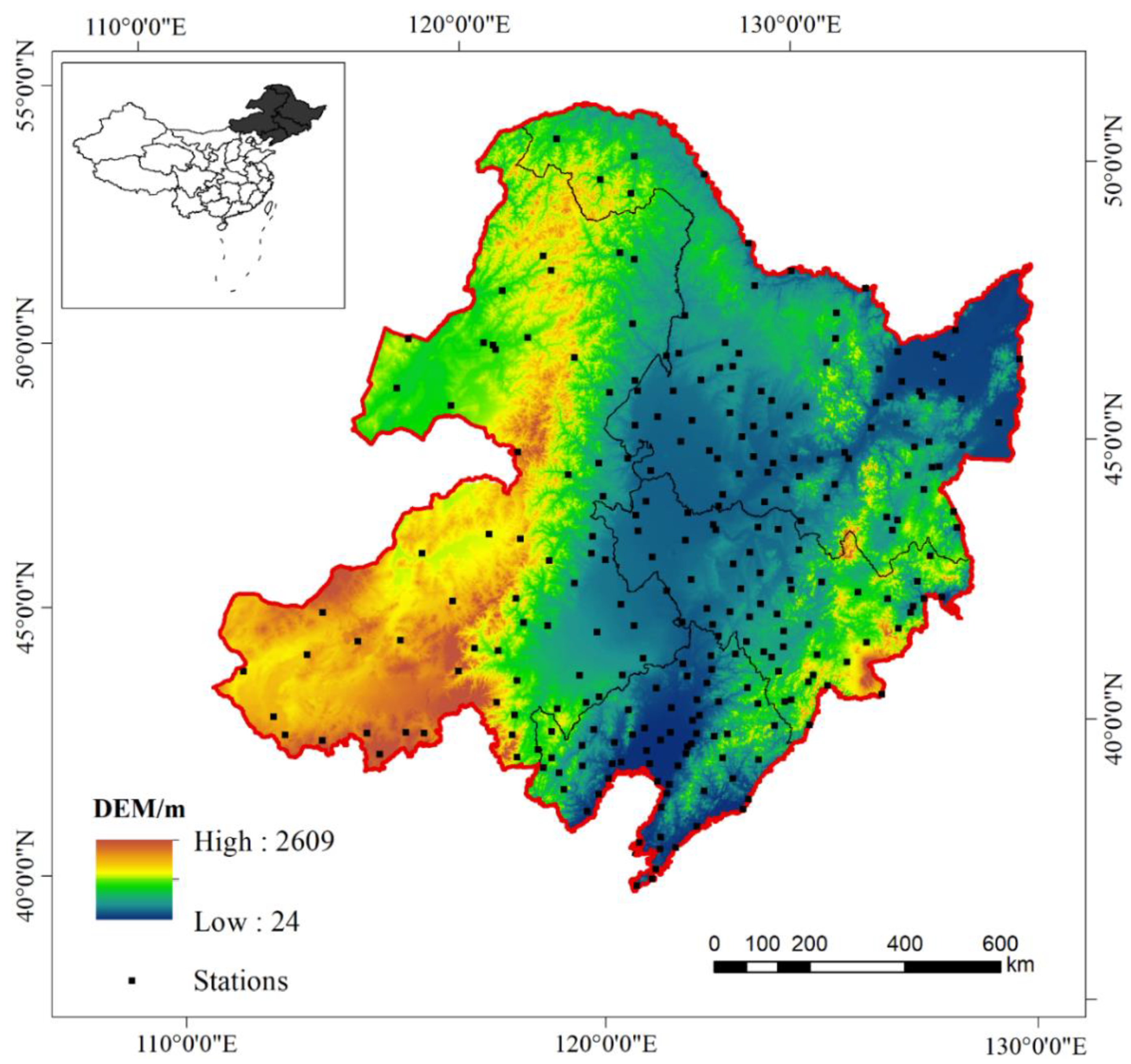
2.1. Study Area

North East China (38°42′N~53°34′N, 117°16′E~135°21′E) is located in the high-latitude region of eastern Eurasia, spanning four provinces, including Heilongjiang, Jilin, Liaoning and the northeastern part of Inner Mongolia (Figure 1), and covers an area of 16.13 × 10⁵ km². North East China belongs to the moderate-temperature and cold-temperate monsoon climate zones, with a mean annual temperature ranging from approximately −4 to 11 °C. The mean annual rainfall decreases from the southeast (1000 mm) to the northwest (300 mm), spanning from the wet zone to the semihumid and semiarid zones [41]. All of these annual averages were derived from weather stations in the study area in 2016. The soil types in North East China are dominated by high-fertility black soil (the average organic content is between approximately 3% and 10%). The vegetation types include cold-temperate coniferous forests distributed in the northern part of the Greater Xing’an Mountains, coniferous and broad-leaved mixed forests in the eastern mountains, and temperate forests and grasslands in the central plains. The main land cover types in the region are forestland, dryland, paddy fields, and grassland, accounting for 41.50%, 27.78%, 3.62%, and 18.53% of the total area, respectively [42]. The study area is centered on the Songnen Plain, and a horseshoe-shaped landform pattern is formed in the east, north, and west. The northern part of the Greater Xing’an Mountains in the northwest includes a series of mountain ranges: Xiaoxing’anling in the north, Daheishan in the middle, Hadaling in Jilin Province, and Zhangguangcailing, Laoyeling, Wandashan, and Changbai in the south. Typical dry-wet differentiation, a unique vegetation distribution, and relatively complete natural geographic regions, combined with seasonal interdecadal features of seasonal precipitation and temperature, are closely related to the occurrence of extreme weather events (such as droughts and floods); thus, North East China has become a hot spot for global climate change and ecological geography research [43].

2.2. Datasets

2.2.1. LST and NDVI

We used the LST and NDVI RS products retrieved from MODIS, which is onboard the Aqua satellite; these products have been widely used to monitor surface, oceanic, and atmospheric conditions [44,45]. Aqua passes over North East China at approximately 01:30 a.m. (descending) and 01:30 p.m. (ascending). In this study, the MODIS products were obtained from National Aeronautics and Space Administration’s (NASA’s) Earth Observing System Data and Information System. The 1-km, 8-day composite LST (day/night) product MYD11A2 and the 1-km 16-day composite NDVI product MYD13A3 were used as inputs in the TVDI model.

2.2.2. Soil Moisture (SM)

The soil moisture data (humidity unit: m³/m³) were mainly derived from the Level-3 products of AMSR-E, SMOS, and AMSR2, with resolutions of 25, 25, and 10 km, respectively. The AMSR-E sensor is mounted on the Aqua satellite, and its orbital parameters are consistent with those of MODIS. Hence, the AMSR-E Level 3 products were included in the analysis for both day (01:30 p.m.) and night (01:30 a.m.) overpasses. The time span was from July 2002 to September 2011, and the data were provided by the Japan Aerospace Exploration Agency (JAXA, http://global.jaxa.jp/projects/sat/gcom_w/index.html). The AMSR-E SM products were retrieved using the vertically and horizontally polarized brightness temperature (Tb) from the C-band (7.3 GHz) and the X-band (10.7 GHz). The AMSR2 instrument is onboard the Global Change Observation Mission–Water 1 (GCOM-W1) satellite, which was launched by JAXA in May 2012 and measures C-band and X-band emissions with overpass times of 01:30 a.m. and 01:30 p.m. [46]. As a successor to AMSR-E, AMSR2 provides near-real-time passive microwave observations [47]. The AMSR2 Level 3 SM data were provided by JAXA’s GCOM website (http://suzaku.eorc.jaxa.jp/).

The European Space Agency’s (ESA’s) SMOS mission, which was launched in 2009 as part of the Living Planet Programme, was used to study the L-band (1.4 GHz) emissions. The transit times of the ascending and descending orbits are at approximately 06:00 a.m. and 06:00 p.m., respectively, in local time (~3 days), and the study period spanned from October 2011 to June 2012. While the original resolution of the SMOS SM data is 35 to 55 km, the Level 3 products were provided on the Equal Area Scalable Earth (EASE) grid, with a 25-km sampling interval [48]. The data were acquired from ESA’s official website (https://earth.esa.int/). The monthly 25-km resolution SMOS Level-3 product integrates the averages of daytime and nighttime data but does not include individual values for day and night. To make the products consistent, the AMSR-E, AMSR2, and SMOS products were corrected with the time series reconstruction method.

2.2.3. Meteorological Data

In situ SM records were collected from 24-h field stations in North East China from the Soil Moisture on the Growth and Development of Crops in China dataset (http://data.cma.cn/site/index.html, last access: 28 February 2019) provided by the China Meteorological Science Data Service Network (CMSDSN). The in situ SM data were compared with the results of the downscaled SM calculation, and weather anomalies and nonrepresentative data were excluded (Figure 1). Ground SM data were measured at approximately 1:30 p.m. and 1:30 a.m. (local solar time), corresponding to the satellite overpass time. These data were used and compared with the corresponding downscaled daytime and nighttime SM data. The ground-based SM measurements were matched with the grid points of the downscaled SM data using the nearest neighbor approach. In this study, the verification work was carried out on a monthly scale, so the monthly ground station aggregate data were averaged from the daily meteorological site data that were selected.

3. Methods

A summary of the downscaling method is shown in Figure 2, and additional details are described in the following sections.

3.1. Calculation of the TVDI

Theoretically, the temperature will decrease by 6 °C for every 1-km increase in elevation [49], and the elevation difference between the highest and lowest areas in North East China is greater than 2 km. Therefore, we need to correct the MODIS surface temperature products to reduce the impact of elevation on the surface temperature inversion before calculating the TVDI:

T_m = T_s + a * h

(1)

where Tm is the LST after topographic correction, Ts is the surface temperature before topographic correction, and h is the elevation value at the LST pixel. The temperature variables are in °C. The variable a is the average influence coefficient of elevation on the LST inversion process (the common value is 6 °C/km).

In practice, due to weather conditions, there are some missing deviations in some time series data; to compensate for data errors caused by weather conditions, a Savitzky-Golay (S-G) filter timing reconstruction method is applied in this study to improve the quality of the data. The formula for processing the data via S-G filtering is as follows:

$$Y_j^{\ast }={\displaystyle \sum _{i=-m}^{i=m}\frac{C_i{Y}_{j+1}}{N}}$$

(2)

where Y_j^* is the filtered reconstructed data, Y_j+1 is the original time series data, m is the size of the moving filter window, C_i is the fitting coefficient of the S-G filter polynomial, that is, the i-th weight index starting from the filter header of each value, and N is the length of the filter processing data.

The TVDI values were calculated as follows [47]:

TVDI = T_m − T_smin/(T_smax − T_smin)

(3)

where TVDI is the temperature-vegetation dryness index, Tm represents the LST after topographic correction, T_smax is the highest surface temperature on the dry edge corresponding to the NDVI, and T_smin is the lowest surface temperature on the wet edge corresponding to the NDVI. We can calculate T_smax and T_smin as follows:

T_smax = a₁ + b₁ * NDVI

(4)

T_smin = a₂ + b₂ * NDVI

(5)

where a₁ and b₁ represent the slope and intercept on the “dry edge”, respectively, and a₂ and b₂ represent the slope and intercept on the “wet edge”, respectively. NDVI is the normalized difference vegetation index in the study time series (from 2002 to 2018).

3.2. Time Series Reconstruction of Difference Decomposition (TSRDD) Method

The SMOS Level 3 products used in this study are monthly averages of the daytime and nighttime values, and the SMOS and AMSR series satellites have different descending and ascending times. To ensure data consistency and integrity, the time series reconstruction with difference decomposition (TSRDD) method is developed according to the time series principles to capture long-term daytime and nighttime SM series datasets at different times. The TSRDD method includes a consistency correction and generates the daytime and nighttime data from the SMOS series data, thereby obtaining a long-term, high-precision SM dataset that ensures consistency among the multisensor SM data at different times.

Ẑ(x, j) _day = Ẑ(x, j)_average + ΔF_j

(6)

Ẑ(x, j) _night = Ẑ(x, j)_average − ΔF_j

(7)

$$\Delta F_j=\frac{{{\displaystyle \sum }}_{i=1}^{\frac{w}{2}}\left(F_{dayi}-F_{nighti}\right)+{{\displaystyle \sum }}_{i=1+\frac{w}{2}}^w\left(F_{dayi}-F_{nighti}\right)}{w-1}$$

(8)

where Ẑ(x,j)_day is the reconstructed daytime SM in month j of year x and Ẑ(x,j)_night is the reconstructed nighttime SM in month j of year x. $\Delta F_j$ represents the difference between daytime and nighttime (day minus night) in month j. Ẑ(x, j)_average is the average value in month j of year x, and w is the selected year window size.

3.3. Spatial Fusion Downscaling Model (SFDM) of SM

The TVDI is significantly negatively correlated with SM, as shown in previous studies [14]. According to this correlation, the high-resolution TVDI is used to perform the pixel-by-pixel weighting of low-resolution SM data. Then, the weight is used to divide the low spatial resolution SM product into high-spatial-resolution SM products, and the downscaling relationship is as follows:

$$S{M}_i=S{M}_k\times \frac{1-TVD{I}_i}{1-TVD{I}_{average}}$$

(9)

where SM_i is the SM value for a pixel after downscaling and SM_k represents the low-resolution SM data input. TVDI_i is the TVDI value for a pixel that corresponds to the downscaled SM. TVDI_average is the average of all the TVDI values corresponding to the SM_k pixels.

3.4. The Calculation of the Trend of the Variation in SM

To analyze the change (increase or decrease) in the spatial pattern and the amplitude of the SM from 2002 to 2018, the variation rates and correlation coefficient were calculated based on the SM values of the pixels over the study area as follows:

$$Slope=\frac{n{{\displaystyle \sum }}_{i=1}^n\left(i\times p_i\right)\times \left({{\displaystyle \sum }}_{i=1}^{n}i\right)\times \left({{\displaystyle \sum }}_{i=1}^n{p}_i\right)}{\left(n\times {{\displaystyle \sum }}_i^n{i}^2\right)-{\left({{\displaystyle \sum }}_{i=1}^{n}i\right)}^2}$$

(10)

$$R=\frac{n{{\displaystyle \sum }}_{i=1}^n\left(i\times p_i\right)-\left({{\displaystyle \sum }}_{i=1}^{n}i\right)\times \left({{\displaystyle \sum }}_{i=1}^n{p}_i\right)}{\sqrt{\left(n{{\displaystyle \sum }}_i^n{i}^2\right)-{\left({{\displaystyle \sum }}_{i=1}^{n}i\right)}^2}\times \sqrt{\left(n{{\displaystyle \sum }}_i^n{p}_i{}^2\right)-{\left({{\displaystyle \sum }}_{i=1}^n{p}_i\right)}^2}}$$

(11)

where Slope is the trend in the SM during the study time series, i represents the number of years, n represents the number of time series, and p_i represents the SM value of the i-th year. If Slope is positive, then the SM has increased from the previous time point. If Slope is negative, then the SM has decreased from the previous time point. If Slope = 0, then there is no change from the previous time point. R is the correlation coefficient between the change in the SM and the time in the time series. The larger the absolute value of R is, the stronger the correlation.

3.5. Soil Moisture Anomaly (SMA) Index

The soil moisture anomaly (SMA) index is used to describe dramatic changes in the SM in the study region (too low or too high), and the SMA index can be derived from the following formula [27]:

SMA_{i(x, y)} = (SM_{i(x, y)} − SM_{min(x, y)})/(SM_{max(x, y)} − SM_{min(x, y)}) × 100%

(12)

where SMA_{i(x, y)} is the SMA index of pixel (x, y) at time i, SM_{i(x, y)} is the SM value of pixel (x, y) at time i, SM_{max(x, y)} is the maximum SM value of pixel (x, y) during the study period, SM_{min(x, y)} is the maximum SM value of pixel (x, y) during the study period, and SM_{average(x, y)} is the average SM value of pixel (x, y) during the study period.

3.6. Drought and Flood Degree

To characterize the spatiotemporal distribution of drought and waterlogging over the 198 months from 2002 to 2018 (excluding January to June 2002), the SMA index was divided into seven grades based on the literature concerning drought and waterlogging classification standards: slight waterlogging (SLW), moderate waterlogging (MOW), normal (no disasters), severe waterlogging (SEW), slight drought (SLD), moderate drought (MOD), and severe drought (SED), as shown in

Table 1. Definitions of disaster levels.

Disaster Type	SMA Values	Description
Slight waterlogging	90%–100%	The soil is very damp/extremely wet, and the color is dark
Moderate waterlogging	80%–90%	The soil is damp and brown, and there is water in low-lying places
Severe waterlogging	70%–80%	The soil is moist, and the color is brown
Normal	40%–70%	The soil moisture is within the normal range
Slight drought	30%–40%	Less soil moisture, and there is a risk for drought
Moderate drought	20%–30%	The soil is semidry
Severe drought	10%–20%	The soil is dry, and drought will occur

.

4. Results

4.1. Verification

4.1.1. TSRDD Verification

To ensure the consistency of the data between different sensors and obtain the SMOS daytime and nighttime data, the most suitable timing window is selected. The SM value is normally distributed in the study area, which satisfies the basic conditions for the correlation analysis between the simulated, corrected, and original values. The relationship between the corrected variables and explanatory variables (original value) varies significantly for different window sizes (w). The regression coefficients (root mean squared error (RMSE), mean absolute error (MAE), and R²) of the TSRDD are presented in

Table 2. The mean RMSE, MAE, and R² values between the corrected values of variable z and explanatory variables (original value) in the time series reconstruction of the difference decomposition (TSRDD) for different window sizes.

	Day			Night
w 1	RMSE (m3/m3)	MAE (m3/m3)	R2	RMSE (m3/m3)	MAE (m3/m3)	R2
3	2.13	1.51	0.92	2.07	1.56	0.95
5	2.11	1.46	0.96	2.12	1.54	0.95
7	2.10	1.54	0.96	2.14	1.62	0.96
9	2.15	1.54	0.92	2.05	1.51	0.96
11	2.16	1.61	0.95	2.12	1.53	0.96
13	2.25	1.61	0.94	2.14	1.59	0.91
15	2.16	1.49	0.96	2.12	1.54	0.95
17	2.25	1.56	0.96	2.07	1.56	0.95
Average	2.16	1.54	0.95	2.10	1.56	0.95

¹ W is the window size for the selected year from formula (8).

.

For daytime, the indexes are best matched when w is 5: the RMSE (m³/m³), MAE (m³/m³), and R² are 2.11, 1.46, and 0.96, respectively. For nighttime, the indexes are best matched when w is 3: the RMSE (m³/m³), MAE (m³/m³), and R² are 2.07, 1.56, and 0.95, respectively. Therefore, these two windows are used to decompose the SM data from the SMOS daytime and nighttime data.

4.1.2. Downscaled SM Verification

To quantitatively evaluate the performance of daytime and nighttime downscaling, considering the effects of weather factors, we compared the downscaled passive microwave SM values (at the 1-km scale) with meteorological in situ SM observations scattered throughout the North East China area for daytime and nighttime, and the R², RMSE, and bias values were used for the comparison. The results showed that the downscaled and in situ observed SM were strongly correlated, with mean R² values of 0.61 and 0.73 for daytime and nighttime, respectively (Figure 3). The mean RMSE and bias values were 0.10 m³/m³ and 0.07 m³/m³ for daytime and 0.12 m³/m³ and 0.06 m³/m³ for nighttime, respectively. The results indicated a significantly high correlation between the downscaled passive microwave and in situ measured SM data during the daytime (Figure 3a) and nighttime (Figure 3b).

Figure 3 and Figure 4 display the accuracy analysis and show significant spatiotemporal differences between day and night. First, the R² values of the nighttime observations were slightly higher than those of the daytime observations. Second, the points were more aggregated at night than during the day. One possible reason for the increased nighttime accuracy may be the difference in the time lag between the downscaled SM and in situ observations. Similar results were reported for LST and measured temperature [50]. The accuracy analysis also presented a certain spatial differentiation: The RMSE was high along rivers and coasts, as well as in some mountainous areas (>0.3), in the daytime, and the RMSE was low (<0.1) in the plain regions. Moreover, the spatial differentiation characteristics at night were less obvious than those during the day (except for several stations along the boundary).

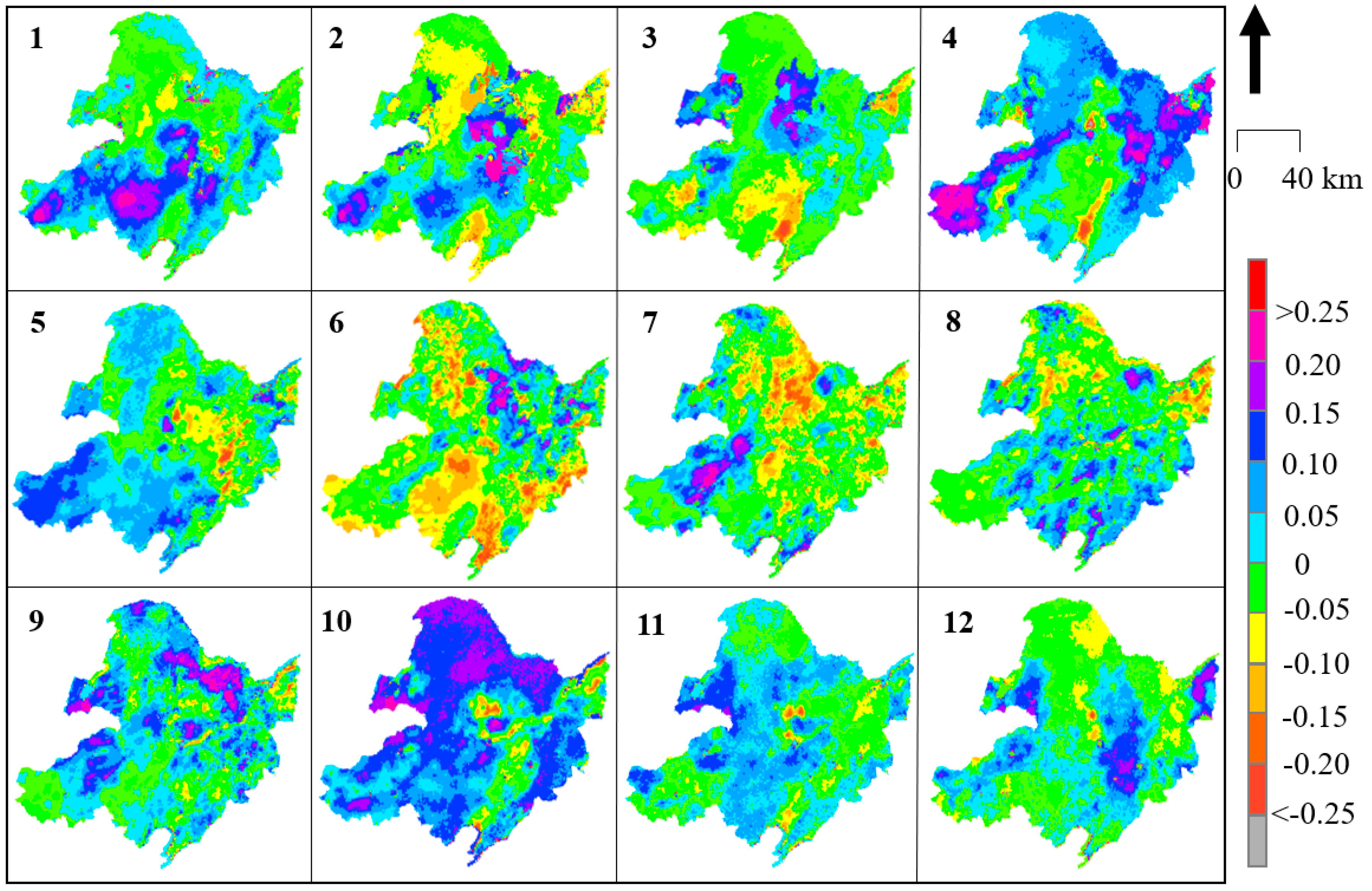
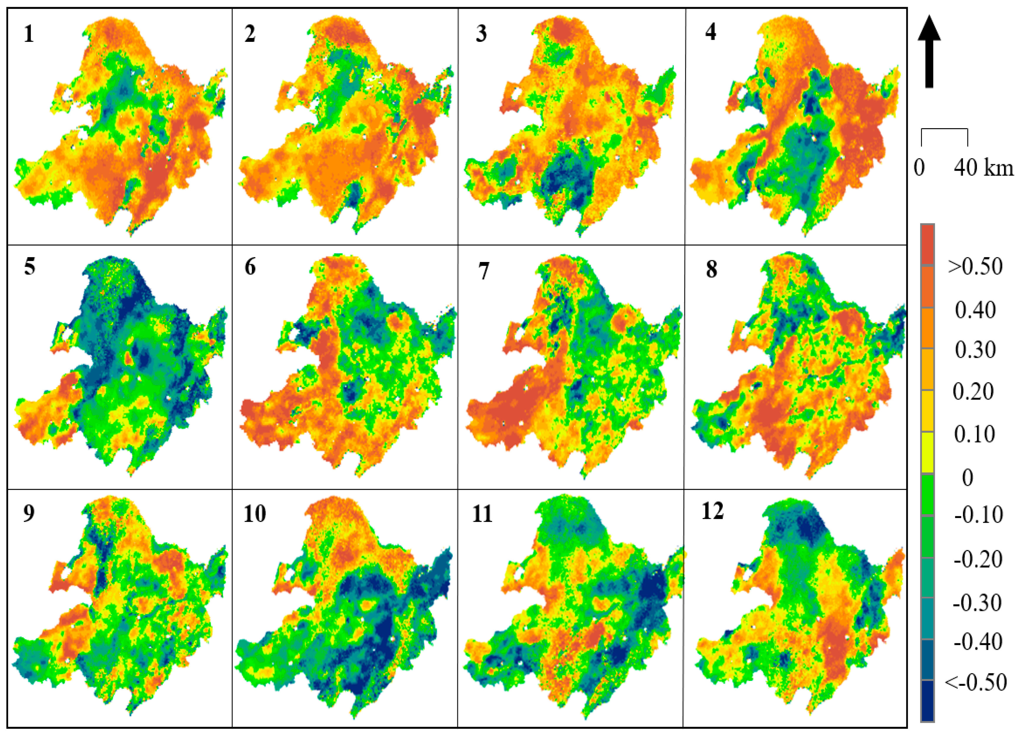
4.2. Spatiotemporal Variation in the SM

The downscaled SM showed significant spatiotemporal variations spanning different seasons and regions. We aggregated the downscaled SM by month for four regions in North East China (Figure 5). The mean monthly daytime SM in the four regions ranged from approximately 0.03 m³/m³ (February in Heilongjiang) to 0.16 m³/m³ (June in Heilongjiang). Similarly, the mean monthly nighttime SM ranged from 0.03 m³/m³ (February in Heilongjiang) to 0.20 m³/m³ (June in Heilongjiang). The downscaled SM also showed significant temporal patterns. First, there were apparent seasonal variations in the SM values, with high values in summer and low values in winter (Figure 5). There was an east-west distribution pattern, and in the eastern region, there was a valley in July (summer). One possible reason for the “bimodal” distribution in the eastern region could be that the distance between land and sea and the sinking airflow from the Greater Xing’an Mountains reduced precipitation in the coastal areas in July.

To obtain the spatiotemporal rate of change in the downscaled SM in North East China in detail, formulas (9) and (10) were utilized to calculate the monthly changes using every pixel from 2002 to 2018 (Figure 6 and Figure 7 represent the Slope values for daytime and nighttime, respectively; Figure 8 and Figure 9 represent the R values for daytime and nighttime, respectively). As shown in Figure 6, the SM in the North East China region significantly increased over the past 17 years, with obvious monthly differences. The SM distribution in North East China was more stable at night than during the day. The most significant changes in SM during the day occurred in spring (April) and autumn (October), and the two trends were consistent. This “correspondence phenomenon” is thought to be related to the interaction between vegetation and climate (this trend is present during both the day and night). The SM variation in North East China exhibited obvious seasonality. In spring (March, April, and May), the southwestern region (particularly in the Inner Mongolia area) suffered from the highest increasing trend, with an increasing Slope of more than 0.3 (R > 0.20) that extended over 35.7% of the Xiaoxing’anling area. The increase was also greater than 0.3 (R > 0.25) in the Songnen Plain and the Sanjiang Plain in April (in the daytime). The variation in summer (June, July and August) was relatively uniform, and the Slope value of the change was within 0.2 (in the daytime and nighttime). Almost everywhere across North East China, except for a few mountain areas, the Slope value decreased, including in the southern Greater Xing’an Mountains (less than −0.2), while the Slope value south of Xiaoxing’anling increased (greater than 0.2), and the Slope was slightly higher in summer than in other seasons. There were dramatic changes in the spatial patterns of the SM values during autumn (September, October, and November). The SM values increased in the northwest (Slope > 0.20, R > 0.20) and decreased in the southeast (Slope < −0.20, R < −0.10). In winter (November, December, and January), the southern region centered at the Horqin Sandy Land exhibited an increase in Slope (>0.4), and the opposite was observed in summer (May: Slope < −0.3).

Overall, the consistencies of the daytime and nighttime changes in autumn and winter were better than those in spring and summer, and the consistency in the western region (northeastern Inner Mongolia) was better than that in the eastern region (Liaoning, Jilin, Heilongjiang). One possible reason for this phenomenon is that the vegetation density is high and complex in the east, the river network is dense, and the soil evapotranspiration changes greatly between day and night, so there will be large differences between daytime and nighttime.

4.3. Spatiotemporal Variations in SMA

Although the monthly variations in Slope and the correlation coefficient R show the spatial trends of SM (Figure 6, Figure 7, Figure 8 and Figure 9), some annual abnormalities need to be further analyzed. As shown in Figure 10 and Figure 11, the SMAs are mapped to investigate the spatial distribution of soil water anomalies during the daytime and nighttime over 17 years. The large-scale severe drought phase mainly occurred in three periods, 2008, 2015, and 2018. In 2008, a large-scale rain and snow disaster occurred in southern China, and the Wenchuan earthquake caused intense crustal movement. According to the SMA analysis, SLD conditions were mainly concentrated in the northern part of Inner Mongolia and the Hulunbeier Plateau in the west of Heilongjiang (daytime), and the area with SED conditions accounted for more than 80% of the total study area (average of daytime and nighttime). In this survey, the area with SED conditions accounted for 75% in 2015, that is, more than 3/4 of the total drought and drought risk area. In 2015, a large-scale drought occurred in the northeastern region. The drought in 2018 was consistent with the agricultural drought in the spring and summer (daytime and nighttime means). The large-scale and severe waterlogging phases mainly occurred in two periods, 2003 and 2014. The waterlogging situation in 2003 did not exhibit a wide spatial distribution, but it still caused abnormal changes within Bohai Bay (the affected area exceeded 4.82 × 104 km²). The SMA value of some regions increased in 2014, such as the Changbai Mountain area, but the flood trends became more obvious. Combined with a large amount of snowfall in the winter of 2013, there were some impacts on the accuracy of SM extraction in this area. Additionally, the daytime SMA exhibited increased variation, especially in the mountain areas, and this variation was greater than that in the nighttime SMA areas. The radiation is greater and active vegetation evapotranspiration and soil water evaporation are higher during the day than at night; however, these values also exhibit greater changes during the day than at night.

Snow (ice) coverage and low temperatures are mutually influential processes in winter. Snow accumulation leads to an increase in surface reflectivity, which reduces the radiant energy absorbed by the surface and decreases the temperature. The decreased temperature will reduce the speed of snow melting. Therefore, the large amount of snowfall in winter in recent years can be considered one of the main causes of spring disasters in North East China. Second, the increase in the amount of spring rainfall further increases the severity of spring floods, resulting in increased SM on the surface, the formation of stagnant water in low-lying areas, and delays in spring plowing (especially in the Songnen Plain). Other studies have shown that Mongolia’s high-pressure systems and subtropical high-pressure belts, the main wind circulation of the westerly belt and the southwest water vapor transmission rate have all been weakened. We have greatly improved the spatiotemporal monitoring of SM, and the trends and disaster distributions based on the downscaled SM could provide references for the creation of climate change policies and monitoring of extreme weather.

5. Discussion and Conclusions

In this paper, an SFDM is constructed using passive microwave SM data and MODIS LST/NDVI data, and a time series reconstruction with the TSRDD method is used to ensure the continuity and consistency of long-term SM data sequences. By comparing the relative precision of different time series windows, the optimal window is selected to decompose the SM data with coarse spatial resolution into a high-resolution, continuous, monthly daytime and nighttime SM dataset (spanning 2002~2018, ~1 km). The in situ validation analysis resulted in R² values of 0.61 and 0.73 for daytime and nighttime, respectively, and the average RMSE and bias values were 0.10 m³/m³ and 0.07 m³/m³ for daytime and 0.12 m³/m³ and 0.06 m³/m³ for nighttime, respectively. These results demonstrated that the method for downscaling the SM to 1-km resolution could reliably capture the variability in the daytime and nighttime soil water contents in North East China. We calculated the spatiotemporal distribution of the SM trends and statistically investigated the characteristics and patterns of droughts and floods in various regions of North East China with the SMA index. In the next step of this study, the response relationship between global meteorological phenomena and local disasters need to further quantitatively explored.

References

1. Global Climate Observing System (GCOS). Systematic Observation Requirements for Satellite-Based Products for Climate, 2011 Update, Supplemental Details to the Satellite-Based Component of the Implementation Plan for the Global Observing System for Climate in Support of the UNFCCC (2010 Update). 2011. p. 138. Available online: http://www.wmo.int/pages/prog/gcos/Publications/gcos-154.pdf (accessed on 13 November 2012).
2. Kerr, Y.H.; Waldteufel, P.; Richaume, P.; Wigneron, J.P.; Ferrazzoli, P.; Mahmoodi, A.; Al Bitar, A.; Cabot, F.; Gruhier, C.; Juglea, S.E.; et al. The SMOS soil moisture retrieval algorithm. IEEE Trans. Geosci. Remote Sens. 2012, 50, 1384–1403. [Google Scholar] [CrossRef]
3. Bindlish, R.; Crow, W.; Jackson, T. Role of passive microwave remote sensing in improving flood forecasts. IEEE Geosci. Remote Sens. Lett. 2009, 6, 112–116. [Google Scholar] [CrossRef]
4. Gao, Z.; Wang, Q.; Cao, X.; Gao, W. The responses of vegetation water content (EWT) and assessment of drought monitoring along a coastal region using remote sensing. GISci. Remote Sens. 2014, 51, 1–16. [Google Scholar] [CrossRef]
5. Elbialy, S.; Mahmoud, A.; Pradhan, B.; Buchroithner, M. Application of spaceborne synthetic aperture radar data for extraction of soil moisture and its use in hydrological modelling at Gottleuba Catchment, Saxony, Germany. J. Flood Risk Manag. 2014, 7, 159–175. [Google Scholar] [CrossRef]
6. Peng, J.; Loew, A.; Zhang, S.; Wang, J. Spatial downscaling of global satellite soil moisture data using temperature vegetation dryness index. IEEE Trans. Geosci. Remote Sens. 2016, 1, 558–566. [Google Scholar] [CrossRef]
7. Van Loon, A.F.; Gleeson, T.; Clark, J.; Van Dijk, A.I.J.M.; Stahl, K.; Hannaford, J.; Di Baldassarre, G.; Teuling, A.J.; Tallaksen, L.M.; Uijlenhoet, R.; et al. Drought in the anthropocene. Nat. Geosci. 2016, 9, 89–91. [Google Scholar] [CrossRef]
8. Lakshmi, V. Remote sensing of soil moisture. ISRN Soil Sci. 2013, 33. [Google Scholar] [CrossRef]
9. Mohanty, B.P.; Cosh, M.H.; Lakshmi, V.; Montzka, C. Soil moisture remote sensing: State-of-the-science. Vadose Zone J. 2017, 16. [Google Scholar] [CrossRef]
10. Kogan, F.N. Remote sensing of weather impacts on vegetation in nonhomogeneous areas. Int. J. Remote Sens. 1990, 11, 1405–1419. [Google Scholar] [CrossRef]
11. Zhang, D.; Zhou, G. Estimation of Soil Moisture from Optical and Thermal Remote Sensing: A Review. Sensors 2016, 16, 1308. [Google Scholar] [CrossRef]
12. Kogan, F.N. Application of vegetation index and brightness temperature for drought detection. Adv. Space Res. 1995, 15, 91–100. [Google Scholar] [CrossRef]
13. Carlson, T.N.; Gillies, R.R.; Perry, E.M. A method to make use of thermal infrared temperature and NDVI measurements to infer surface soil water. Remote Sens. Rev. 1994, 9, 161–173. [Google Scholar] [CrossRef]
14. Sandholt, I.; Rasmussen, K.; Andersen, J. A simple interpretation of the surface temperature/vegetation index space for assessment of surface moisture status. Remote Sens. Environ. 2002, 79, 213–224. [Google Scholar] [CrossRef]
15. Chauhan, N.S.; Miller, S.; Ardanuy, P. Spaceborne soil moisture estimation at high resolution: A microwave–optical/IR synergistic approach. Int. J. Remote Sens. 2003, 24, 4599–4622. [Google Scholar] [CrossRef]
16. Owe, M.; De Jeu, R.; Holmes, T. Multisensor historical climatology of satellite-derived global land surface moisture. J. Geophys. Res. 2008, 113, F01002. [Google Scholar] [CrossRef]
17. Shi, J.C.; Du, Y.; Du, J.Y.; Jiang, L.M.; Chai, L.N.; Mao, K.B.; Xu, P.; Ni, W.J.; Xiong, C.; Liu, Q.; et al. Progresses on microwave remote sensing of land surface parameters. Sci. China Earth Sci. 2012, 55, 1052–1078. [Google Scholar] [CrossRef]
18. Fang, B.; Lakshmi, V.; Bindlish, R.; Thomas, J.J. AMSR2 soil moisture downscaling using temperature and vegetation data. Remote Sens. 2018, 10, 1575. [Google Scholar] [CrossRef]
19. Sridhar, V.; Jaksa, W.T.A.; Fang, B.; Lakshmi, V.; Hubbard, K.G.; Jin, X. Evaluating bias–corrected AMSR–E soil moisture using in situ observations and model estimates. Vadose Zone J. 2013, 12, 1712–1717. [Google Scholar] [CrossRef]
20. Minet, J.; Bogaert, P.; Vanclooster, M.; Lambot, S. Validation of ground penetrating radar full–waveform inversion for field scale soil moisture mapping. J. Hydrol. 2012, 424, 112–123. [Google Scholar] [CrossRef]
21. Njoku, E.G.; Entekhabi, D. Passive microwave remote sensing of soil moisture. J. Hydrol. 1996, 184, 101–129. [Google Scholar] [CrossRef]
22. Mao, K.; Tang, H.J.; Zhang, L.X.; Li, M.C.; Guo, Y.; Zhao, D.Z. A method for retrieving soil moisture in Tibet region by utilizing microwave index from TRMM/TMI data. Int. J. Remote Sens. 2008, 29, 2905–2925. [Google Scholar] [CrossRef]
23. Wagner, W.; Sabel, D.; Doubkova, M.; Bartsch, A.; Pathe, C. The potential of Sentinel-1 for monitoring soil moisture with a high spatial resolution at global scale. In Proceedings of the Earth Observation and Water Cycle Science Symposium, Frascati, Italy, 18–20 November 2009. [Google Scholar]
24. Shen, X.; Yang, H.; Qiming, Q.; Jeffery, B.; Mao, K. A semi-physical microwave surface emission model for soil moisture retrieval. IEEE Trans. Geosci. Remote Sens. 2015, 53, 4079–4090. [Google Scholar] [CrossRef]
25. Shen, X.; Hong, Y.; Qin, Q.; Yuan, W. Bare surface soil moisture estimation using double-angle and dual-polarization L-band radar data. IEEE Trans. Geosci. Remote Sens. 2013, 51, 3931–3942. [Google Scholar] [CrossRef]
26. Kerr, Y.H.; Jacquette, E.; Al Bitar, A.; Cabot, F.; Mialon, A.; Richaume, P.; Quesney, A.; Berthon, L.; Wigneron, J. CATDS SMOS L3 Soil Moisture Retrieval Processor: Algorithm Theoretical Baseline Document (ATBD); CESBIO: Toulouse, France, 2013. [Google Scholar]
27. Champagne, C.; Mcnairn, H.; Berg, A.A. Monitoring agricultural soil moisture extremes in Canada using passive microwave remote sensing. Remote Sens. Environ. 2011, 115, 2434–2444. [Google Scholar] [CrossRef]
28. Peng, J.; Niesel, J.; Loew, A. Evaluation of soil moisture downscaling using a simple thermal based proxy—The remedhus network (Spain) example. Hydrol. Earth Syst. Sci. 2015, 12, 8505–8551. [Google Scholar] [CrossRef]
29. Peng, J.; Loew, A.; Merlin, O.; Verhoest, N. A review of methods for downscaling remotely sensed soil moisture. Rev. Geophys. 2017, 55, 341–366. [Google Scholar] [CrossRef]
30. Narayan, U.; Lakshmi, V.; Jackson, T.J. High-resolution change estimation of soil moisture using L-band radiometer and Rada observations made during the SMEX02 experiments. IEEE Trans. Geosci. Remote Sens. 2006, 44, 1545–1555. [Google Scholar] [CrossRef]
31. Njoku, E.G.; Wilson, W.J.; Yueh, S.H.; Dinardo, S.J.; Li, F.K.; Jackson, T.J.; Lakshmi, V.; Bolten, J. Observations of soil moisture using a passive and active low-frequency microwave airborne sensor during SGP99. IEEE Trans. Geosci. Remote Sens. 2002, 40, 2659–2673. [Google Scholar] [CrossRef]
32. Chauhan, N.S. Soil moisture estimation under a vegetation cover: Combined active passive microwave remote sensing approach. Int. J. Remote Sens. 1997, 18, 1079–1097. [Google Scholar] [CrossRef]
33. Lee, K.H.; Anagnostou, E.N. A combined passive/active microwave remote sensing approach for surface variable retrieval using Tropical Rainfall Measuring Mission observations. Remote Sens. Environ. 2004, 92, 112–125. [Google Scholar] [CrossRef]
34. Choi, M.; Hur, Y. A microwave-optical/infrared disaggregation for improving spatial representation of soil moisture using AMSR-E and MODIS products. Remote Sens. Environ. 2012, 124, 259–269. [Google Scholar] [CrossRef]
35. Song, C.; Jia, L.; Menenti, M. Retrieving high-resolution surface soil moisture by downscaling AMSR-E brightness temperature using MODIS LST and NDVI data. IEEE J. Sel. Top. Appl. Earth Obs. Remote Sens. 2014, 7, 935–942. [Google Scholar] [CrossRef]
36. Merlin, O.; Al Bitar, A.; Walker, J.P.; Kerr, Y. An improved algorithm for disaggregating microwave–derived soil moisture based on red, near–infrared and thermal–infrared data. Remote Sens. Environ. 2010, 114, 2305–2316. [Google Scholar] [CrossRef]
37. Im, J.; Park, S.; Rhee, J.; Baik, J.; Choi, M. Downscaling of AMSR-E soil moisture with MODIS products using machine learning approaches. Environ. Earth Sci. 2016, 75, 1120. [Google Scholar] [CrossRef]
38. Carlson, T. An overview of the “Triangle Method” for estimating surface evapotranspiration and soil moisture from satellite imagery. Sensors 2007, 7, 1612–1629. [Google Scholar] [CrossRef]
39. Ray, R.L.; Jacobs, J.M.; Cosh, M.H. Landslide susceptibility mapping using downscaled AMSR-E soil moisture: A case study from Cleveland Corral, California, US. Remote Sens. Environ. 2010, 114, 2624–2636. [Google Scholar] [CrossRef]
40. Peng, J.; Loew, A.; Zhang, S.; Wang, J.; Niesel, J. Spatial downscaling of satellite soil moisture data using a vegetation temperature condition index. IEEE Trans. Geosci. Remote Sens. 2016, 54, 558–566. [Google Scholar] [CrossRef]
41. Chen, C.; Qian, C.; Deng, A.; Zhang, W. Progressive and active adaptations of cropping system to climate change in Northeast China. Eur. J. Agron. 2012, 38, 94–103. [Google Scholar] [CrossRef]
42. Liu, Z.; Yang, X.; Chen, F.; Wang, E. The effects of past climate change on the northern limits of maize planting in Northeast China. Clim. Chang. 2013, 117, 891–902. [Google Scholar] [CrossRef]
43. Deng, X.; Jiang, Q.; Zhan, J.; He, S.; Lin, Y. Simulation on the dynamics of forest area changes in northeast China. J. Geogr. Sci. 2010, 20, 495–509. [Google Scholar] [CrossRef]
44. Wan, Z.; Li, Z.L. A physics–based algorithm for retrieving land–surface emissivity and temperature from EOS/MODIS data. IEEE Trans. Geosci. Remote Sens. 1997, 35, 980–996. [Google Scholar]
45. Parkinson, C.L. Aqua: An Earth-observing satellite mission to examine water and other climate variables. IEEE Trans. Geosci. Remote Sens. 2003, 41, 173–183. [Google Scholar] [CrossRef]
46. Imaoka, K.; Kachi, M.; Fujii, H.; Murakami, H.; Hori, M.; Ono, A.; Igarashi, T.; Nakagawa, K.; Oki, T.; Honda, Y.; et al. Global Change Observation Mission (GCOM) for monitoring carbon, water cycles, and climate change. Proc. IEEE 2010, 98, 717–734. [Google Scholar] [CrossRef]
47. Yee, M.S.; Walker, J.P.; Rüdiger, C.; Parinussa, R.M.; Koike, T.; Kerr, Y.H. A comparison of SMOS and AMSR2 soil moisture using representative sites of the OzNet monitoring network. Remote Sens. Environ. 2017, 195, 297–312. [Google Scholar] [CrossRef]
48. Kerr, Y.H.; Waldteufel, P.; Wigneron, J.P.; Delwart, S.; Cabot, F.; Boutin, J.; Escorihuela, M.J.; Font, J.; Reul, N.; Gruhier, C.; et al. The smos mission: New tool for monitoring key elements of the global water cycle. Proc. IEEE 2010, 98, 666–687. [Google Scholar] [CrossRef]
49. Wee, S.; Park, I.S. Plume Dispersion Characteristics in Various Ambient Air Temperature Gradient Conditions. Numer. Heat Transf. 2009, 56, 807–826. [Google Scholar] [CrossRef]
50. Li, X.; Zhou, Y.; Asrar, G.R.; Zhu, Z. Developing a 1 km resolution daily air temperature dataset for urban and surrounding areas in the conterminous United States. Remote Sens. Environ. 2018, 215, 74–84. [Google Scholar] [CrossRef]
Figure 1. The location and topography of the study area and 262 ground meteorological sites in the study area where data were collected.
Sensors 19 03527 g001
Figure 2. Flow chart of the downscaling process.
Sensors 19 03527 g002
Figure 3. Downscaled soil moisture (SM) (1-km scale) based on the spatial fusion downscaling model (SFDM) versus the in situ SM: (a) daytime; (b) nighttime. The solid line is the trend line.
Sensors 19 03527 g003
Figure 4. Spatial variations in the RMSE for each meteorological station in the study area in the study time series for (a) daytime and (b) nighttime.
Sensors 19 03527 g004
Figure 5. Mean monthly daytime and nighttime downscaled SM from January to December in various parts of North East China (NEC). 1: Liaoning, 2: Jilin, 3: Heilongjiang, 4: northeastern Inner Mongolia.
Sensors 19 03527 g005
Figure 6. Trends in Slope for the mean monthly downscaled daytime SM from 2002 to 2018 in NEC.
Sensors 19 03527 g006
Figure 7. Trends in Slope for the mean monthly downscaled nighttime SM from 2002 to 2018 in NEC.
Sensors 19 03527 g007
Figure 8. Trends in R for the mean monthly downscaled daytime SM from 2002 to 2018 in NEC.
Sensors 19 03527 g008
Figure 9. Trends in R for the mean monthly downscaled nighttime SM from 2002 to 2018 in NEC.
Sensors 19 03527 g009
Figure 10. Spatial distribution of daytime soil moisture anomaly (SMA) in NEC from 2002 to 2018.
Sensors 19 03527 g010
Figure 11. Spatial distribution of the nighttime SMA in NEC from 2002 to 2018.
Sensors 19 03527 g011