Hand Movement Classification Using Burg Reflection Coefficients

 , ,
, ,  and
and
Abstract
1. Introduction
2. Materials and Methods
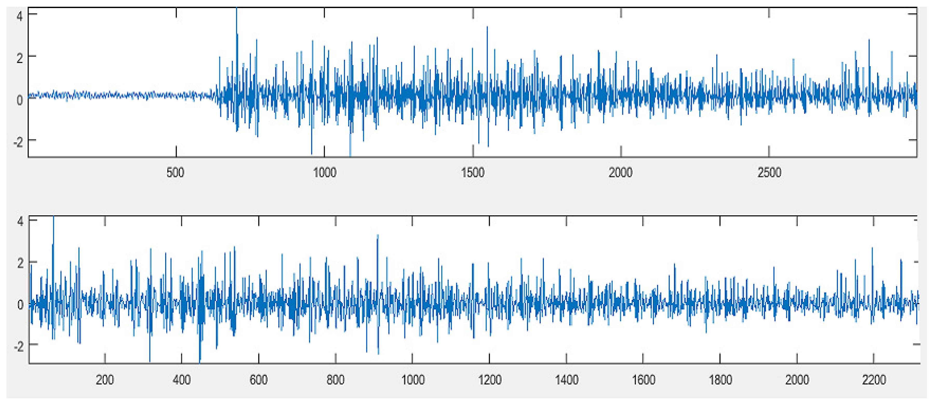
2.1. Data Selection and Preprocessing
2.2. Standard Time Domain Features
2.3. Autoregressive Model Features
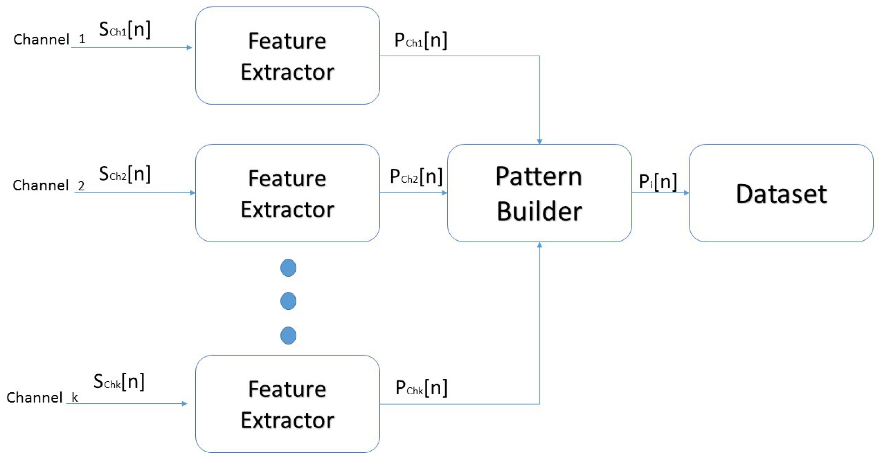
2.4. Dataset Construction
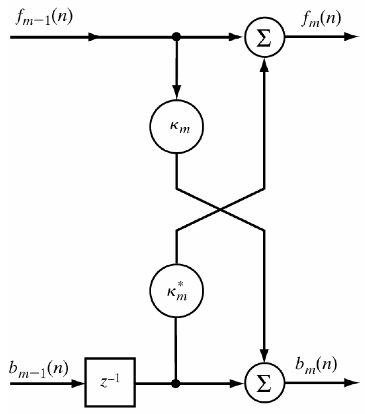
2.5. Proposed Classification Methodology by Applying Burg Reflection Coefficients
2.5.1. Classification Model Training
- Time domain datasets (Equations (1)–(11)): TD= [IEMG MAV SSI VAR RMS WL WAMP SSC ZC MYOP]
- Burg autoregressive coefficients (Equation (17)): Arb = [Arb Arb … Arb]
- Reflection coefficients: K = [K K … K]
2.5.2. Features Selection and Reduction Methods
3. Results
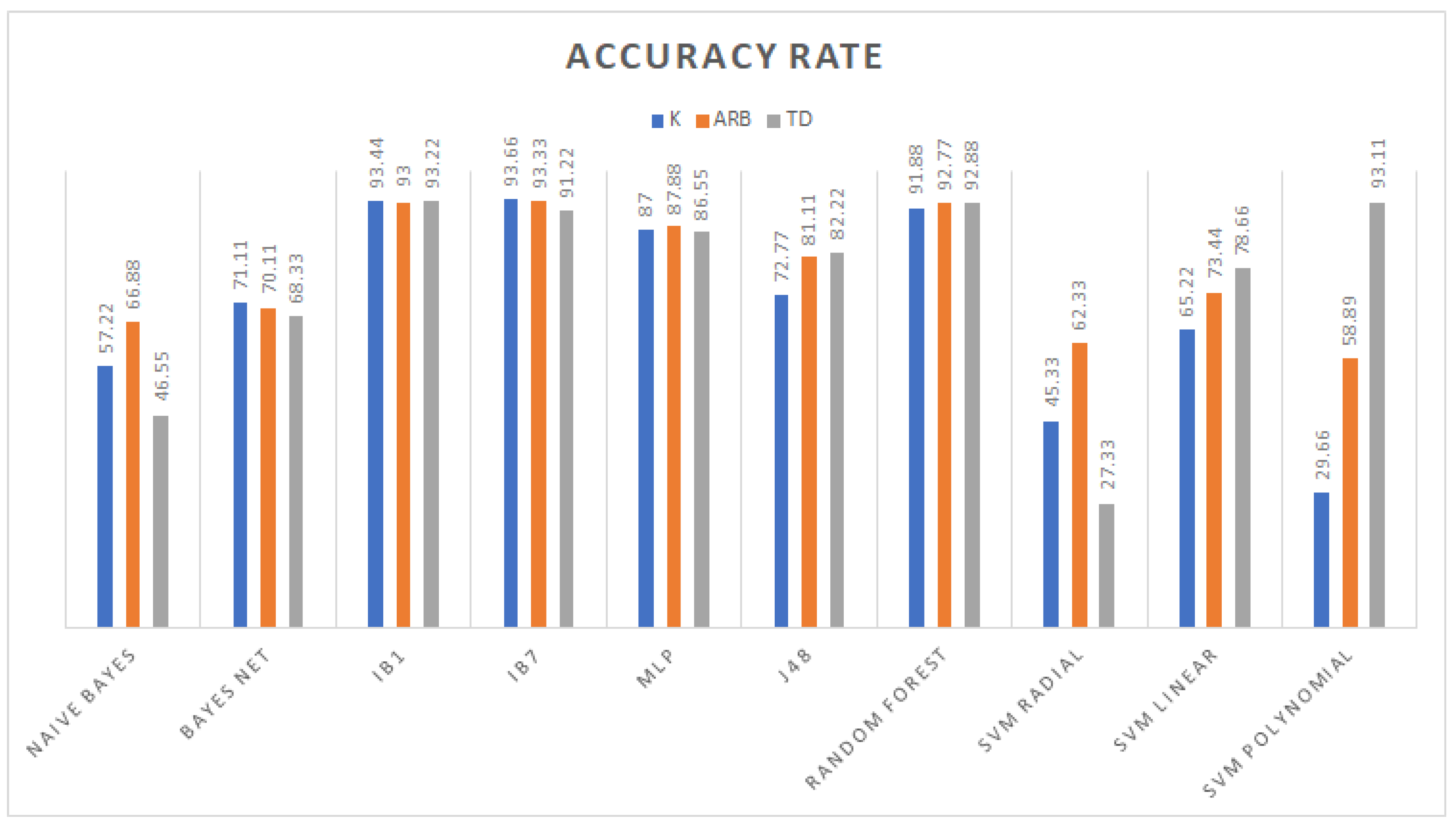
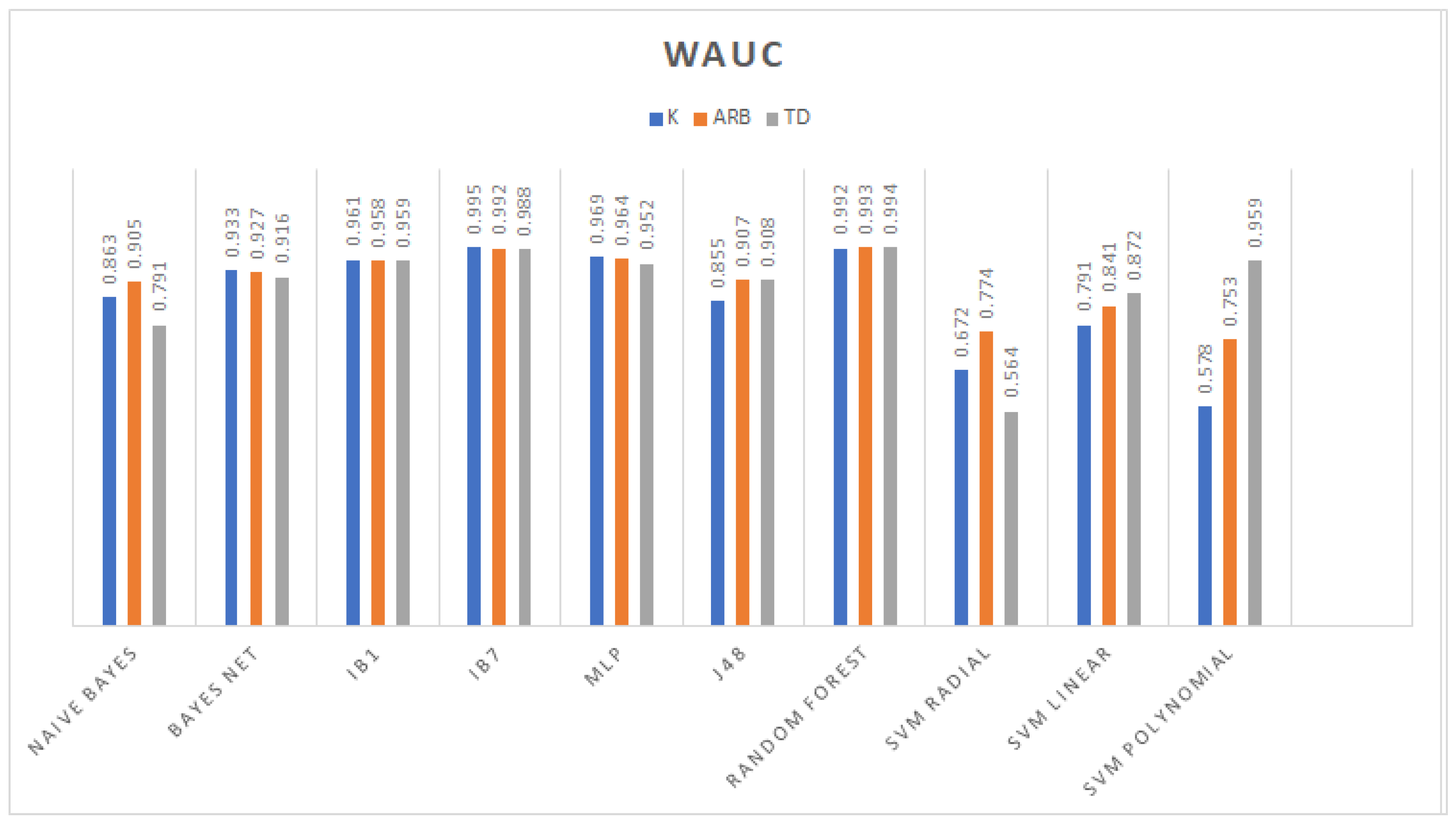
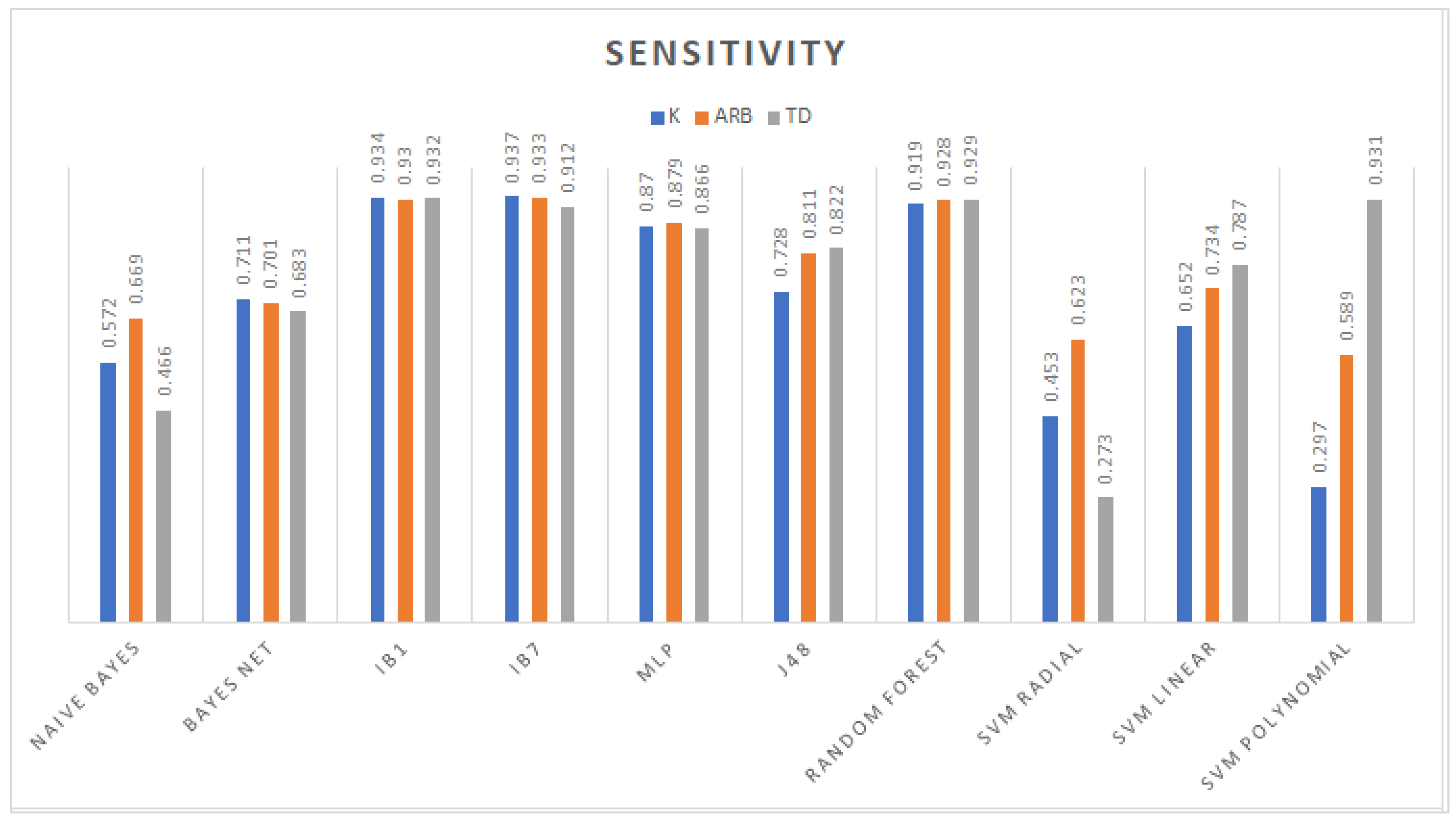
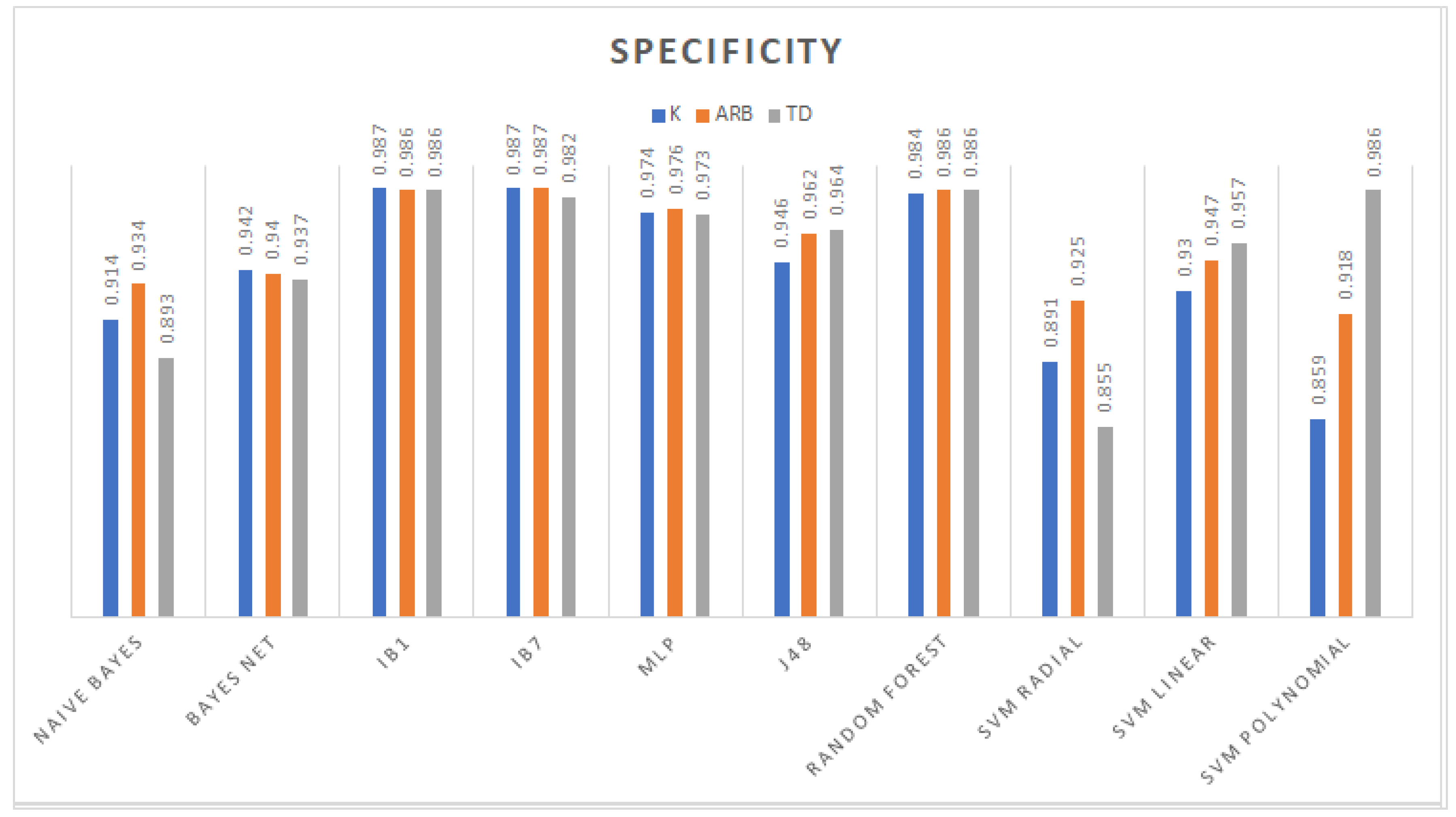
3.1. Classification
3.2. Feature Selection Classification Performance
4. Discussion
5. Conclusions
Author Contributions
Funding
Acknowledgments
Conflicts of Interest
References
- Guo, Y.; Naik, G.R.; Huang, S.; Abraham, A.; Nguyen, H.T. Nonlinear multiscale Maximal Lyapunov Exponent for accurate myoelectric signal classification. Appl. Soft Comput. J. 2015, 36, 633–640. [Google Scholar] [CrossRef]
- De Luca, C.J. Electromyography; John Wiley & Sons, Inc.: Hoboken, NJ, USA, 2006. [Google Scholar] [CrossRef]
- Reaz, M.B.; Hussain, M.S.; Mohd-Yasin, F. Techniques of EMG signal analysis: Detection, processing, classification and applications. Biol. Proced. Online 2006, 8, 11–35. [Google Scholar] [CrossRef]
- Lahmiri, S.; Boukadoum, M. Improved Electromyography Signal Modeling for Myopathy Detection. In Proceedings of the 2018 IEEE International Symposium on Circuits and Systems (ISCAS), Florence, Italy, 27–30 May 2018; pp. 1–4. [Google Scholar] [CrossRef]
- Fuglsang-Frederiksen, A. The role of different EMG methods in evaluating myopathy. Clin. Neurophysiol. 2006, 117, 1173–1189. [Google Scholar] [CrossRef] [PubMed]
- Dostál, O.; Vysata, O.; Pazdera, L.; Procházka, A.; Kopal, J.; Kuchyňka, J.; Vališ, M. Permutation entropy and signal energy increase the accuracy of neuropathic change detection in needle EMG. Comput. Intell. Neurosci. 2018. [Google Scholar] [CrossRef]
- Cler, M.J.; Stepp, C.E. Discrete Versus Continuous Mapping of Facial Electromyography for Human-Machine Interface Control: Performance and Training Effects. IEEE Trans. Neural Syst. Rehabil. Eng. 2015, 23, 572–580. [Google Scholar] [CrossRef]
- Brunelli, D.; Tadesse, A.M.; Vodermayer, B.; Nowak, M.; Castellini, C. Low-cost wearable multichannel surface EMG acquisition for prosthetic hand control. In Proceedings of the 2015 6th International Workshop on Advances in Sensors and Interfaces (IWASI), Gallipoli, Italy, 18–19 June 2015; pp. 94–99. [Google Scholar] [CrossRef]
- Copaci, D.; Serrano, D.; Moreno, L.; Blanco, D.; Copaci, D.; Serrano, D.; Moreno, L.; Blanco, D. A High-Level Control Algorithm Based on sEMG Signalling for an Elbow Joint SMA Exoskeleton. Sensors 2018, 18, 2522. [Google Scholar] [CrossRef] [PubMed]
- Repnik, E.; Puh, U.; Goljar, N.; Munih, M.; Mihelj, M.; Repnik, E.; Puh, U.; Goljar, N.; Munih, M.; Mihelj, M. Using Inertial Measurement Units and Electromyography to Quantify Movement during Action Research Arm Test Execution. Sensors 2018, 18, 2767. [Google Scholar] [CrossRef]
- Merletti, R.; Farina, D. Surface Electromyography: Physiology, Engineering and Applications; John Wiley & Sons, Inc.: Hoboken, NJ, USA, 2016. [Google Scholar] [CrossRef]
- Hsueh, Y.H.; Yin, C.; Chen, Y.H. Hardware System for Real-Time EMG Signal Acquisition and Separation Processing during Electrical Stimulation. J. Med. Syst. 2015, 39, 88. [Google Scholar] [CrossRef]
- Naik, G.R.; Al-Timemy, A.H.; Nguyen, H.T. Transradial Amputee Gesture Classification Using an Optimal Number of sEMG Sensors: An Approach Using ICA Clustering. IEEE Trans. Neural Syst. Rehabil. Eng. 2016, 24, 837–846. [Google Scholar] [CrossRef]
- Resnik, L.; Huang, H.; Winslow, A.; Crouch, D.L.; Zhang, F.; Wolk, N. Evaluation of EMG pattern recognition for upper limb prosthesis control: A case study in comparison with direct myoelectric control. J. Neuroeng. Rehabil. 2018, 15, 23. [Google Scholar] [CrossRef]
- Gu, Y.; Yang, D.; Huang, Q.; Yang, W.; Liu, H. Robust EMG pattern recognition in the presence of confounding factors: Features, classifiers and adaptive learning. Expert Syst. Appl. 2018, 96, 208–217. [Google Scholar] [CrossRef]
- Venugopal, G.; Navaneethakrishna, M.; Ramakrishnan, S. Extraction and analysis of multiple time window features associated with muscle fatigue conditions using sEMG signals. Expert Syst. Appl. 2014, 41, 2652–2659. [Google Scholar] [CrossRef]
- Menon, R.; Di Caterina, G.; Lakany, H.; Petropoulakis, L.; Conway, B.A.; Soraghan, J.J. Study on Interaction between Temporal and Spatial Information in Classification of EMG Signals for Myoelectric Prostheses. IEEE Trans. Neural Syst. Rehabil. Eng. 2017, 25, 1832–1842. [Google Scholar] [CrossRef]
- Nazmi, N.; Abdul Rahman, M.; Yamamoto, S.I.; Ahmad, S.; Zamzuri, H.; Mazlan, S. A Review of Classification Techniques of EMG Signals during Isotonic and Isometric Contractions. Sensors 2016, 16, 1304. [Google Scholar] [CrossRef] [PubMed]
- Chowdhury, R.H.; Reaz, M.B.; Bin Mohd Ali, M.A.; Bakar, A.A.; Chellappan, K.; Chang, T.G. Surface electromyography signal processing and classification techniques. Sensors 2013, 13, 12431–12466. [Google Scholar] [CrossRef] [PubMed]
- Naik, G.R.; Nguyen, H.T. Nonnegative matrix factorization for the identification of EMG finger movements: Evaluation using matrix analysis. IEEE J. Biomed. Health Inform. 2015, 19, 478–485. [Google Scholar] [CrossRef] [PubMed]
- He, J.; Zhang, D.; Jiang, N.; Sheng, X.; Farina, D.; Zhu, X. User adaptation in long-term, open-loop myoelectric training: Implications for EMG pattern recognition in prosthesis control. J. Neural Eng. 2015, 12, 046005. [Google Scholar] [CrossRef]
- Bozkurt, M.R.; Subaşi, A.; Köklükaya, E.; Yilmaz, M. Comparison of AR parametric methods with subspace-based methods for EMG signal classification using stand-alone and merged neural network models. Turk. J. Electr. Eng. Comput. Sci. 2016, 24, 1547–1559. [Google Scholar] [CrossRef]
- Phinyomark, A.; Limsakul, C.; Phukpattaranont, P. Application of wavelet analysis in EMG feature extraction for pattern classification. Meas. Sci. Rev. 2011, 11, 45–52. [Google Scholar] [CrossRef]
- Veer, K.; Sharma, T. A novel feature extraction for robust EMG pattern recognition. J. Med. Eng. Technol. 2016, 40, 149–154. [Google Scholar] [CrossRef]
- Liu, Y.H.; Huang, H.P.; Weng, C.H. Recognition of Electromyographic Signals Using Cascaded Kernel Learning Machine. IEEE/ASME Trans. Mechatron. 2007, 12, 253–264. [Google Scholar] [CrossRef]
- Naik, G.R.; Kumar, D.K.; Jayadeva. Twin SVM for gesture classification using the surface electromyogram. IEEE Trans. Inf. Technol. Biomed. 2010, 14, 301–308. [Google Scholar] [CrossRef] [PubMed]
- Al-Angari, H.M.; Kanitz, G.; Tarantino, S.; Cipriani, C. Distance and mutual information methods for EMG feature and channel subset selection for classification of hand movements. Biomed. Signal Process. Control 2016, 27, 24–31. [Google Scholar] [CrossRef]
- Khezri, M.; Jahed, M. A Neuro–Fuzzy Inference System for sEMG-Based Identification of Hand Motion Commands. IEEE Trans. Ind. Electron. 2011, 58, 1952–1960. [Google Scholar] [CrossRef]
- Ruangpaisarn, Y.; Jaiyen, S. SEMG signal classification using SMO algorithm and singular value decomposition. In Proceedings of the 2015 7th International Conference on Information Technology and Electrical Engineering: Envisioning the Trend of Computer, Information and Engineering, Chiang Mai, Thailand, 29–30 October 2015. [Google Scholar]
- Sapsanis, C.; Georgoulas, G.; Tzes, A.; Lymberopoulos, D. Improving EMG based classification of basic hand movements using EMD. In Proceedings of the Annual International Conference of the IEEE Engineering in Medicine and Biology Society, Osaka, Japan, 3–7 July 2013; pp. 5754–5757. [Google Scholar] [CrossRef]
- Zhai, X.; Jelfs, B.; Chan, R.H.; Tin, C. Self-recalibrating surface EMG pattern recognition for neuroprosthesis control based on convolutional neural network. Front. Neurosci. 2017, 11, 379. [Google Scholar] [CrossRef] [PubMed]
- Gu, Z.; Zhang, K.; Zhao, W.; Luo, Y. Multi-Class Classification for Basic Hand Movements; Technical Report; University of California San Diego: La Jolla, CA, USA, 2017. [Google Scholar]
- Delsys. Bagnoli TM 2-Channel Handheld EMG System User’s Guide; Technical Report; Delsys Incorporated: Natick, MA, USA, 2018. [Google Scholar]
- De Luca, C.J.; Kuznetsov, M.; Gilmore, L.D.; Roy, S.H. Inter-electrode spacing of surface EMG sensors: Reduction of crosstalk contamination during voluntary contractions. J. Biomech. 2012, 45, 555–561. [Google Scholar] [CrossRef]
- Perotto, A.; Delagi, E.F. Anatomical Guide for the Electromyographer: The Limbs and Trunk; Charles C. Thomas: Springfield, IL, USA, 2011; p. 377. [Google Scholar]
- Hermens, H.J.; Freriks, B.; Disselhorst-Klug, C.; Rau, G. Development of recommendations for SEMG sensors and sensor placement procedures. J. Electromyogr. Kinesiol. 2000, 10, 361–374. [Google Scholar] [CrossRef]
- Haykin, S.S. Adaptive Filter Theory; Pearson: London, UK, 2014. [Google Scholar]
- Burg, J.P. Maximum entropy spectral analysis. SEP6 1975. [Google Scholar] [CrossRef]
- Witten, I.H.; Frank, E.; Trigg, L.; Hall, M.; Holmes, G.; Cunningham, S.J. Weka: Practical Machine Learning Tools and Techniques with Java Implementations. In Proceedings of the ICONIP/ANZIIS/ANNES’99 Workshop on Emerging Knowledge Engineering and Connectionist-Based Information Systems, University of Otago, Dunedin, New Zealand, 22–23 November 1999; pp. 192–196. [Google Scholar]
- Frank, E.; Hall, M.A.; Witten, I.H. The WEKA Workbench Data Mining: Practical Machine Learning Tools and Techniques; Elsevier: Amsterdam, The Netherlands, 2016. [Google Scholar] [CrossRef]
- Ciaccio, E.J.; Dunn, S.M.; Akay, M. Biosignal Pattern Recognition and Interpretation Systems. IEEE Eng. Med. Biol. Mag. 1994. [Google Scholar] [CrossRef]
- Wolpert, D.H.; Macready, W.G. No free lunch theorems for optimization. IEEE Trans. Evol. Comput. 1997, 1, 67–82. [Google Scholar] [CrossRef]


| Feature | Abbreviation | |
|---|---|---|
| 1 | Root mean squared value | RMS |
| 2 | Mean average value | MAV |
| 3 | Variance | VAR |
| 4 | Willison amplitude | WAMP |
| 5 | Wavelength | WL |
| 6 | Auto-regressive | AR |
| 7 | Difference absolute mean value | DAMV |
| 8 | Difference absolute standard deviation value | DASDV |
| 9 | Difference absolute variance | DVARV |
| 10 | Difference absolute standard deviation | DASDV |
| 11 | Second order moment | M2 |
| 12 | Integrated EMG | IEMG |
| 13 | Simple squared integration | SSI |
| 14 | Myopulse percentage rate | MYOP |
| 15 | Cepstral coefficients | CC |
| 16 | Log detector | LOG |
| 17 | Temporal moment | TK |
| 18 | V order | V |
| 19 | Zero crossings | ZC |
| 20 | Slope sign change | SSC |
| Research Group | Algorithm | Accuracy |
|---|---|---|
| [32] | Neural Network after Empirical Mode Decomposition (EDM) | 85% |
| [32] | Adaptive Boosting after EMD | 55% |
| [32] | Linear Discriminant Analysis after EMD | 65% |
| [32] | Random Forest after EMD | 91% |
| [32] | Random Forest + PCA after EMD | 94% |
| [29] | Singular-Value Decomposition with SVM | 98.22% |
| [29] | k-Nearest Neighbor | 94.77% |
| [29] | Naive Bayes | 91.66% |
| [29] | Radial Basis Function Network | 94% |
| l | r | Remaining Features |
|---|---|---|
| 29 | 1 | [MAV, SSI, VAR, RMS, WL, WAMP, SSC, ZC, MYOP, Arb:Arb, K:K] |
| 28 | 2 | [SSI, VAR, RMS, WL, WAMP, SSC, ZC, MYOP, Arb:Arb, K:K |
| 27 | 3 | [VAR, RMS, WL, WAMP, SSC, ZC, MYOP, Arb:Arb, K:K] |
| ⋮ | ⋮ | ⋮ |
| 10 | 20 | [ZC, MYOP, Arb, Arb, Arb, Arb, Arb, K, K, K] |
| N | Dataset | Bayes | IBk | MLP | Tree | SVM | |||||
|---|---|---|---|---|---|---|---|---|---|---|---|
| − | − | − | |||||||||
| 20 | TD | ||||||||||
| 20 | Arb | ||||||||||
| 20 | k |
| N | Features | Bayes | IBk | MLP | Tree | SVM | |||||
|---|---|---|---|---|---|---|---|---|---|---|---|
| − | − | − | |||||||||
| 40 | |||||||||||
| 40 | |||||||||||
| 60 | X |
| N | Features | Bayes | IBk | MLP | Tree | SVM | |||||
|---|---|---|---|---|---|---|---|---|---|---|---|
| − | − | − | |||||||||
| 26 | |||||||||||
| 26 | |||||||||||
| 20 | |||||||||||
| 8 | |||||||||||
| 8 | |||||||||||
| 8 | |||||||||||
| 8 |
© 2019 by the authors. Licensee MDPI, Basel, Switzerland. This article is an open access article distributed under the terms and conditions of the Creative Commons Attribution (CC BY) license (http://creativecommons.org/licenses/by/4.0/).
Share and Cite
Ramírez-Martínez, D.; Alfaro-Ponce, M.; Pogrebnyak, O.; Aldape-Pérez, M.; Argüelles-Cruz, A.-J. Hand Movement Classification Using Burg Reflection Coefficients. Sensors 2019, 19, 475. https://doi.org/10.3390/s19030475
Ramírez-Martínez D, Alfaro-Ponce M, Pogrebnyak O, Aldape-Pérez M, Argüelles-Cruz A-J. Hand Movement Classification Using Burg Reflection Coefficients. Sensors. 2019; 19(3):475. https://doi.org/10.3390/s19030475
Chicago/Turabian StyleRamírez-Martínez, Daniel, Mariel Alfaro-Ponce, Oleksiy Pogrebnyak, Mario Aldape-Pérez, and Amadeo-José Argüelles-Cruz. 2019. "Hand Movement Classification Using Burg Reflection Coefficients" Sensors 19, no. 3: 475. https://doi.org/10.3390/s19030475
APA StyleRamírez-Martínez, D., Alfaro-Ponce, M., Pogrebnyak, O., Aldape-Pérez, M., & Argüelles-Cruz, A.-J. (2019). Hand Movement Classification Using Burg Reflection Coefficients. Sensors, 19(3), 475. https://doi.org/10.3390/s19030475