Electromagnetic Modeling and Structure Optimization of a Spherical Force Sensing System

1
School of Automation Science and Electrical Engineering, Beihang University, Beijing 100191, China
2
Shenzhen Institute of Beihang, Shenzhen 518057, China
*
Author to whom correspondence should be addressed.
Sensors 2019, 19(3), 552; https://doi.org/10.3390/s19030552
Submission received: 30 November 2018
/
Revised: 20 January 2019
/
Accepted: 22 January 2019
/
Published: 29 January 2019
(This article belongs to the Special Issue Mechatronic Systems for Automatic Vehicles)
Abstract
:Force sensing system (FSS) is widely used to simulate the control force of aircrafts for pilots. Conventional FSS employs multiple single-axis motors and complex transmission mechanisms to achieve multiple degree-of-freedom (DOF) force output of joystick, which may cause mismatched inertia and affect the output performance of FSS significantly. Therefore, one novel FSS with multiple DOF direct-drive spherical actuator is proposed in this paper to reduce the simulator’s extra inertia. To analyze its output performance systematically, a hybrid modeling method is proposed to formulate both Ampere torque and cogging torque mathematically. Equivalent current method along with Ampere force law is used to obtain the Ampere torque due to irregular structure of magnet and coil poles. The cogging torque is then obtained from airgap flux density via Maxwell stress method. From the derived analytical model, an adaptive particle swarm optimization (PSO) algorithm based on expectation (the average value of minimum errors) is proposed for multiple-parameter structure optimization. It can avoid local optimization effectively. The study shows that the optimized value greatly helps to improve the torque generation. Then, one research prototype and one testbed is developed. The comparison between experimental result and analytical model shows that the two sets of data fit with each other well. Therefore, the analytical model could be employed for motion control of the system at the next stage.
1. Introduction
Force sensing system (FFS) is an aircraft utility device to provide pilots with the sense of control force feedback from the rudder load [1,2,3]. It plays an extremely important role in generating the most intuitive information of aircraft status [4,5,6]. In flight simulators, the performance of FSS directly affects the training result of pilots and the performance evaluation of aircrafts. FSS is generally categorized into digital hydraulic and digital electric types [7,8]. Compared with the digital hydraulic system, the digital electric system can effectively reduce energy loss and environmental pollution. It is the major development trend of FSS in the future [9,10,11]. The digital electric FSS designed by Prendergast et al. is composed of a linear motor, digital computer, and position loop force sensor, etc. However, the employment of the linear motor driver increases the system volume and mass [12]. Wang et al. developed an electric FSS in which the motor adjusts the system stiffness according to the force model to control the joystick force sense [13,14]. Due to the complexity of the system, the inertia force is large. However, damping force and inertia force are not studied.
The inertia-redundant force greatly affects the performance of FSS [15,16]. Traditional FSSs require multiple single-axis motors, connecting rods, gears, worms and other components [17,18]. The complex structure yields large inertia-redundant force, and thus compromises the output performance of servo system unavoidably.
Therefore, this paper proposes a novel FSS driven by spherical actuator with two-dimensional (2D) camber Halbach array to reduce the inertia-redundant force [19,20,21]. Spherical actuator is an electric device capable of achieving multiple DOF rotary motions in a single joint [22,23,24]. Compared with conventional FSS, it has compact structure [25,26], lower moment inertia, and fast response [27,28]. A hybrid approach is proposed to formulate the torque output of the spherical actuator analytically. The equivalent current method along with Ampere force law is used to obtain the Ampere torque due to irregular structures of magnet and coil poles. The cogging torque is then obtained from airgap flux density between rotor and stator via Maxwell stress method. Following that, based on the derived analytical model, an adaptive particle swarm optimization (PSO) algorithm [29,30] based on expectation is proposed for multiple-parameter structure optimization. For traditional PSO algorithms, it is difficult to confirm particle number before optimization, which may lead to local optimum value instead of global value [31,32]. The proposed adaptive PSO algorithm can modify particle quantity based on iterating effect, and achieve global optimum value. The simulation results show that it can solve the problem of particle number initialization, and the optimized values can improve the system output performance greatly. Based on the optimum parameter values, one research prototype and one testbed are developed. Experiments are conducted on the torque generation of the FSS. It shows that the analytical model fits with the experimental results well. Therefore, the validated analytical torque solution could be used for future studies on motion-control implementations. The comparison with traditional spherical actuator shows that the novel design with 2D camber Halbach array greatly improves the output torque. It also provides torque ripple that allows pilots to perceive the variation of rudder load. The comparison further verifies that the novel FSS can reduce the inertia-redundant force effectively.
The rest of this paper is organized as follows. Section 2 presents the design concept and operating principle of the proposed spherical actuator. Section 3 formulates the output torque of 2D longitudinal camber Halbach array analytically. Section 4 optimize the electromagnetic structure parameters based on the adaptive PSO algorithm. Section 5 evaluates torque increase and inertia decrease of the FSS. Section 6 presents the development of research prototype and testbed, and then experimental studies are carried out to validate the analytical solution. Section 7 concludes the research work.
2. Schematic Structure and Operating Principle
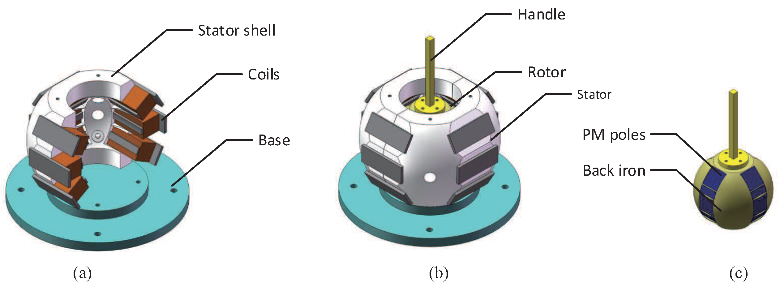
As shown in Figure 1, the schematic structure of the spherical actuator with 2D camber Halbach array and iron stator for FSS of flight simulators is presented. It is mainly composed of one spherical shell-like stator and one rotor housed inside. Four sets of permanent magnet (PM) poles are mounted and evenly distributed along the circumferential direction of the rotor. Each set includes five poles magnetized in radial and tangential directions constituting 2D camber Halbach array on a spherical surface. Similarly, four sets of coils are mounted on the stator along the circumference of the stator, each consisting of three coils in the longitudinal direction.
As shown in Figure 2, the operating principle of the proposed spherical actuator is illustrated. The interaction between magnetic field of rotor poles and current input of stator coils generates attraction or repulsion forces, and thus produces inclination torque on the rotor. Ferromagnetic material is employed for the stator and rotor design to reduce the magnetic energy loss and thus improve the output performance. It is especially useful for the implementation of joysticks in aircrafts.
3. Torque Modeling of Force Sensing System
3.1. Magnetic Field Model with Full Sets of Magnets
As shown in Figure 3, to define a spherical coordinate system [22], we choose two orthogonal directions, the zenith and an origin point at the rotor center. This choice determines a reference plane that contains the origin and is perpendicular to the zenith. The spherical coordinates of a point A are then defined as follows: the radial distance r is the distance from the origin O to A; the inclination (or polar angle) is the angle between the z axis and the line segment ; the azimuth (or azimuthal angle) is the signed angle measured from the x axis to the orthogonal projection of the line segment on the reference plane.
As shown in Figure 2 and Figure 3, to formulate the magnetic field distribution, the actuator space under study is divided into four regions: (1) outer air layer; (2) radial PM poles; (3) back iron of rotor; (4) tangential PM poles. The full sets of magnets are considered simultaneously to formulate the magnetic field distribution around the rotor surface.
We assume that the ferromagnetic material works in the linear portion without hysteresis, and the permeability of ferromagnetic material is much greater than that of air gap [33]. Considering the boundary condition between radial and tangential poles, spherical harmonics function can represent the magnetic flux density of magnetic poles. Therefore, the three components of the magnetic flux density can be obtained as
where , , are three components of magnetic flux density produced by the PM pole; and are residual magnetization of radial and tangential PMs; is permeability of free space; is angle between radial and tangential PM, , , , , and are coefficients obtained based on the spherical harmonic equation and boundary conditions.
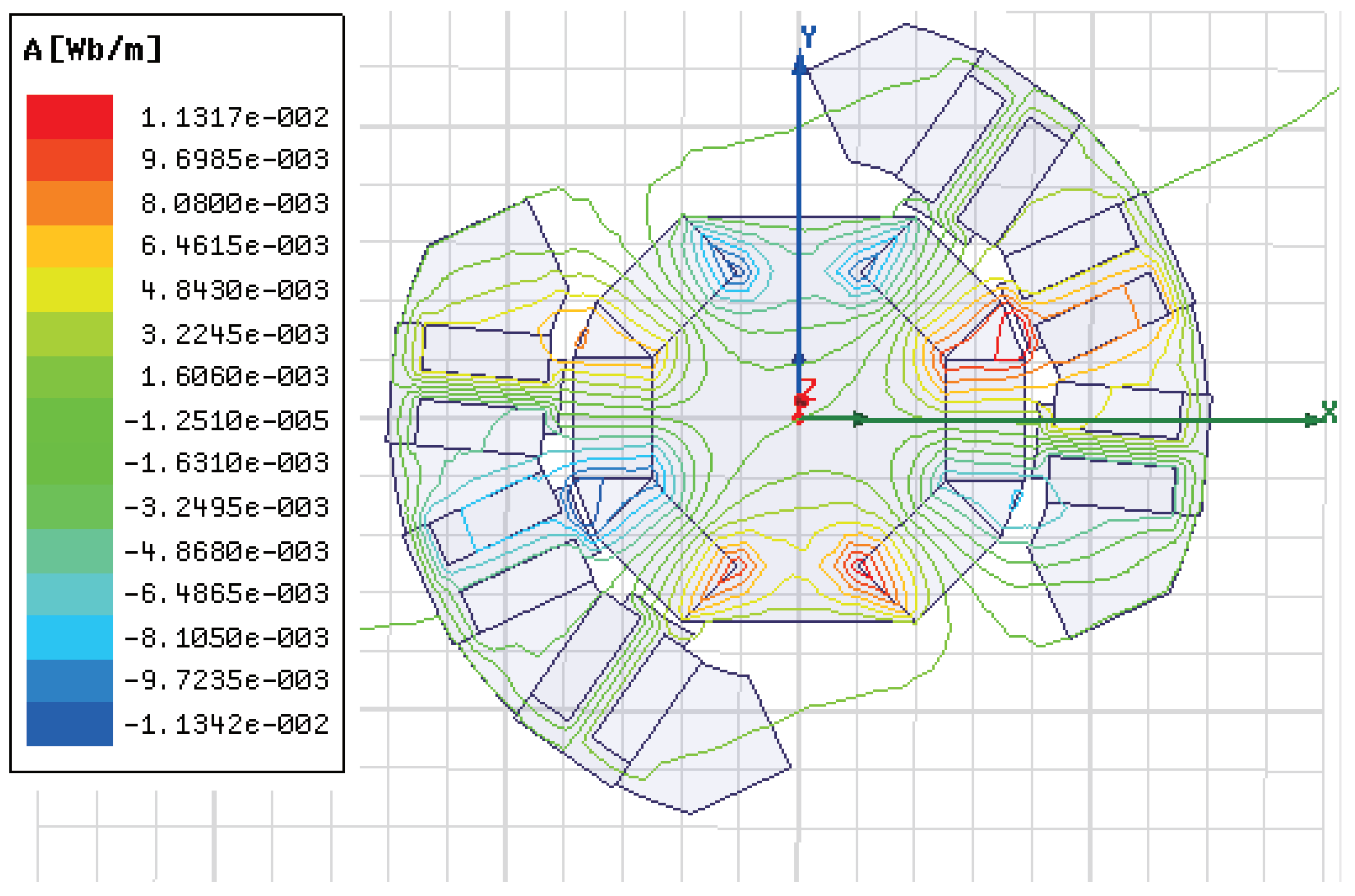
The cross-sectional drawing of the magnetic circuit is shown in Figure 4. It can be found that the magnetic flux generated by PMs forms a close loop through the magnets, the air gap, the coils, the stator shell, and the rotor core. Only small amount of magnetic leakage is not connected by back iron. The magnetic flux energized by coils follows similar distribution between the rotor and the stator. The employment of the rotor iron core and the stator iron shell helps to reduce magnetic leakage and improve the system output performance.
To obtain the output torque generated by one coil, we assume the coil consists of numerous differential segments. It can be verified that only the radial component can produce magnetic torque. and do not produce magnetic torque on the rotor, because the Ampere force generated by them passes through the rotor center. The total torque by one coil can be obtained by integrating the differential torque in the coil volume. The similar approach is employed by other researchers [34] In addition, based on the principle of Maxwell stress equation, cogging torque is generated by and . Therefore, the subsequent torque study will focus on and .
3.2. Torque Generated by Single Coil
To facilitate the calculation of Ampere force, the stator windings are equivalent to magnets and PMs are equivalent to coils. The coil assumes a conical-shaped object embedded in the stator shell to facilitate the formulation of the actuator torque [35]. The magnetic flux density generated by the stator winding is
where , and are respectively the magnetic flux area of the iron core, coil and winging, and are respectively the permeability of iron core and coil, and are respectively the length of iron core and coil, and N is the number of winding turns. is the coil current shown as follows:
where i is magnitude of current input, is angular displacement of actuator. In PM pole,
where is equivalent surface current density of PM pole, and is flux density of PM pole. Let , , thus,
where is differential equivalent surface current of PM pole, and is differential area of PM pole. Hence, we have
where is Ampere force of i-th PM pole in angular displacement, is equivalent cross-sectional area in angular displacement, is equivalent segment of PM pole [36,37]. Thus, the torque generated by a single coil can be obtained as
where and are components of torque, is equivalent cross-sectional area in angular displacement, and R is rotor radius. Since the radial force does not produce torque, we have where torque component
Thus, the total electromagnetic torque by a single coil is
3.3. Cogging Torque of Single Coil
According to Maxwell’s stress equation, we can obtain two formulas of magnetic force between magnets as
where and are respectively the normal and tangential components of the magnetic field force, is differential area of coil cross section and and are respectively the normal and tangential components of the magnetic flux density. In this study, the magnetic field between the iron core and the PM generates the magnetic cogging force. Since the radial magnetic field force does not produce torque, we only consider the tangential force. We can simplify the Maxwell stress formulation as follows:
where is the magnetic flux density of PM pole, is the angle between the PM pole and z-axis. Thus,
where is magnetic cogging force of i-th iron core, and are respectively the normal and tangential components of the magnetic flux density of i-th iron core, and is the magnetic flux area of winging. Thus, the torque generated by a single winding can be obtained as
where and are components of cogging torque, , and are three components of PM magnetic flux density, and R is rotor radius. Since the radial magnetic field force does not produce torque, we obtain radial torque as
Thus, the total cogging torque by a single coil is
3.4. Torque Generated by Full Set of Coils
By summing whole coils’ torque based on the Ampere formula, we obtain the torque in direction is
where , and are equivalent cross-sectional area of i-th PM. Thus, the x-axis component of the electromagnetic torque of the entire actuator is
where
Therefore, the output torque of the actuator is
where is the x-axis component of total cogging torque, , , and are components of PM magnetic flux density in r direction, and , and are components of PM magnetic flux density in direction. Equation (22) represents the torque component in single direction. The overall electromagnetic torque is
Considering the cogging torque of the actuator, the actual output torque of the 2-DOF actuator is
4. Structure Optimization Based on Adaptive PSO Algorithm
4.1. Adaptive PSO Algorithm with Expectation and Deviation
4.1.1. Traditional PSO Algorithm
Traditional PSO can be expressed as follows: assume a particle swarm composed of m particles in a dimensional search space; the position of particle i is defined as , where D is dimension; the individual optimal position is , its fitness is , and its speed is . The global optimal position is . In this paper, optimization parameters are defined as and . Then, the speed and position of the i-th particle in generation can be calculated iteratively according to the following equations:
where w is inertial weight, , are acceleration coefficients that usually have the same value, and are two random values in the range of [0, 1]. In the optimization, the speed of the particle is usually limited to a range with as its critical value, and the position of the particle is also limited within a certain range. In addition, during the iteration, and are constantly updated so that the optimal solution of can be obtained.
4.1.2. Adaptive PSO Algorithm with Anti-Local Optimization
In traditional PSO algorithm, the particle quantity is difficult to be determined. The calculation result may not meet the accuracy requirement due to improper selection of particle quantity. Therefore, a novel adaptive PSO algorithm with anti-local optimization is proposed. An external nested loop algorithm is embedded to increase or decrease particles quantity in PSO iteration. Then, the PSO algorithm conducts iteration in double learning loops, gradually optimizing the number of particles, at the same time modifying the final error to meet the optimization requirement. The structure of the proposed adaptive algorithm is shown in Figure 5.
The modification rule of particle quantity in the adaptive PSO algorithm is as follows. In the first place, the initial particle quantity in the second layer of PSO algorithm is set by considering the actual situation, in this case 5. Then, the PSO algorithm iterates to modify the number of particles (increase or decrease), until it reaches iteration requirement. The PSO algorithm expectation definition is given as
where P is the total number of particles, L is the particle layer of PSO algorithm, is the generation number of PSO algorithm, Y is the actual output. The expectation is average value of minimum errors and is used to evaluate whether the PSO algorithm achieves the optimization goal. When the PSO iteration number meets the requirement, the attenuation rate D is defined as
In this study, the cost function is
where is minimum distance, is initial constant. The constraint of PSO is
where is error threshold. Define , as the declining rates before and after T-th iteration, , as the predetermined attenuation rates, and , . There are several addition and deletion rules:
- Initialize the parameters of PSO algorithm randomly. When the number of iterations reaches T, calculate ;
- If , i.e., PSO algorithm is convergence, delete 10 particles;
- If , i.e., PSO algorithm performance is perfect, maintain the PSO structure;
- If , i.e., PSO performance is poor, increase 10 particles;
- If and , increase 10 particles; otherwise, maintain the PSO structure.
4.2. Structural Parameter Optimization
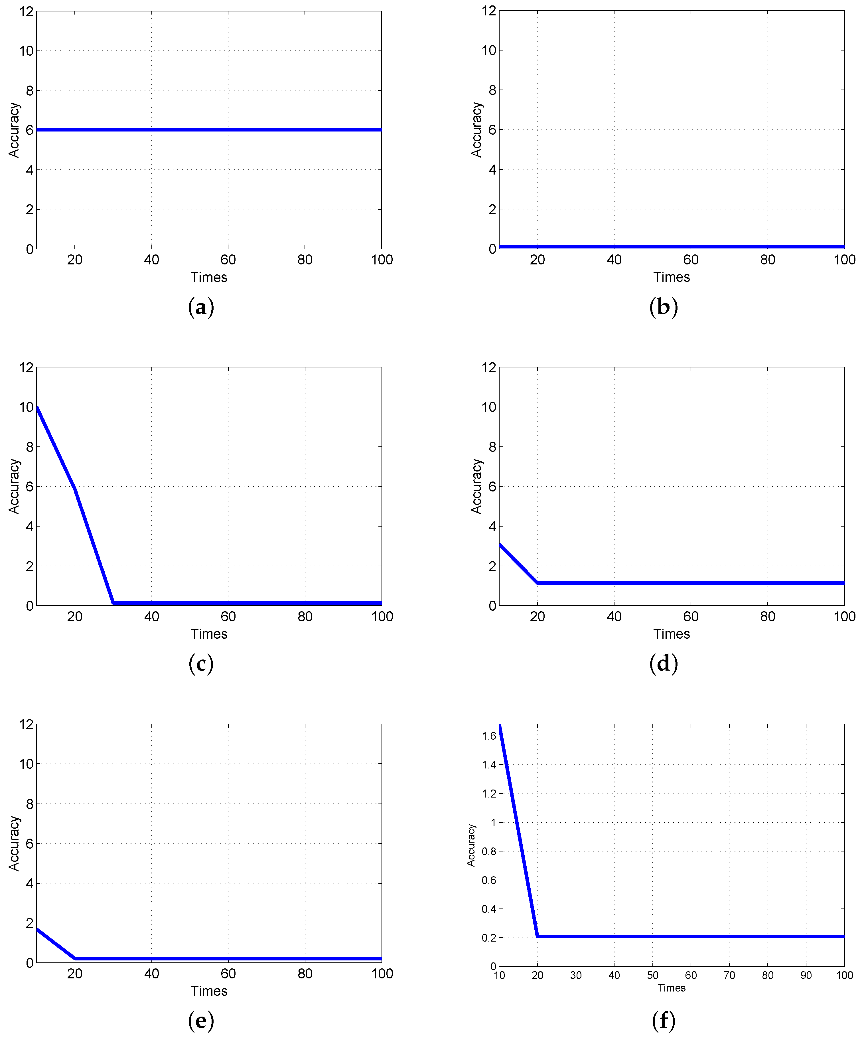
The iteration accuracy curves of PSO from 5 to 35 particles are shown in Figure 6. We find that the accuracy of Figure 6b,c satisfies the requirements, but the algorithm continues to iterate. It indicates that there is a local minimum value. In addition, although PSO particle number of Figure 6c is consistent with that of Figure 6d, parameters in algorithm are not the same. Therefore, the results of two iteration accuracy curve are similar but slightly different. At last, PSO with 35 particles meet the optimization accuracy demand.
The calculation results are shown in Table 1. It includes PSO algorithm expectation , decline rate and . Let the largest decline rate and minimum decline rate be 0.5 and 0.4, respectively. As shown in Table 1, the PSO iteration error rate is less than 0.4. The expectation generated by PSO iteration meets requirements until particles increase from 5 to 35. At the same time, the adaptive PSO stops the iteration. Therefore, the adaptive PSO can determine the particles quantity and avoid local optimization, which deduces the iterations of PSO. The optimization result of major electromagnetic structure parameters is shown in Figure 7.
The electromagnetic parameters of the initial, PSO and Adaptive PSO designs are calculated, and the torque outputs are compared. The comparisons of output torque (positive current), (negative current) and cogging torque are presented in Figure 8. It proves that the electromagnetic torque and cogging torque optimized by Adaptive PSO are better greater than those of initial design. Furthermore, the nonlinearity is found in the torque curve. Because the coil core is made of ferromagnetic material, the torque fluctuation is larger than that of air-core coil. In the case of no current supply, the torque is equal to zero at because the Ampere torque is zero and the direction of the cogging torque is opposite at two sides of rotor equator. When the coils are supplied with power, the superposition of Ampere torque and cogging torque at two sides of rotor equator is no longer equal. Therefore, the resulting torque is not symmetrical around the zero position.
5. Performance Evaluation of the Proposed Design
5.1. Comparison of Torque Output between 2D Longitudinal Camber Halbach Array and Traditional PM Array
The torque output of 2D longitudinal camber Halbach PM array with ferromagnetic structure is compared with that of traditional alternative radial magnetization PM array with air-core coil. The major numerical model parameters is shown in Table 2. The comparison results of (positive current), (negative current) and cogging torque with respect to the longitudinal angle at are presented in Figure 9. It is found that the torque output of the proposed design is much larger than that of traditional design. In the torque comparison, we adopt the same current, magnetic pole volume, rotor volume, and airgap size. Because the novel spherical actuator’s coil core is made of ferromagnetic materials, and the PM array adopts 2D camber Halbach array, the torque output is greatly increased.
Generally, nonlinearity is not preferred for the design of electric actuators. However, the spherical actuator proposed in this paper is applied to the FSS of the flight simulator. The variation of torque with respect to the rotor orientation helps the pilot to feel the external loading from rudders. Therefore, the nonlinearity of output torque is necessary.
5.2. Inertia Moment Comparison between New FSS and Traditional FSS
The inertia moment comparison between new FSS and traditional FSS is shown in Figure 10. Figure 10a shows that with the increase of angular acceleration, the inertia moment of the novel FSS is smaller than that of the traditional FSS. Figure 10b shows that the inertia moment of the new FSS is smaller than that of the traditional FSS with the increase of the motion frequency of the joystick. Therefore, the novel FSS with compact structure greatly reduce the inertia-redundant force caused by the complex transmission mechanism of the traditional FSS.
6. Experimental Investigation of Force Sensing System
6.1. Research Prototype and Testbed
One research prototype is developed as shown in Figure 11. The ball-like rotor is mounted with magnet poles on the surface, and the spherical-shell-like stator is mounted with coils. The rotor is housed inside the stator, and the interaction between magnet poles and the current input in the coils generates torque to move the rotor.
The experimental testbed is shown in Figure 12. The handle of the spherical actuator is mounted with force sensor which in turn is fixed on the arc guide. The handle can change its orientation along with the force sensor, and the torque output can be measured accordingly.
6.2. Comparison of Experimental Results and Analytical Model
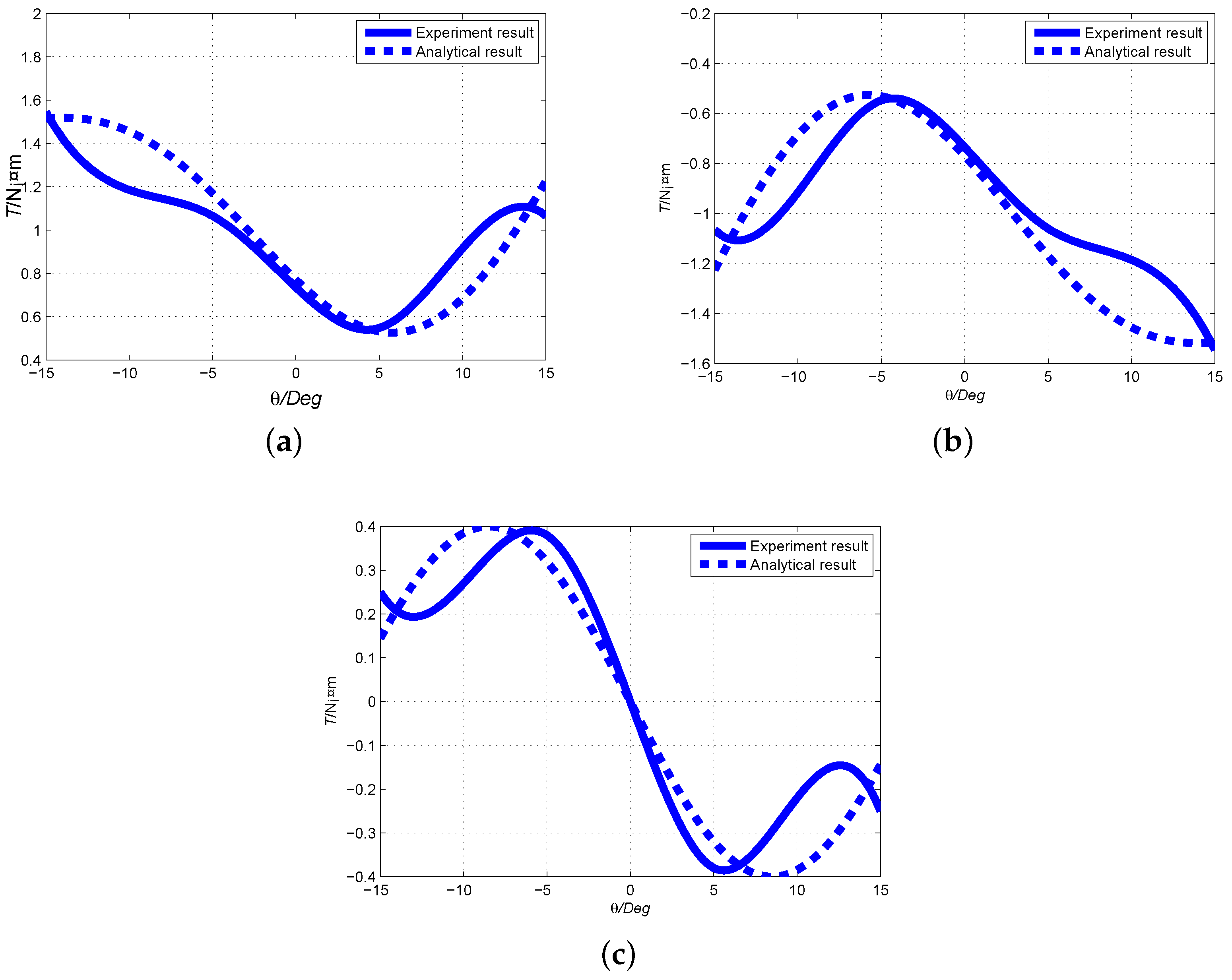
To further observe the variation of torque output and validate the analytical torque model, the experimental results are compared with the analytical model. The same structural parameters are employed for experimental and analytical computations. The comparisons of output torque (positive current), (negative current) and cogging torque are presented in Figure 13.
Figure 13a shows the comparison of analytical model and experimental result of output torque when current direction is positive. In the longitudinal or direction, the variation of output torque creates one peak and one trough values, which is consistent with the magnet arrangement on the rotor surface. The peak values appear at and trough at . It is also found that the analytical model fits with the experimental result of the output torque well. Similarly, Figure 13b presents the variation comparison of analytical model and experimental result of output torque when current is negative. And Figure 13c shows the comparison of analytical model and experimental result of cogging torque . It can be found that the analytical model is also consistent with the experimental result.
Differences of between experimental result and analytical model may be caused by the geometrical approximation of magnet poles, specifically spherical crown entity in analytical model whereas block PM poles for the prototype development due to the convenience of fabrication. The stator shell and coil iron cores are geometrically approximated in analytical model for the convenience of computation.
7. Conclusions
One novel FSS with spherical actuator is proposed in this paper to reduce the simulator’s redundant inertia force. A hybrid approach is employed to formulate the torque output analytically. Specifically, the Ampere torque is modeled from the equivalent current method, and the cogging torque is obtained from Maxwell stress method. Subsequently, an adaptive PSO method with expectation is proposed for design optimization. It can avoid local minimum value, and obtain global optimization conveniently. The simulation result shows that the optimization can improve the torque generation greatly. The torque comparison between the proposed and the traditional designs shows that the former can greatly improve the output torque and provide torque ripple to perceive the variation of rudder load. Compared with the traditional FSS, the proposed one can reduce the inertia-redundant force and improve the torque servo performance. Based on the optimum values, one research prototype as well as one testbed has been developed. Experiments are conducted on the output torque of the research prototype. The experimental result is compared with the analytical model. It shows that the analytical model fits well with the experimental result. Therefore, the validated analytical torque solution could be used for future studies on motion-control implementations.
Author Contributions
Y.L. and L.Y. did major contribution to this paper; they proposed the general framework for the design and analysis of spherical force sensing system; Z.J. gave important suggestion on mathematical modeling.
Funding
This work was supported by the National Key R&D Program of China under grant 2017YFB1300404, the National Natural Science Foundation of China (NSFC) under grant 51575026 and 51875013, the Fundamental Research Funds for the Central Universities, and Science and Technology on Aircraft Control Laboratory.
Conflicts of Interest
The authors declare no conflict of interest.
References
- Coiro, D.; Marco, A.D.; Nicolosi, F. A 6DOF Flight Simulation Environment for General Aviation Aircraft with Control Loading Reproduction. In Proceedings of the AIAA Modeling and Simulation Technologies Conference and Exhibit, Boston, MA, USA, 19–22 August 2013. [Google Scholar]
- Shutao, Z.; Qitao, H.; Dacheng, C.; Junwei, H. Experiment and Study of Control Loading System in a Flight Simulator Based on RCP. In Proceedings of the 2007 IEEE International Conference on Integration Technology, Shenzhen, China, 20–24 March 2007; pp. 208–212. [Google Scholar]
- Zhao, J.; Shen, G.; Yang, C.; Liu, G.; Yin, L.; Han, J. Feel force control incorporating velocity feedforward and inverse model observer for control loading system of flight simulator. Proc. Inst. Mech. Eng. Part I J. Syst. Control Eng. 2013, 227, 161–175. [Google Scholar] [CrossRef]
- Nam, Y.; Hong, S.K. Force Control System Design for Aerodynamic Load Simulator. Control Eng. Pract. 2002, 10, 549–558. [Google Scholar] [CrossRef]
- Kim, J.W.; Xuan, D.J.; Kim, Y.B. Design of a Forced Control Dystem for a Dynamic Road Simulator Using QFT. Int. J. Automot. Technol. 2008, 9, 37–43. [Google Scholar] [CrossRef]
- Lai, L.J.; Gu, G.Y.; Zhu, L.M. Design and Control of a Decoupled Two Degree of Freedom Translational Parallel Micro-positioning Stage. Rev. Sci. Instrum. 2012, 83, 045105. [Google Scholar] [CrossRef] [PubMed]
- Niksefat, N.; Sepehri, N. Design and Experimental Evaluation of a Robust Force Controller for an Electro-hydraulic Actuator via Quantitative Feedback Theory. Control Eng. Pract. 2000, 8, 1335–1345. [Google Scholar] [CrossRef]
- Ying, L.U.; Wang, Y.L.; Wang, Z.L.; Liang, J.M. Force-Feeling Simulation System of Longitudinal Control Based on the Electro-Motive Force Servo. Acta Simulata Syst. Sin. 2003, 83. [Google Scholar] [CrossRef]
- Fu, J.C.; Liu, X.H.; Ma, T.C. Experiment and Study of Electric Control Loading System. Adv. Mater. Res. 2012, 462, 720–726. [Google Scholar] [CrossRef]
- Gerretsen, A.; Mulder, M. Comparison of Position-loop Velocity-loop and Force-loop Based Control Loading Architectures. In Proceedings of the AIAA Modeling and Simulation Technologies Conference, San Francisco, CA, USA, 15–18 August 2005; pp. 813–827. [Google Scholar]
- John, P. Realistic feel in Flight Simulators is Based on Precise Control Loading. Aircr. Eng. 1983, 55, 10–12. [Google Scholar]
- Prendergast, W.K. Apparatus and Method for Primary Control Loading for Vehicle Simulation. U.S. Patent 5370535, 6 December 1994. [Google Scholar]
- Lu, Y.; Wang, Y.; Sun, F. The Construction and Validation Studies on Principle Prototype of Electric Force-feeling Simulation System. In Proceedings of the International Conference on Computational and Information Sciences, Shiyang, China, 21–23 June 2013; pp. 1048–1051. [Google Scholar]
- Wang, Y.; Lu, Y. Design of Control Load System of Flight Simulator Based on Matlab. Microcomput. Inf. 2006, 22, 56–58. [Google Scholar]
- Hess, R.A. Analyzing Manipulator and Feel System Effects in Aircraft Flight Control. IEEE Trans. Syst. Man Cybern. 1990, 20, 923–931. [Google Scholar] [CrossRef]
- Qi, P.; Wang, H.; Han, J. Stability of Position-loop Based Hydraulic Control Loading System. In Proceedings of the International Conference on Mechanic Automation and Control Engineering, Wuhan, China, 26–28 June 2010; pp. 3363–3366. [Google Scholar]
- Qi, P. Hydraulic Control Loading System Based on Position Control. J. Jilin Univ. 2008, 34, 558–563. [Google Scholar]
- JianYong, Y.; Zongxia, J.; Yaoxing, S.; Cheng, H. Adaptive Nonlinear Optimal Compensation Control for Electro-hydraulic Load Simulator. Chin. J. Aeronaut. 2010, 23, 720–733. [Google Scholar] [CrossRef] [Green Version]
- Sakaidani, Y.; Hirata, K.; Niguchi, N.; Maeda, S. Experimental Verification of Feed-back Control of A 2-DOF Spherical Actuator. IEEE Trans. Magn. 2014, 50, 1–4. [Google Scholar] [CrossRef]
- Lee, K.M.; Son, H. Distributed Multipole Model for Design of Permanent-magnet-based Actuators. IEEE Trans. Magn. 2007, 43, 3904–3913. [Google Scholar] [CrossRef]
- Son, H.; Lee, K.M. Distributed Multipole Models for Design and Control of PM Actuators and Sensors. IEEE/ASME Trans. Mechatron. 2008, 13, 228–238. [Google Scholar] [CrossRef]
- Son, H.; Lee, K.M. Open-loop controller Design and Dynamic Characteristics of A Spherical Wheel motor. IEEE Trans. Ind. Electron. 2010, 57, 3475–3482. [Google Scholar] [CrossRef]
- Wang, J.; Jewell, G.W.; Howe, D. A Novel Spherical Actuator: Design and Control. IEEE Trans. Magn. 1997, 33, 4209–4211. [Google Scholar] [CrossRef]
- Wang, J.; Jewell, G.W.; Howe, D. Analysis, Design and Control of A Novel Spherical Permanent-magnet Actuator. IEEE Proc. Electr. Power Appl. 1998, 145, 61–71. [Google Scholar] [CrossRef]
- Yan, L.; Chen, I.; Yang, G.; Lee, K.M. Analytical and Experimental Investigation on the Magnetic Field and Torque of A Permanent Magnet Spherical Actuator. IEEE/ASME Trans. Mechatron. 2006, 11, 409–419. [Google Scholar]
- Yan, L.; Chen, I.M.; Lim, C.K.; Yang, G.; Lin, W.; Lee, K.M. Hybrid Torque Modeling of Spherical Actuators with Cylindrical-shaped Magnet Poles. Mechatron. (Elsevier J.) 2011, 21, 85–91. [Google Scholar] [CrossRef]
- Rossini, L.; Onillon, E.; Chtelat, O.; Perriard, Y. Hybrid Fem-analytical Force and Torque Models of A Reaction Sphere Actuator. In Proceedings of the 2013 IEEE International Electric Machines and Drives Conference (IEMDC), Chicago, IL, USA, 12–15 May 2013; pp. 694–700. [Google Scholar]
- Yan, L.; Chen, I.M.; Lim, C.K.; Yang, G.; Lin, W.; Lee, K.M. Design and Analysis of A Permanent Magnet Spherical Actuator. IEEE/ASME Trans. Mechatron. 2008, 13, 239–248. [Google Scholar] [CrossRef]
- Liu, B.; Wang, L.; Jin, Y. An Effective PSO-Based Memetic Algorithm for Flow Shop Scheduling. IEEE Trans. Syst. Man Cybern. Part B Cybern. A Publ. IEEE Syst. Man Cybern. Soc. 2007, 37, 18–27. [Google Scholar] [CrossRef]
- Ishaque, K.; Salam, Z.; Amjad, M. An Improved Particle Swarm Optimization (PSO)-Based MPPT for PV With Reduced Steady-State Oscillation. IEEE Trans. Power Electron. 2012, 27, 3627–3638. [Google Scholar] [CrossRef]
- Das, S.; Chaudhuri, S. A Comprehensive Survey on Functional Link Neural Networks and An Adaptive PSO-BP Learning for CFLNN. Neural Comput. Appl. 2010, 19, 187–205. [Google Scholar]
- Wang, Y.; Zhou, J.; Zhou, C. An Improved Self-adaptive PSO Technique for Short-term Hydrothermal Scheduling. Expert Syst. Appl. 2012, 39, 2288–2295. [Google Scholar] [CrossRef]
- Yan, L.; Liu, Y.; Zhang, L.; Zongxia, J.; Gerada, C. Magnetic Field Modeling and Analysis of Spherical Actuator with Two-dimensional Longitudinal Camber Halbach Array. IEEE Trans. Ind. Electron. 2018, 1. [Google Scholar] [CrossRef]
- Reutzsch, B.; Schinkoethe, W. Magnetic Levitation System for Linear Direct Drives based on Lorentz Forces. In Proceedings of the Innovative Small Drives and Micro-motor Systems, 9 Gmm/etg Symposium, Nuremberg, Germany, 19–20 September 2013. [Google Scholar]
- Tsai, M.C.; Yang, C.H. A Flux-Density-Based Electromagnetic Servo System for Real-Time Magnetic Servoing/Tracking. IEEE/ASME Trans. Mechatron. 2008, 13, 249–256. [Google Scholar] [CrossRef]
- Liu, Y.P. On the Relations between Ampere Force and Lorentz Force. Adv. Mater. Res. 2011, 403, 1326–1331. [Google Scholar] [CrossRef]
- Valente, J.; Ou, J.-Y.; Plum, E.; Zheludev, N.I. Reconfigurable metamaterials controlled by Lorentz, ampere and coulomb forces: Towards GHz bandwidth. In Proceedings of the European Conference on Lasers and Electro-Optics, Munich, Germany, 12–16 May 2013. [Google Scholar]
Figure 1.
Structure of FSS with spherical actuator. (a) stator; (b) overview construction; (c) rotor.
Figure 1.
Structure of FSS with spherical actuator. (a) stator; (b) overview construction; (c) rotor.

Figure 2.
Operating principle of spherical actuator.
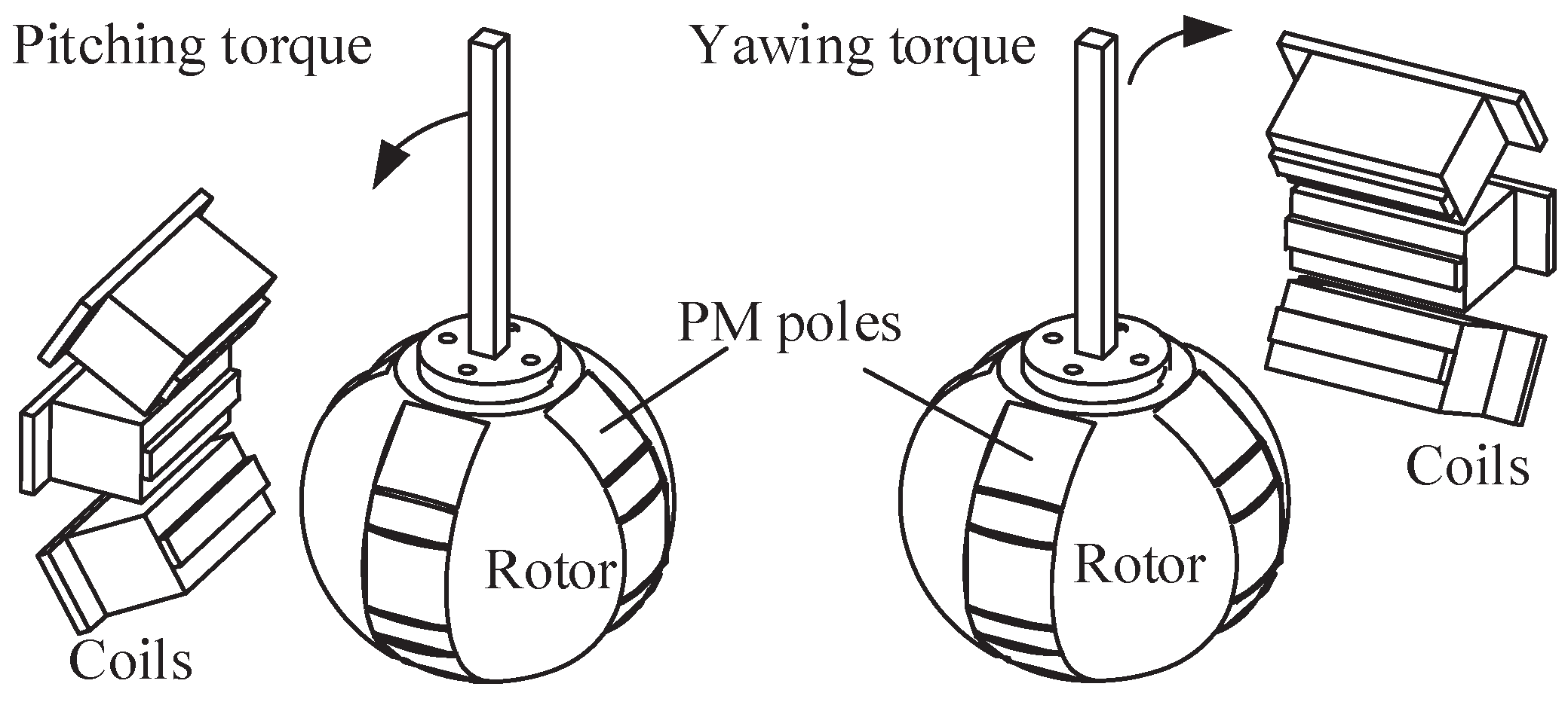
Figure 3.
Distribution of PM poles array.
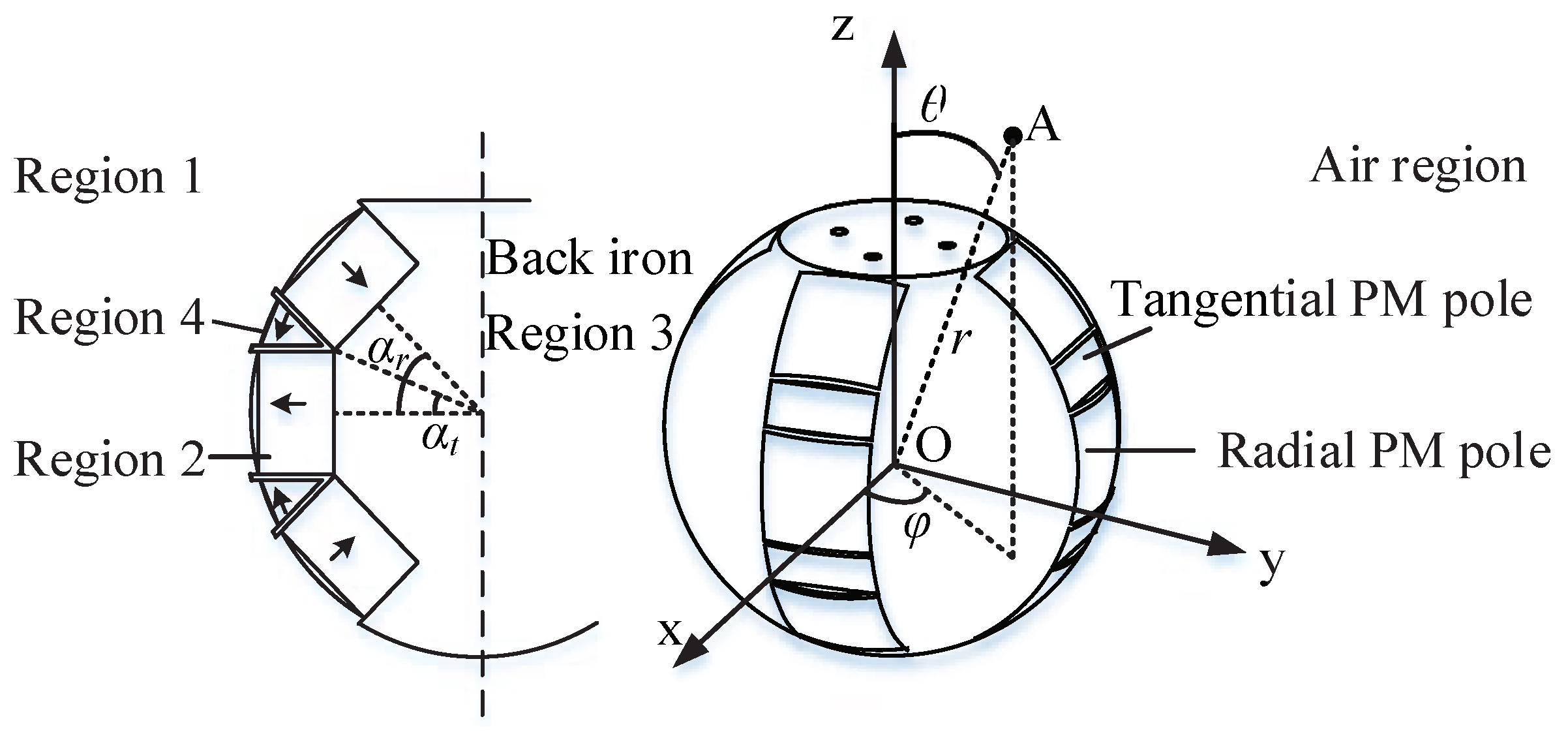
Figure 4.
The cross-sectional drawing of the magnetic circuit.

Figure 5.
Adaptive PSO algorithm structure.
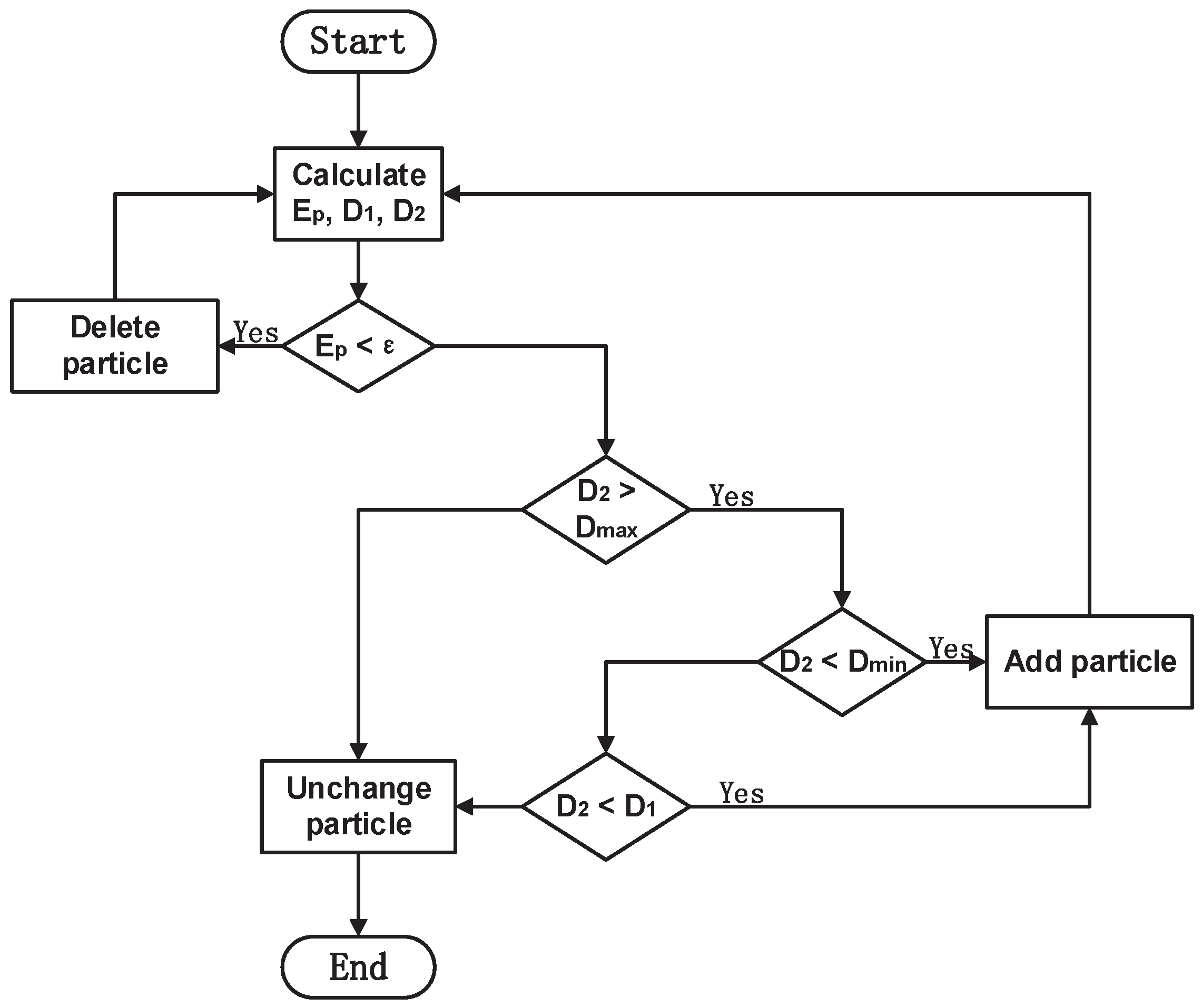
Figure 6.
Optimization accuracy curve based on adaptive PSO algorithm. (a) Optimization accuracy with 5 particles; (b) Optimization accuracy with 15 particles; (c) Optimization accuracy with 25 particles; (d) Optimization accuracy with 25 particles; (e) Optimization accuracy with 35 particles; (f) Optimization accuracy with 35 particles.

Figure 7.
Optimization of electromagnetic structure parameters. (a) Optimization of iron core area; (b) Optimization of coil area; (c) Optimization of electromagnet area.
Figure 7.
Optimization of electromagnetic structure parameters. (a) Optimization of iron core area; (b) Optimization of coil area; (c) Optimization of electromagnet area.

Figure 8.
Optimization comparison of output torque. (a) Optimization comparison of output torque when current direction is positive; (b) Optimization comparison of output torque when current direction is negative; (c) Optimization comparison of output torque .
Figure 8.
Optimization comparison of output torque. (a) Optimization comparison of output torque when current direction is positive; (b) Optimization comparison of output torque when current direction is negative; (c) Optimization comparison of output torque .
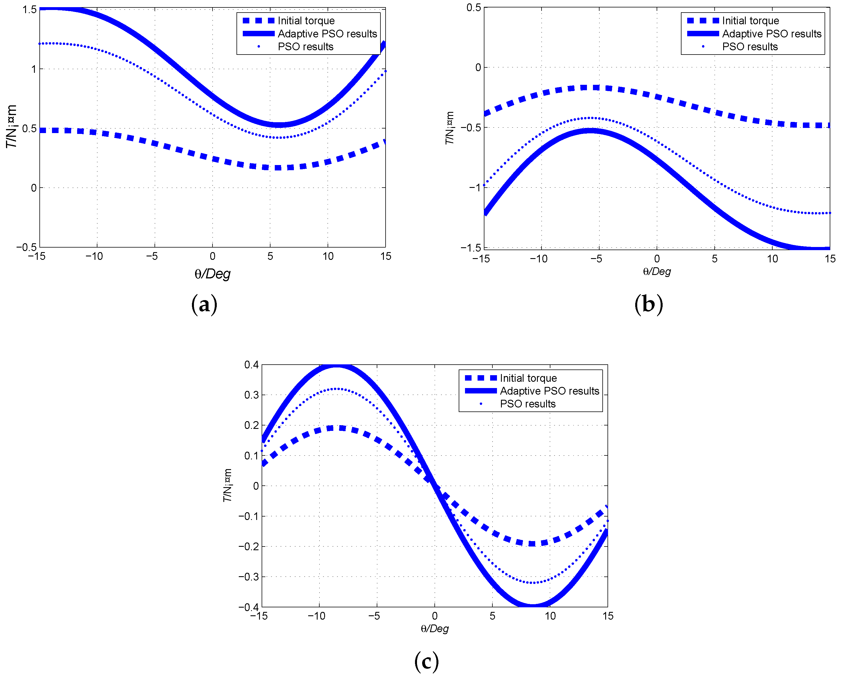
Figure 9.
Comparison of output torque between 2D camber Halbach array and traditional PM array. (a) Output torque when current direction is positive; (b) Output torque when current direction is negative; (c) Output cogging torque .
Figure 9.
Comparison of output torque between 2D camber Halbach array and traditional PM array. (a) Output torque when current direction is positive; (b) Output torque when current direction is negative; (c) Output cogging torque .

Figure 10.
Inertia moment comparison of novel and traditional FSS. (a) Inertia moment under different angular acceleration; (b) Inertia moment changed with motion.
Figure 10.
Inertia moment comparison of novel and traditional FSS. (a) Inertia moment under different angular acceleration; (b) Inertia moment changed with motion.
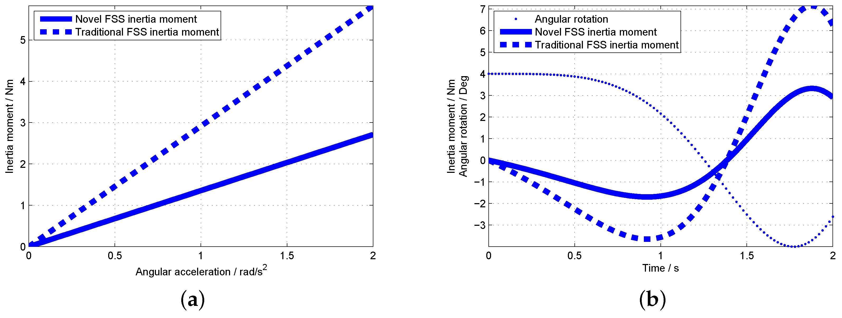
Figure 11.
Overview of the developed research prototype.

Figure 12.
Experimental testbed for the measurement of output torque.
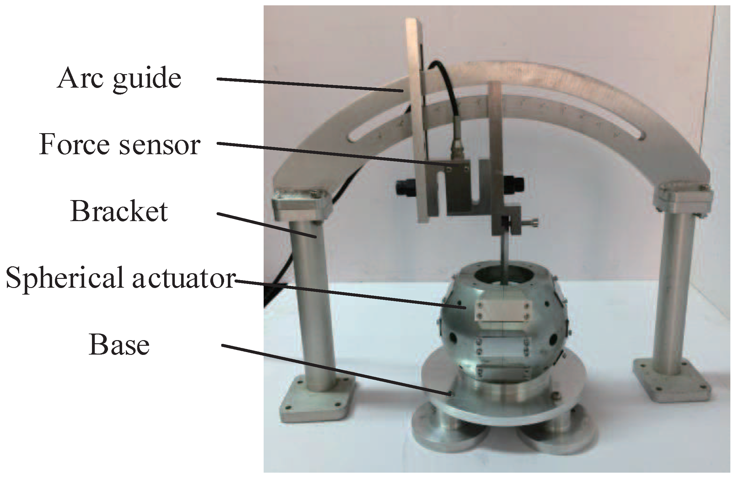
Figure 13.
Comparison of output torque between experiment result and analytical result. (a) Output torque when current direction is positive; (b) Output torque when current direction is negative; (c) Output cogging torque .
Figure 13.
Comparison of output torque between experiment result and analytical result. (a) Output torque when current direction is positive; (b) Output torque when current direction is negative; (c) Output cogging torque .

Table 1.
Comparison between different particle nodes number of adaptive PSO algorithm.
| No. | Particles Number | Expectation | Decline Rate | Decline Rate |
|---|---|---|---|---|
| 1 | 5 | 6.0071 | 0 | 0 |
| 2 | 15 | 0.1053 | 0 | 0.9825 |
| 3 | 25 | 0.1385 | 0.9825 | −0.3152 |
| 4 | 25 | 1.1356 | −0.3152 | −7.1996 |
| 5 | 35 | 0.2068 | −7.1996 | 0.8179 |
Table 2.
Key parameters of the prototype.
| Stator | Stator radius/(mm) | 70 |
| Number of stator coils poles | 12 | |
| Iron core area/(mm) | 425 | |
| Coil area/(mm) | 1000 | |
| Electromagnet area/(mm) | 2050 | |
| Electromagnet angle/() | 30 | |
| Coil turn number | 200 | |
| Coil width/(mm) | 20 | |
| Rotor | Rotor radius /(mm) | 40 |
| PM pole parameters /() | 45 | |
| PM pole parameters /() | 22.5 | |
| Number of rotor PM poles | 20 | |
| PM pole thickness/(mm) | 15 | |
| PM pole width/(mm) | 10 |
© 2019 by the authors. Licensee MDPI, Basel, Switzerland. This article is an open access article distributed under the terms and conditions of the Creative Commons Attribution (CC BY) license (http://creativecommons.org/licenses/by/4.0/).
Share and Cite
MDPI and ACS Style
Yan, L.; Liu, Y.; Jiao, Z. Electromagnetic Modeling and Structure Optimization of a Spherical Force Sensing System. Sensors 2019, 19, 552. https://doi.org/10.3390/s19030552
AMA Style
Yan L, Liu Y, Jiao Z. Electromagnetic Modeling and Structure Optimization of a Spherical Force Sensing System. Sensors. 2019; 19(3):552. https://doi.org/10.3390/s19030552
Chicago/Turabian StyleYan, Liang, Yinghuang Liu, and Zongxia Jiao. 2019. "Electromagnetic Modeling and Structure Optimization of a Spherical Force Sensing System" Sensors 19, no. 3: 552. https://doi.org/10.3390/s19030552
Note that from the first issue of 2016, this journal uses article numbers instead of page numbers. See further details here.