Abstract
This paper addresses the challenge of enhancing range precision in radar sensors through supervised learning. However, when the range precision surpasses the range resolution, it leads to a rapid increase in the number of labels, resulting in elevated learning costs. The removal of background noise in indoor environments is also crucial. In response, this study proposes a methodology aiming to increase range precision while mitigating the issue of a growing number of labels in supervised learning. Neural networks learned for a specific section are reused to minimize learning costs and maximize computational efficiency. Formulas and experiments confirmed that identical fractional multiple patterns in the frequency domain can be applied to analyze patterns in other FFT bin positions (representing different target positions). In conclusion, the results suggest that neural networks trained with the same data can be repurposed, enabling efficient hardware implementation.
1. Introduction
Radar is a sensor that uses reflected waves from objects to determine the target range. Radar sensors are widely used to obtain various information such as the distance, position, speed, and material type of objects. As the application fields of radar sensors become more diverse, there is a noticeable trend of demanding high performance even in inexpensive radar sensors. Among the performance requirements for low-cost radar sensors, distance accuracy is the most crucial, and various research efforts are needed to enhance this capability. The more accurate the range precision, the higher the possible performance in cars, drones, security facilities, IoT equipment, etc. The accuracy of a target range with FMCW radar is determined by the range resolution, which in turn depends on the bandwidth of the radar waveform. A wider bandwidth leads to higher range resolution, and bandwidth depends on the waveform generated by the oscillator. However, an oscillator with a wide bandwidth incurs high costs. Signal processing algorithms enable the enhancement of radar range resolution while maintaining cost efficiency. In this paper, the terms range resolution and range precision are used as follows: range resolution refers to the minimum unit that can distinguish between multiple targets, indicating different objects. Range precision is used as the unit that accurately represents the position of a single target. The most commonly used algorithm is zero padding [1]. Alternative algorithms include the use of n-point mirrors or phase padding on time-domain (TD) samples [2]. Padding can improve the range accuracy of the Fourier transform (FT) by taking more samples within the coherence processing interval (CPI).
Within indoor environments, the noise floor must be considered. This term refers to reflected waves, multipath interference, and signals from objects such as indoor walls and pillars, which can mask the desired signal [3,4,5]. Discontinuities in the time-domain signal lead to phase errors, resulting in clutter noise in the frequency domain and a reduction in the range precision [3,6]. In [7], index-based distance estimation (IBDE) trains the beat frequency pattern associated with each label, effectively reducing range precision errors. It ensures the prevention of discontinuities, even in the absence of background interference. Additionally, there is no need to increase the FFT points since the number of samples does not increase. The IBDE method employs supervised learning which necessitates acquiring and organizing a sufficient amount of data for each label. Consequently, the issue of labeling has been raised, particularly regarding cost, leading to the investigation of various methods [8,9,10]. FMCW radar also encounters limitations owing to the labeling issue. This is because the supervised learning model requires labeling for each beat frequency index. This paper introduces a method to address the labeling concern while efficiently reusing neural networks to enhance range precision in FMCW radar.
2. Fundamental FMCW Radar Waveform
FMCW radar uses signals that increase in frequency over time. Figure 1 shows the FMCW sawtooth signal. Tx refers to the transmitted signal and Rx refers to the received signal. refers to the round-trip delay time of the target. is the beat frequency, is sampling period, and N is the number of FFT points. Additionally, is the beat frequency, is the chirp period, is the sampling period, and N represents the number of FFT points.
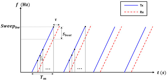
Figure 1.
FMCW radar waveform.
Figure 2 delineates the signal processing procedure employed to derive the target distance from the radar. The voltage-controlled oscillator (VCO) generates a FMCW waveform, which is subsequently transmitted by Tx after passing through a low noise amplifier (LNA). The signal received by Rx is then mixed with the VCO-generated signal and amplified. Subsequently, the beat frequency is extracted by eliminating the carrier component through a low-pass filter (LPF). The amplitude of the received signal in the frequency domain determines the target range. Equation (1) represents the beat signal post LPF processing, as depicted in Figure 2.
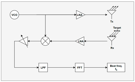
Figure 2.
Signal processing flow in FMCW radar.
In the radar signal processing, represents the beat frequency formed by mixing the transmitted and received signals [11]. is the Fourier transform of . A is the amplitude of the transmitted signal, and σ means the amplitude attenuation attributed to radar cross-section and path loss. The variable R denotes the target range.
Equation (3) represents the beat frequency as the fast Fourier transform (FFT) of a discrete frequency signal. Here, Fs is defined as 1/Ts, where denotes the FFT bin number. In Equation (4), the parameter signifies the argument at which the magnitude of is maximal.
3. Proposed Algorithm
In radar signal processing, when the target’s range R is an integer multiple of the range resolution, it can be expressed using Equation (5). Applying Equation (5) from Equation (2) results in the expression given by Equation (7). In this paper, we consider the target range by separating it into integer multiples and fractional multiples of the range resolution. The target range () can be expressed by Equation (6), where n is the integer multiple range, consistent with the n used in Equation (5), and γ represents the radar’s range resolution. The parameter p defines the fractional multiple range. Substituting this into Equation (2) results in the simplified form presented as Equation (8). It signifies the sinc shift by K. When p equals zero, Sf(n) exhibits zero-crossing sidelobes. Otherwise, for non-zero values of p, Sf(n) follows a sinc shape, where the sidelobes are dependent on the term K. Hence, the sidelobes of Sf(n) shifted by p are dependent on the term K. That is, the sinc pattern of Sf(n) is determined by the term K and is independent of n.
N in Equation (6) is the number of FFT points. Figure 3 shows the results of a simulation when p is fixed while n varies. The experiment environment has a range resolution of = 0.3 m, p = 0.2 m, and n = 11, 15, and 21 in an ideal environment. The most significant ratios between the two peaks were about 82%, 83%, and 85%, respectively, and the ratio of the increase and decrease patterns were revealed through a simple experiment.
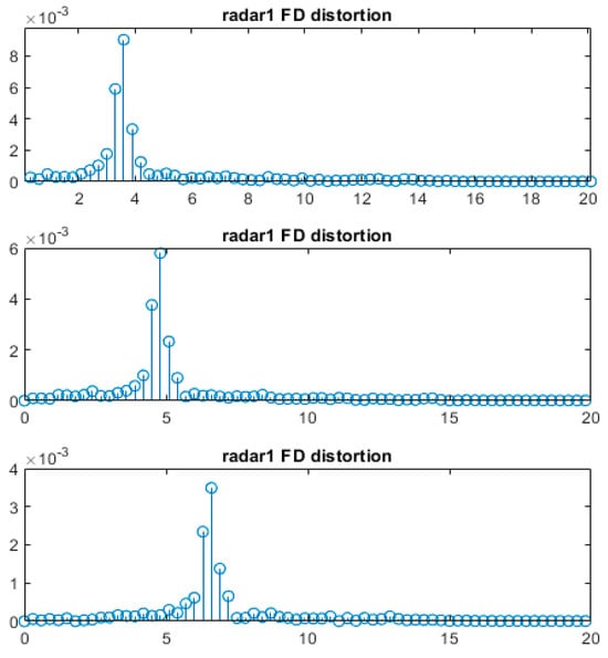
Figure 3.
Spectrum for ranges of 3.5 m, 4.7 m, and 6.5 m with a 0.3 m of radar range resolution in a MATLAB simulation. Each axis represents bin numbers and frequency magnitude.
3.1. Frequency Shift
Equation (8) demonstrates the independence of the target’s fractional multiple range from n. Therefore, the proposed approach focuses solely on learning for the fractional multiple range (). The term of can be frequency-shifted for an arbitrary integer (). It serves as the reference value for a frequency shift. Equations (9)–(11) show frequency shift calculation. is the peak index or CFAR detected index. is the difference between and . is the frequency difference multiplied by the bin step , and N denotes the number of FFT points. Figure 4 illustrates the frequency shift using a diagram. The diagram indicates that it is composed of the number of m labels, in which each label represents the distance index with the distance resolution of the bin interval () divided by m. When the beat frequency signal is moved by the frequency shift, all instances of n become .
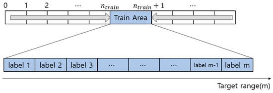
Figure 4.
Training area and labels.
3.2. Power Normalization and Noise Floor Cancellation
Power normalization is performed to cover the path loss according to the frequency shift. Path loss compensation should be achieved through max peak normalization, avoiding the use of a relational expression. Training data are obtained by measuring within the training region shown in Figure 5. The frequency-shifted signal differs in magnitude from the training data, primarily due to path loss. Power normalization involves dividing the signal by its maximum magnitude. The inference data perform power normalization to mitigate the impact of path loss. This normalization process is applied to the training data to match the main lobe’s magnitude between the two signals. Peak normalization allows the pattern to focus on the sidelobes, which imply a fractional times p in Equation (6). In addition, noise floor cancellation reduces the impact of the environment by removing background noise from the target’s spectrum [3]. In the training and inference phase of the neural network model, Gaussian filters of range resolution size were used to mitigate the effects of integer multiples [12].
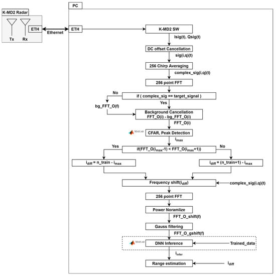
Figure 5.
Proposed algorithm flow.
3.3. Deep Learning Architecture
3.3.1. Architecture
In this paper, the neural network of the FMCW radar is based on a convolutional neural network (CNN). Figure 6 illustrates the proposed CNN architecture designed for inferring radar labels. The input layer utilizes a power-normalized 256-point spectrum. The convolutional layer incorporates 8, 16, and 32 1 × 1 mask filters for each respective layer [13,14,15,16,17,18]. Batch normalization is performed after each convolutional layer, followed by the rectified linear unit activation function [19,20]. The pooling layer has a 1 × 1 pool size and a stride of 2 [21]. Subsequently, the data are fully connected to the m neurons [22,23]. Each neuron calculates the probability for each label via SoftMax, and the reference label is output through the classification layer.
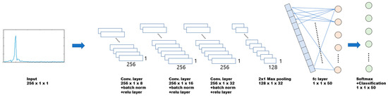
Figure 6.
Proposed CNN algorithm.
3.3.2. Data Augmentation
Training data were created using MATLAB simulations. The range resolution was 0.3 m, was 20, m was 50, and was 0.006 m. The position and label of the target had a 1:1 correspondence. The training data added a random range corresponding to 10% of the label range. A thousand data points were used per label. In assuming an indoor environment, the Rician multipath and additive white Gaussian noise were added. Phase error was introduced to the simulation to emulate real-world conditions, with an offset of approximately ±20 ppm from the carrier frequency [2]. Training was conducted using MATLAB, resulting in a training accuracy of 60% and a loss of 1. The accuracy of the label, however, does not show the distance error, and the mean average error was obtained through experiments. Figure 7 and Figure 8 show how to gather the training dataset and the training results, respectively.
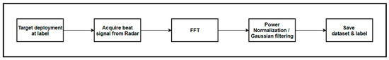
Figure 7.
Flow to make a training dataset.
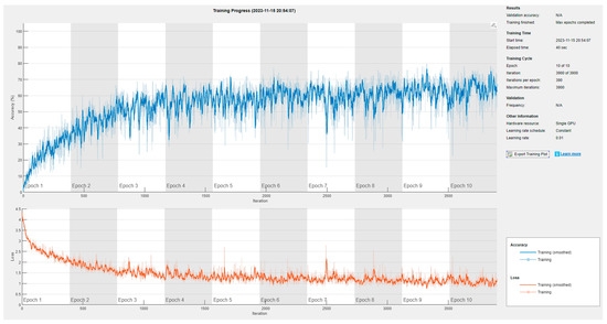
Figure 8.
CNN training result.
3.3.3. Inference and Restore Integer Range
The label output from CNN is converted to distance through Equation (12). is the range that has been improved by the proposed algorithm.
4. Experiments
4.1. Environment
Measurements were conducted in a hallway at Sejong University to validate the proposed algorithm in a real-world setting. The employed radar was an RF-beam K-MD2 FMCW radar, starting at a frequency of 24 GHz with a swept bandwidth of 500 MHz and a range resolution of 0.3 m given in Table 1 [24]. The Gaussian filter used had a 3 dB bandwidth in the impulse response of 1.48 MHz, with an impulse length of 8 samples per symbol and 17 sample points [25,26]. A total of 50,000 training datasets were employed, with each dataset comprising 1000 data points for each label. Figure 9 illustrates the experimental environment. The experiment was conducted by varying the target position within the range of 3 m to 16 m.

Table 1.
Experiment parameters.
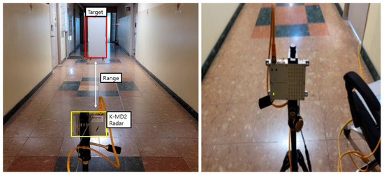
Figure 9.
Test environment.
4.2. Experiment Result
Figure 10 depicts the outcomes obtained by applying the proposed algorithm to the experimental data utilizing real radar measurements. The x-axis represents the distance between the target and the radar, while the y-axis illustrates the disparity between the measured and actual values. The ground truth was acquired through a laser measuring instrument with a precision of ±2 mm. The mean average error (MAE) given in Equation (13) was determined to be 0.07 m.
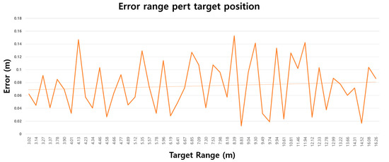
Figure 10.
Range estimation results on real targets experiments. (the dotted line = average).
E denotes the range errors between the ground truth and the proposed algorithm’s range, while S represents the number of tests conducted. Table 2 displays the performance comparison with IBDE. The range precision achieved by the proposed method was 0.06 m, calculated as 0.3 m divided by 50. CMAE is calculated by multiplying MAE with CR (compensate rate). CR is an index designed to compensate for range resolution, as per Equation (14), where represents the bandwidth of the reference radar, and is the bandwidth of the target radar [27,28]. The CMAE serves as an index that adjusts for the MAE based on the radar’s range resolution, facilitating a comparison of the algorithm’s improvement rate. The proposed algorithm has advantages in label spacing compared to related works [7,13,29]. The experimental results demonstrate the effectiveness of the proposed algorithm within the 3–16 m range. The experiments were conducted at intervals of approximately 10 cm, offering more refined measurements compared to earlier studies [7,13,29]. Equation (14) was formulated for analyzing the performance and experimental results.
Table 2.
Comparison of experimental results for algorithms.
FFT bin spacing refers to the distance between the bins of a signal obtained by performing an n-point FFT on a beat frequency. The bin represents the target location more accurately than the label. If the mean absolute error (MAE) is less than the bin spacing, the bin can be considered to be precisely pointing to the target. Conversely, if the MAE is greater than the bin spacing, the bin is not correctly pointing to the target. Range precision must be determined by taking the MAE into account. In CASE2, the position of the target is accurately expressed rather than the label spacing. Similarly, if the MAE is smaller than the label spacing, the label accurately indicates the target, and in the opposite case, the range precision should be determined by considering the MAE. According to Equation (15), the range precision of the algorithm was 0.07 m.
In Equation (15), range precision(m) can be simplified depending on the relations between FFT bin spacing(m) and label spacing(m) as the following:
5. Conclusions
This paper addressed the challenge posed by the increasing number of labels resulting from the expansion of the operating range by employing a frequency shift. It introduced a methodology that achieves a broad operating range and high range precision relative to the number of labels. Additionally, the algorithm mitigated clutter by eliminating the noise floor in the frequency domain. The algorithm also reused the training complexity of convolutional neural networks (CNNs) specifically for constant sections. Experimental validation of the algorithm was conducted using FMCW radar measurements. Testing utilized a radar with a range resolution of 0.3 m demonstrated a range precision approximately 4.3 times superior to that of a related work [7]. Through a combination of formulas and experiments, this study demonstrated that identical fractional multiple patterns could be applied to different bin positions using just one fractional pattern. This suggested that neural networks trained on the same data could be efficiently reused for diverse target positions, enabling cost-effective hardware implementation. The experimental results underscored the efficiency and utility of the proposed algorithm for commercial radar sensors, where enhancing performance with minimal hardware costs is a critical concern. However, the limitation of this paper lies in conducting verification solely to discover if the proposed methodology is effective in an actual radar environment. Additional research is needed to optimize such various variables as neural architecture, learning data, number of labels, and power normalization depending on the range resolution.
Author Contributions
Conceptualization, S.L.; Formal analysis, H.C.; Investigation, H.C. and S.L.; Methodology, S.L. and Y.J.; Project administration, S.L.; Software, H.C.; Supervision, S.L.; Writing—original draft, H.C.; Writing—review and editing, Y.J. and S.L. All authors have read and agreed to the published version of the manuscript.
Funding
This research was supported by Institute of Information and Communications Technology Planning and Evaluation (IITP) under the metaverse support program to nurture the best talents (No. IITP-2023-RS-2023-00254529) grant funded in part by the Korea government (MSIT), in part by the Basic Science Research Program through the National Research Foundation of Korea (NRF) funded by the Ministry of Education (No. 2020R1A6A1A03038540), and in part by an NRF grant funded by the Korea government (MSIT) (No. 2023R1A2C1006340); the EDA tools were supported by the IC Design Education Center (IDEC), Korea.
Institutional Review Board Statement
Not applicable.
Informed Consent Statement
Not applicable.
Data Availability Statement
Data are contained within the article.
Conflicts of Interest
The authors declare no conflict of interest.
References
- Qi, G. High accuracy range estimation of FMCW level radar based on the phase of the zero-padded FFT. In Proceedings of the 7th International Conference on Signal Processing, 2004. Proceedings. ICSP '04. 2004, Beijing, China, 31 August–4 September 2004; Volume 3, pp. 2078–2081. [Google Scholar] [CrossRef]
- Baek, S.; Jung, Y.; Lee, S. Signal Expansion Method in Indoor FMCW Radar Systems for Improving Range Resolution. Sensors 2021, 21, 4226. [Google Scholar] [CrossRef]
- Yang, S.; Kim, Y. Single 24-GHz FMCW Radar-Based Indoor Device-Free Human Localization and Posture Sensing with CNN. IEEE Sens. J. 2023, 23, 3059–3068. [Google Scholar] [CrossRef]
- Li, W.; Li, Y.; Zhang, J.; Lu, J.; Dong, S.; Gu, C.; Mao, J. A Feature-based Filtering Algorithm with 60GHz MIMO FMCW Radar for Indoor Detection and Trajectory Tracking. In Proceedings of the 2023 IEEE/MTT-S International Microwave Symposium—IMS 2023, San Diego, CA, USA, 11–16 June 2023; pp. 427–430. [Google Scholar] [CrossRef]
- Sharma, P.; Gaba, S.P.; Singh, D. Study of background subtraction for ground penetrating radar. In Proceedings of the 2015 National Conference on Recent Advances in Electronics & Computer Engineering (RAECE), Roorkee, India, 13–15 February 2015; pp. 101–105. [Google Scholar] [CrossRef]
- Pan, M.; Chen, B.; Yang, M. A General Range-Velocity Processing Scheme for Discontinuous Spectrum FMCW Signal in HFSWR Applications. Int. J. Antennas Propag. 2016, 2016, 2609873. [Google Scholar] [CrossRef]
- Dimitrakakis, C.; Savu-Krohn, C. Cost-Minimising Strategies for Data Labelling: Optimal Stopping and Active Learning. In FoIKS 2008: Foundations of Information and Knowledge Systems; Hartmann, S., Kern-Isberner, G., Eds.; Lecture Notes in Computer Science; Springer: Berlin/Heidelberg, Germany, 2008; Volume 4932. [Google Scholar] [CrossRef]
- Mendez, J.; Schoenfeldt, S.; Tang, X.; Valtl, J.; Cuellar, M.P.; Morales, D.P. Automatic Label Creation Framework for FMCW Radar Images Using Camera Data. IEEE Access 2021, 9, 83329–83339. [Google Scholar] [CrossRef]
- Kim, J.; Ju, J.; Feldt, R.; Yoo, S. Reducing DNN labelling cost using surprise adequacy: An industrial case study for autonomous driving. In Proceedings of the 28th ACM Joint Meeting on European Software Engineering Conference and Symposium on the Foundations of Software Engineering (ESEC/FSE 2020), Online, 8–13 November 2020; Association for Computing Machinery: New York, NY, USA; pp. 1466–1476. [Google Scholar] [CrossRef]
- Liu, J.; Gu, C.; Zhang, Y.; Mao, J.-F. Suppressing Coupling and Stationary Clutters in FMCW Radars with Temporal Filtering. In Proceedings of the 2020 IEEE Asia-Pacific Microwave Conference (APMC), Hong Kong, China, 8–11 December 2020; pp. 348–350. [Google Scholar] [CrossRef]
- Park, K.-E.; Lee, J.-P.; Kim, Y. Deep Learning-Based Indoor Distance Estimation Scheme Using FMCW Radar. Information 2021, 12, 80. [Google Scholar] [CrossRef]
- Knott, E.F.; Schaeffer, J.F.; Tulley, M.T. Radar Cross Section; SciTech Publishing: Raleigh, NC, USA, 2004. [Google Scholar]
- Park, H.; Kim, M.; Jung, Y.; Lee, S. Method for Improving Range Resolution of Indoor FMCW Radar Systems Using DNN. Sensors 2022, 22, 8461. [Google Scholar] [CrossRef] [PubMed]
- Le Cun, Y.; Boser, B.; Denker, J.S.; Henderson, D.; Howard, R.E.; Hubbard, W.; Jackel, L.D. Handwritten Digit Recognition with a Back-Propagation Network. In Advances in Neural Information Processing Systems 2; Touretzky, D., Ed.; Morgan Kaufmann: San Francisco, CA, USA, 1990. [Google Scholar]
- Le Cun, Y.; Bottou, L.; Bengio, Y.; Haffner, P. Gradient-Based Learning Applied to Document Recognition. Proc. IEEE 1998, 86, 2278–2324. [Google Scholar] [CrossRef]
- Murphy, K.P. Machine Learning: A Probabilistic Perspective; MIT Press: Cambridge, MA, USA, 2012. [Google Scholar]
- Glorot, X.; Bengio, Y. Understanding the Difficulty of Training Deep Feedforward Neural Networks. In Proceedings of the Thirteenth International Conference on Artificial Intelligence and Statistics, AISTATS, Sardinia, Italy, 13–15 May 2010; pp. 249–356. [Google Scholar]
- He, K.; Zhang, X.; Ren, S.; Sun, J. Delving Deep into Rectifiers: Surpassing Human-Level Performance on ImageNet Classification. In Proceedings of the 2015 IEEE International Conference on Computer Vision, Cambridge, MA, USA, 7–13 December 2015; IEEE Computer Vision Society: Washington, DC, USA; pp. 1026–1034. [Google Scholar]
- Ioffe, S.; Szegedy, C. Batch Normalization: Accelerating Deep Network Training by Reducing Internal Covariate Shift. arXiv 2015. [Google Scholar] [CrossRef]
- Nair, V.; Hinton, G.E. Rectified linear units improve restricted boltzmann machines. In Proceedings of the 27th International Conference on Machine Learning (ICML-10), Haifa, Israel, 21–24 June 2010; pp. 807–814. [Google Scholar]
- Nagi, J.; Ducatelle, F.; Di Caro, G.A.; Ciresan, D.; Meier, U.; Giusti, A.; Nagi, F.; Schmidhuber, J.; Gambardella, L.M. Max-Pooling Convolutional Neural Networks for Vision-based Hand Gesture Recognition. In Proceedings of the IEEE International Conference on Signal and Image Processing Applications (ICSIPA2011), Kuala Lumpur, Malaysia, 16–18 November 2011. [Google Scholar]
- Saxe, A.M.; McClelland, J.L.; Ganguli, S. Exact solutions to the nonlinear dynamics of learning in deep linear neural networks. arXiv 2013, arXiv:1312.6120. [Google Scholar]
- Bishop, C.M. Pattern Recognition and Machine Learning; Springer: New York, NY, USA, 2006. [Google Scholar]
- RFbeam. K-MD2 Radar Transceiver. 2018. Available online: https://rfbeam.ch/download/k-md2-datasheet/?tmstv=1696875210 (accessed on 10 November 2023).
- Krishnapura, N.; Pavan, S.; Mathiazhagan, C.; Ramamurthi, B. A baseband pulse shaping filter for Gaussian minimum shift keying. In Proceedings of the 1998 IEEE International Symposium on Circuits and Systems (ISCAS), Monterey, CA, USA, 31 May–3 June 1998; Volume 1, pp. 249–252. [Google Scholar]
- Rappaport, T.S. Wireless Communications: Principles and Practice, 2nd ed.; Prentice Hall: Upper Saddle River, NJ, USA, 2002. [Google Scholar]
- Neemat, S.; Uysal, F.; Krasnov, O.; Yarovoy, A. Reconfigurable Range-Doppler Processing and Range Resolution Improvement for FMCW Radar. IEEE Sens. J. 2019, 19, 9294–9303. [Google Scholar] [CrossRef]
- Kim, B.-S.; Lee, J.; Kim, S. SNR and Resolution Improvement Algorithm with the Concatenation of Multiple Chirps for FMCW Radar. IEEE Antennas Wirel. Propag. Lett. (Early Access Article) 2023, 1–5. [Google Scholar] [CrossRef]
- Park, K.; Lee, J.; Kim, Y. Deep Learning-Based Indoor Two-Dimensional Localization Scheme Using a Frequency-Modulated Continuous Wave Radar. Electronics 2021, 10, 2166. [Google Scholar] [CrossRef]
Disclaimer/Publisher’s Note: The statements, opinions and data contained in all publications are solely those of the individual author(s) and contributor(s) and not of MDPI and/or the editor(s). MDPI and/or the editor(s) disclaim responsibility for any injury to people or property resulting from any ideas, methods, instructions or products referred to in the content. |
© 2023 by the authors. Licensee MDPI, Basel, Switzerland. This article is an open access article distributed under the terms and conditions of the Creative Commons Attribution (CC BY) license (https://creativecommons.org/licenses/by/4.0/).