Self-Diagnostic and Self-Compensation Methods for Resistive Displacement Sensors Tailored for In-Field Implementation ^†

Abstract

This paper presents a suitably general model for resistive displacement sensors where the model parameters depend on the current sensor conditions, thereby capturing wearout and failure, and proposes a novel fault detection method that can be seamlessly applied during sensor operation, providing self-diagnostic capabilities. On the basis of the estimation of model parameters, an innovative self-compensation method is derived to increase the accuracy of sensors subject to progressive wearout. The proposed model and methods have been validated by both numerical simulations and experimental tests on two real resistive displacement sensors, placed in undamaged and faulty conditions, respectively. The fault detection method has shown an accuracy of 97.2%. The position estimation error is < ±0.2% of the full-scale span for the undamaged sensor, while the self-compensation method successfully reduces the position estimation error from ±15% to approximately ±2% of the full-scale span for the faulty sensor.

1. Introduction

Displacement sensors are widely used in different applications and fields, such as industrial [1,2], medical [3,4] and automotive [5,6]. Within the industrial field, the role of displacement sensors in control applications is gaining importance since the degree of industrial automation is continuously growing. In this context, there is a constant interest in displacement sensors with increasing intelligence, robust measurement methods, and improved performances [7]. In particular, sensor reliability in producing accurate measurement data is crucial. Augmenting sensor diagnostic capabilities plays an increasingly important role, as undetected failures may negatively affect the industrial process into which the sensor is inserted, resulting in efficiency loss, downtimes or even threatening life safety [8].

Several solutions can be considered to prevent sensor failure and enhance sensor diagnostic coverage. A first approach is the adoption of a Preventive Maintenance (PM) policy, which implies sensor calibration and maintenance activities run on a regular time basis to avoid failures before they occur [9]. Determining in advance when a sensor will enter the wearout phase is challenging, as predictions typically rely on a theoretical failure rate rather than on the current sensor conditions. While PM can reduce unexpected process downtime, it can lead to costly and unnecessary procedures and repairs.

A second possible approach involves employing Fault Detection and Identification (FDI) theory [10,11,12,13]. FDI techniques recognize system faults in process components by monitoring system inputs and outputs in order to generate residuals highlighting discrepancies. Thresholds, determined through experimental tests, aid in fault symptom identification. Analytical redundancy techniques [14,15,16] detect and identify sensor failures from the exploitation of analytical models built on a specific process, which includes actuators and plants as well as sensors. However, FDI techniques require a deep knowledge of the entire process and a significant effort in model development. Furthermore, the model must be updated as the process changes. The economic effort conveyed in the model design is not easily amortized since the model is related to a specific process. Moreover, technical staff must be available for maintaining and updating the model as the process evolves over time.

A third possible approach to detect and identify sensor faults is through the use of Machine Learning (ML) techniques [17,18,19]. The ML models are trained on sensor data to identify patterns or features indicative of faults. The performance of ML techniques are dependent on the quality and quantity of the available training data. In fact, the training data could be limited, biased, or not representative of all possible faults, which can limit the detectable faults. Moreover, the ML approach mainly focuses on detecting the sensor faults through certain time and/or frequency domain signal characteristic features. In particular, faults can be identified by changes in signal behavior, e.g., bias, noise, spikes, rather than by identifying underlying sensor-specific causes for the fault [20].

An alternative approach could be the adoption of smart sensors inherently capable of providing self-diagnostic information related to the alteration of their conditions due to incipient wearout or failure. The diagnostic information provided might be exploited by suitable Predictive Maintenance (PdM) techniques to optimize sensor maintenance scheduling and minimize plant downtime [21]. As opposed to PM approaches, self-diagnostic sensors could avoid both unnecessary maintenance costs and plant downtime due to undetected sensor failures. Moreover, in contrast to many FDI techniques, self-diagnostic sensors place the focus within the sensor itself to make it a more reliable component, leaving out the additional system parts of a given industrial process. Therefore, in principle, a generic process can be freely modified without requiring any change in the diagnostic techniques embedded in the self-diagnostic sensor. As such, the research on displacement sensors equipped with self-diagnostic functionalities is a topic of relevant importance, which, however, has been explored to a somewhat limited extent. In particular, resistive displacement sensors would benefit from solutions for embedding self-diagnostic capabilities. However, to the authors’ best knowledge, the current state of the art does not yet adequately cover the development of a resistive displacement sensor model for self-diagnostic and self-compensation purposes.

In this context, this work innovatively proposes a simple yet effective model for a generic resistive linear displacement sensor where the model parameters directly depend on the current sensor conditions, thereby capturing wearout, damaging, and failure occurrence. Furthermore, a method for the continuous estimation of the model parameters is presented. The method originally offers the advantage that it can be applied while the sensor is kept in operation online, i.e., without functionally disconnecting the sensor from the monitored process. The estimated parameters are exploited to detect failures by the proposed fault detection technique, which aims at detecting faults by identifying the underlying sensor-specific cause. The continuously updated parameters are used by the self-compensation method to compensate for the position estimation error arising over time due to progressive wearout and cumulative damage. This paper considerably extends the preliminary work previously presented [22], deepening the study and analysis of both the model for a resistive linear displacement sensor and related self-diagnostic and self-compensation methods.

A schematic comparison between the most common methods to detect and identify sensor faults and the approach proposed in this work is reported in

Table 1. Schematic comparison of the most common methods to detect and identify sensor faults and the approach proposed in this work.

Approach	Description	Properties
Preventive Maintenance	Regular maintenance based on theoretical failure rate to avoid failures before they occur.	It is costly and prone to cause unnecessary repairs.
Analytical redundancy techniques	Detection and identification of sensor failures from models built on a specific process.	It requires deep knowledge of the entire process. The model must be updated as the process changes.
Machine Learning	Detection and identification of sensor faults through models trained on sensor data.	Faults are identified by changes in certain signal characteristic features rather than by underlying sensor-specific causes.
Method proposed in this work	Detection and identification of sensor failures from models built on the sensor itself, independently of the processes.	It can be cost effective and the effort for model development can be easily amortized. It offers augmented sensor diagnostic coverage.

.

The paper is organized as follows. A generic resistive linear displacement sensor model along with the proposed parameter estimation method, method for compensating position estimation errors, and fault detection method are described in Section 2. In Section 3 the numerical simulations carried out and the experimental setup arranged to test the proposed model and methods are described and the results are reported. The obtained experimental results are discussed in Section 4. The conclusions are drawn in Section 5.

2. Materials and Methods

2.1. Resistive Displacement Sensor Model

Resistive displacement sensors measure the linear or angular displacement of an object by sensing a resistance change related to the object position variation. With specific reference to linear displacement sensors along the direction x, as shown in Figure 1a, the sensing element is essentially composed of a resistive track, a sliding cursor, which is constrained to move along the longitudinal axis of the sensor, and a conductive track. The resistive and conductive tracks are electrically connected to each other through the sliding cursor, which is mechanically linked to the moving object under measurement.

The most common causes of failure for linear sensors include the following:

• Wear: sensor components like the sliding cursor and the resistive/conductive track can wear out or become contaminated with dust, dirt, or other debris, causing the sensor to malfunction or eventually fail.
• Mechanical damage: shock, vibrations or impacts can damage or even break the sliding cursor or the resistive/conductive track.
• Environmental factors: the sensor can be affected by temperature changes or gradients, pressure variations impairing sensor sealing, moisture infiltration, or other causes producing changes in resistance, which leads to measurement errors up to complete failure.
• Aging: the electrical properties of materials forming the resistive/conductive track and the cursor might change over time, causing sensor resistance drift or output instability, leading to inaccurate measurements up to an unacceptable level.

Considering the above-mentioned failure modes, a tailored sensor model is presented below to provide information about the actual sensor conditions and its possible alterations over time. As shown in Figure 1b, the sensing element is modeled by a resistive circuit composed of three resistors. The resistor R_c represents the contact resistance between the sliding cursor and the resistive track. The resistors R_p1 and R_p2 represent the resistive track resistances originated from its partitioning caused by the sliding cursor according to its position. Resistances R_p1 and R_p2 as a function of the sliding cursor position x are given by the following:

R_p1 = (ρ/S)x = ξx

(1)

R_p2 = (ρ/S)(L − x) = ξ(L − x)

(2)

where ρ, S, L, and ξ = ρ/S are the electrical resistivity, section area, length, and resistance per unit length of the resistive track, respectively. The conductive track is assumed to have zero resistance.

The resistances measured between the sensor terminal pairs (1, 2), (2, 3), and (1, 3) can be expressed as follows:

R₁₂ = R_p1 + R_c = ξx + R_c

(3)

R₂₃ = R_c + R_p2 = R_c + ξ(L − x)

(4)

R₁₃ = R_p1 + R_p2 = ξx + ξ(L − x) = ξL

(5)

Equations (3) and (4) can be combined obtaining the following:

Σ = R₁₂ + R₂₃ = ξx +R_c + R_c + ξ(L − x) = 2R_c + ξL

(6)

where the term Σ is independent from the sliding cursor position x at which the resistances R₁₂ and R₂₃ are measured.

Therefore, the sensor model is expressed by combining Equations (5) and (6) in matrix form as follows:

$$\mathit{A}\mathit{p}=\mathit{R}\to \left[\begin{array}{cc}2& L\\ 0& L\end{array}\right]\left[\begin{array}{c}{R}_c\\ \xi \end{array}\right]=\left[\begin{array}{c}\mathsf{\Sigma }\\ R_{13}\end{array}\right],$$

(7a)

$$\mathit{p}={\mathit{A}}^{-1}\mathit{R}\to \left[\begin{array}{c}{R}_c\\ \xi \end{array}\right]=\left[\begin{array}{c}\frac{1}{2}\mathsf{\Sigma }-\frac{1}{2}{R}_{13}\\ {\frac{1}{L}R}_{13}\end{array}\right]=\left[\begin{array}{c}\frac{1}{2}\left(R_{12}+R_{23}\right)-\frac{1}{2}{R}_{13}\\ {\frac{1}{L}R}_{13}\end{array}\right]$$

(7b)

where the vector R is formed by the resistance terms Σ and R₁₃, the vector p includes the sensor parameters R_c and ξ, and the square matrix A only depends on the resistive track length L. Notably, the linear model of Equation (7a), expressed in its inverted form in Equation (7b), is independent from the measurand displacement x. As such, it advantageously allows to estimate p by only knowing the resistive track length L and the resistances R₁₂, R₂₃, and R₁₃ measured at any unknown cursor position x.

The parameters R_c and ξ offer the advantage to directly relate the measurable sensor electrical characteristics with the elements that are most susceptible to wear and faults, i.e., the sliding cursor and resistive track [23]. Although more parameters could be taken into consideration to obtain a more detailed sensor model, R_c and ξ already allow the identification of the most common causes of wearout and failure for resistive displacement sensors, at the same time avoiding excessive model complexity. In addition, the estimation of R_c and ξ can be advantageously performed without the knowledge of the cursor position x, allowing their continuous estimation during sensor normal operation.

The parameters p are used to detect alterations in sensor conditions up to sensor faults. For example, the wearout caused by the contact force between the sliding cursor and the resistive track can be considered. Repeated cycles of slides and/or an excessive contact force leads to a reduction in resistive track thickness by abrasion, and in turn a reduction in section S, with possible overheating and local oxidation and wear [24]. Compared to the initial conditions of a brand-new sensor, the reduction in S implies an increase in ξ. The resistive element wear debris deposited between the sliding cursor and the resistive element increases the contact resistance R_c because the contact area decreases, and the debris acts as an insulator. In addition, creep and fatigue in the sliding cursor brush cause the contact force to decrease, again increasing R_c [23,25]. With respect to possible mechanical damage, the breakout of the sliding cursor opens the electrical contact between the resistive and conductive tracks, leading R₁₂ and R₂₃ to infinity, as well as R_c. Other possible mechanical damages could be cracks in the resistive track, which typically increase the resistance R₁₃ and thus ξ. Additionally, the resistive track ages, leading to a change in resistivity ρ, which reflects in a change of ξ. Meanwhile, the slider cursor ages by oxidizing, causing R_c to increase.

The model assumes operation at constant temperature. Such an assumption is not a substantial limitation in practice, as in the majority of industrial applications, the sensor, after a thermal transient at the machine start-up, works at a reasonably constant temperature thereof. For this reason, though track resistivity may in general depend on temperature, the proposed model can be conveniently restricted to thermal steady-state operation without suffering unacceptable inaccuracies.

Sensor condition alterations and failures are detected by monitoring the evolution of R_c and ξ with respect to their initial values, i.e., those of a brand-new undamaged sensor. Initial values of R_c and ξ are design parameters subject to the typical variability of the manufacturing process. In the first analysis, the detection of fault conditions can be accomplished by comparing each parameter with a respective nominal value taken as the alarm threshold. Due to product and process variability, the definition of a priori nominal alarm threshold could be ineffective for diagnostic monitoring of sensor conditions. For this reason, it is proposed to identify specific alarm thresholds for each individual sensor.

2.2. Parameter Estimation

To determine the initial parameters and monitor their evolution during the sensor operation, the proposed estimation method derives the parameters of the vector p online, i.e., without functionally disconnecting the sensor from the monitored process, and without knowing the cursor position x.

Online estimation is a substantial advantage of the proposed method and is mandatory for its effective practical application since both the initial parameters and their variations during operation in the field must be determined.

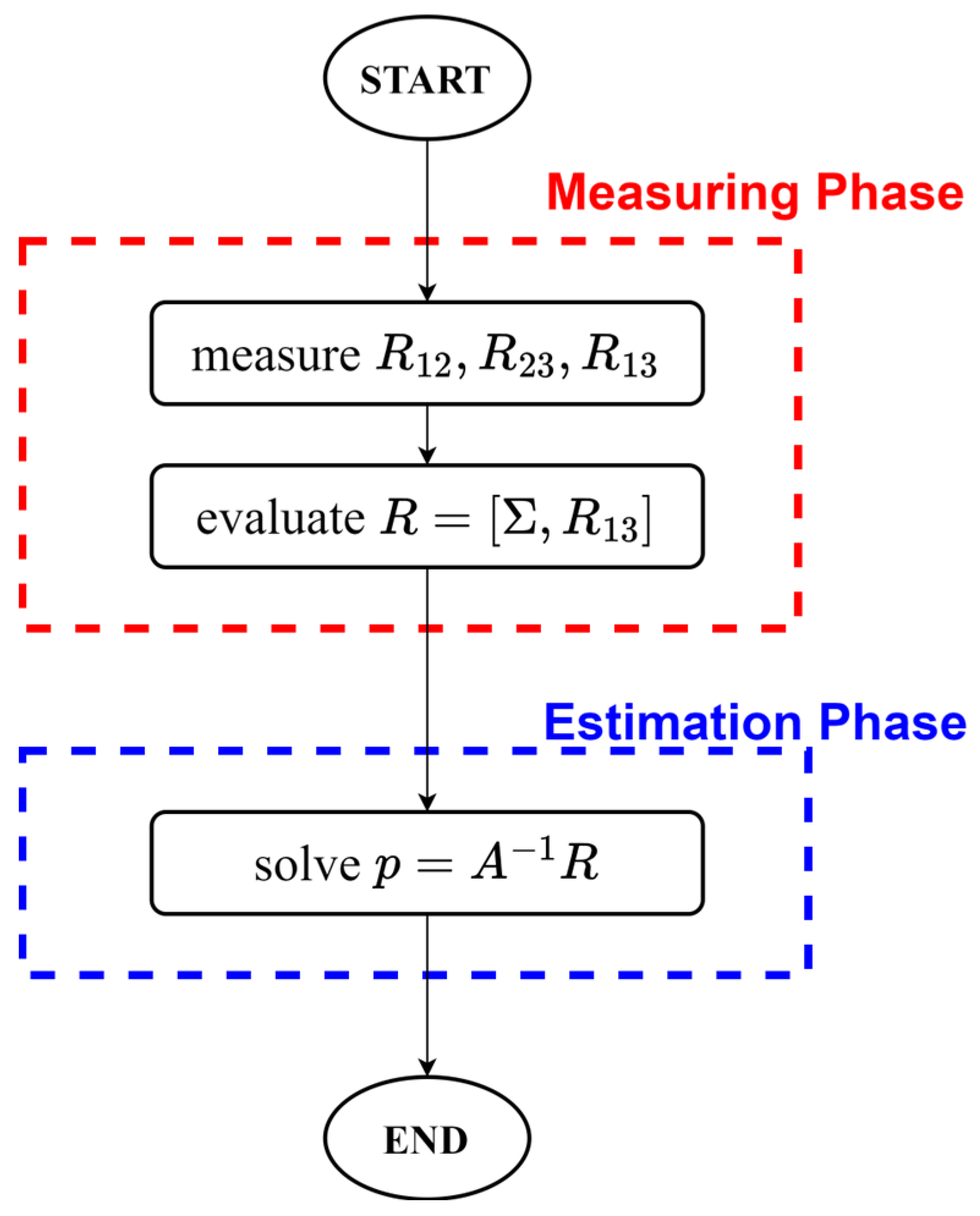
As illustrated in the flow chart of Figure 2, the estimation method can be divided into two phases. In the first phase, denoted as the measuring phase, the resistance set represented by the three-component vector S_R = [R₁₂, R₂₃, R₁₃] measured at an unknown cursor position x is used to evaluate the resistance vector R = [Σ, R₁₃]. In the second phase, denoted as the estimation phase, the previously evaluated R is used to compute p as reported in Equation (7b).

In the proposed method, each resistance set S_R, measured at an unknown position x, is used to derive a correspondent estimation of p. The estimated parameters reflect the sensor local conditions at the unknown position x where S_R is measured. This provides indirect indications of possible nonhomogeneities.

As an alternative, p can be computed using the average of N resistance sets S_R measured in N different cursor positions. Provided that the N positions are sufficiently spread, this results in spatial averaging along the resistive track with a correspondent reduction the residual dependence of $\mathit{p}$ on the cursor position x.

In this work, the parameters $\mathit{p}$ are estimated starting from each single resistance set S_R, i.e., N = 1. This offers the advantage of maintaining a biunivocal correspondence between p and the position x without introducing spatial averaging.

Since the parameters p are estimated starting from the direct measurement of the resistances R₁₂, R₂₃, and R₁₃, the lower the measurement uncertainty of the resistance measurement, the better the parameter estimation will be. The uncertainties u_c(R_c) and u_c(ξ) resulting from the resistance uncertainties u(R₁₂), u(R₁₂), and u(R₁₃) can be considered in defining a fault detection method that is robust with respect to measured data. From Equation (7b), the composite uncertainties u_c(R_c) and u_c(ξ) are given by the following:

$$u_c\left(R_c\right)=\sqrt{\frac{1}{4}{u}^2\left(R_{12}\right)+\frac{1}{4}{u}^2\left(R_{23}\right)+\frac{1}{4}{u}^2\left(R_{13}\right)}$$

(8)

$$u_c\left(\xi \right)=\sqrt{\frac{1}{L^2}{u}^2\left(R_{13}\right)}$$

(9)

2.3. Cursor Position Estimation and Compensation

There are several methods to obtain the cursor position of a resistive displacement sensor. Considering the schematization of a generic resistive displacement sensor of Figure 1a, one common method involves exciting the sensor with a known constant voltage at the terminal pair (1, 3) while reading at high-input impedance the voltage divider output at the terminal pair (2, 3), which varies as a function of the cursor position x. This method does not account for the sensor conditions represented by parameters p. Actually, the reading is to first order independent from p as long as ξ is uniform along the sensor stroke L. As no information on the sensor conditions is extracted, sensor faults cannot be anticipated nor predicted.

On the other hand, the resistances R₁₂ and R₂₃ depend on both the cursor position x at which they are measured and the parameters p. By manipulating Equations (3) and (4), the actual cursor position x can be expressed as follows:

x = (R₁₂ − R₂₃)/2ξ + L/2

(10)

An estimated cursor position x’ can be derived from Equation (10) by employing the current parameter estimates p_c = [R_cc, ξ_c]. The closer the match between p_c and p, the lower the difference will be between x’ and x. The position estimation error e_pos due to the difference between the actual unknown ξ and its current estimation ξ_c is as follows:

$$e_{\mathrm{p}\mathrm{o}\mathrm{s}}=x\prime -x=\frac{R_{12}-R_{23}}{2}\left(\frac{\xi -{\xi }_{\mathrm{c}}}{{\xi }_{\mathrm{c}}\xi }\right)$$

(11)

where R₁₂ and R₂₃ are the resistances measured in the current sensor conditions. Since the parameters vary as the sensor conditions change, it is crucial that the current parameters p_c are continuously updated since x’ depends on ξ_c.

If instead of p_c the nominal parameters p₀ = [R_c0, ξ₀] relative to an undamaged sensor are used as estimates of p during the sensor life, the estimated position $x_0\prime$ is subject to an estimation error e_pos0 given by the following:

$$e_{\mathrm{p}\mathrm{o}\mathrm{s}0}=x_0^{\prime }-x=\left(x_0^{\prime }-x^{\prime }\right)+\left(x^{\prime }-x\right)=\frac{R_{12}-R_{23}}{2}\left(\frac{{\xi }_{\mathrm{c}}-{\xi }_0}{{\xi }_{\mathrm{c}}{\xi }_0}\right)+e_{\mathrm{p}\mathrm{o}\mathrm{s}}=\delta +e_{\mathrm{p}\mathrm{o}\mathrm{s}}$$

(12)

The position estimation error e_pos0 can be seen as the sum of e_pos given by Equation (11) and an additive error $\delta$ related to the difference between the current parameter ξ_c and ξ₀ employed for estimating position.

The additive error δ is zero when ξ_c = ξ₀, i.e., when ξ does not vary from the undamaged conditions. It also shows that the error is higher the farther the cursor is from L/2. As the position error e_pos does not depend on R_c as long as R_c is finite and Equation (11) remains valid, the proposed estimation method is unaffected by R_c.

Starting from Equation (12), if the estimate of ξ is constantly updated, the position estimation error e_pos0 can be reduced to e_pos by nulling the additive position estimation error δ. In this perspective, the method proposed to reduce the position estimation error can be seen as a self-compensation method.

2.4. Fault Detection

The parameters R_c and ξ are known to play a crucial role in defining the conditions of the resistive displacement sensor as they are directly affected by sensor wearout and faults [23]. Therefore, the proposed fault detection method focuses on assessing progressive sensor wearout or sudden failure by comparing the variation in R_c and ξ with reference values by means of alarm thresholds. Innovatively, this approach is built on a model that allows determination of the sensor conditions during its operation, without disconnecting it from the host system and without requiring knowledge of the cursor position x.

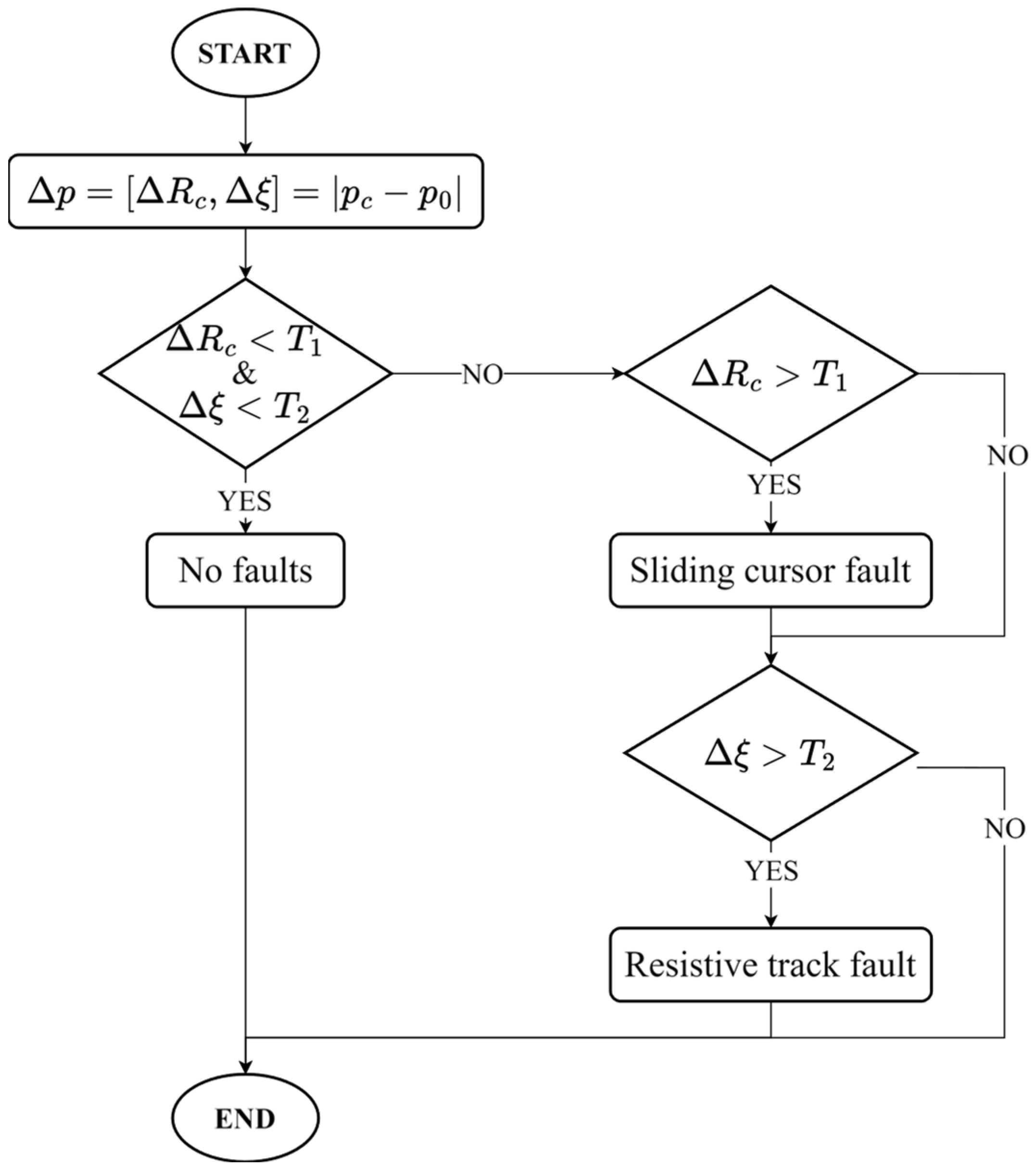
As illustrated in the flow chart of Figure 3, faults are detected on the basis of parameter variations Δp = [ΔR_c, Δξ] = |p_c − p₀|, where p_c = [R_cc, ξ_c] and p₀ = [R_c0, ξ₀] represent the sensor parameters in the current and initial undamaged conditions, respectively. The nominal parameters p₀ are calculated as the spatial average of the initial parameters R_c and ξ estimated along the entire sensor stroke. The parameters p₀ could be determined during factory calibration or directly in the field, during the first installation. It is expected that R_c and ξ variations are mostly related to sliding cursor and resistive track faults, respectively.

Fault detection is based on threshold surpassing. Specifically, if both ΔR_c and Δξ are lower than their respective alarm thresholds T₁ and T₂, then no fault is detected. Differently, the sensor is faulty, and the fault could affect the resistive track, the sliding cursor, or both depending on which threshold is surpassed.

The thresholds T₁ and T₂ can be set empirically on the basis of ensemble standard deviations σ(R_c0) and σ(ξ₀) derived from a suitably large population representative of undamaged sensors, or from each individual sensor at the installation time in the field. Assuming that model parameters for an undamaged sensor are random variables with normal distribution, it is reasonable to suppose that changes that exceed the range of ±3σ(R_c0) and ±3σ(ξ₀) are ascribable to an occurred alteration in the sensor conditions due to wearout or fault.

3. Results

The sensor model, along with the parameter estimation, the self-compensation, and the fault detection methods have been simulated and experimentally tested.

The simulations have estimated the parameters from a set of resistance values corrupted with pseudorandom numerical noise, while in the experimental tests the parameters have been derived from measurements on a Device Under Test (DUT), i.e., a resistive displacement sensor, placed in two different conditions, namely undamaged and faulty.

The term undamaged here refers to a sensor that has never been used and has been stored in compliance with the requirements described in the sensor datasheet. Instead, the term faulty here indicates a sensor subject to a resistive track and sliding cursor wearout, where the resistive track wear along x is virtually uniform. Wear has been considered among the failures listed in Section 2.1 as it represents the main and most common failure mode.

The simulations have been aimed at evaluating the parameter estimation variability with respect to the measurement accuracy of resistances R₁₂, R₂₃, and R₁₃. The experimental tests have been aimed at assessing the fitting accuracy of the sensor model defined as the difference between the measured resistances R₁₂, R₂₃, and R₁₃ and those synthetized from the sensor model. Furthermore, the estimated parameters have been employed to evaluate the self-compensation method in reducing the position estimation error and the effectiveness of alarm thresholds T₁ and T₂ in detecting wear failure.

3.1. Simulation Results

Simulations have been performed in MATLAB 2022b to repeatedly estimate the model parameters R_c and ξ from a set of resistances R₁₂, R₂₃, and R₁₃ corrupted with numerical noise. The parameter mean values μ and standard deviations σ have been calculated from the estimates across the repetitions taken at different positions.

The resistances R₁₂, R₂₃, and R₁₃ forming the resistance set S_R have been synthetized from their respective analytical expressions reported in Equations (3)–(5), fixing the ideal parameters $\overline{\mathit{p}}$ = $\left[\overline{R_c},\overline{\xi }\right]$ = [100 Ω; 50,000 Ω/m], the sensor stroke L = 100 mm and sweeping the displacement from x = 0 to x = L with a step of 1 mm. The values chosen for $\overline{\mathit{p}}$ are representative of the actual sensor that has been experimentally tested as detailed in Section 3.2. In particular, $\overline{R_c}$ = 100 Ω includes non-idealities like the conductive track resistance and the resistance of the connecting terminals. A normally distributed pseudorandom numerical noise with a standard deviation σ_n = 1 Ω has been added to corrupt R₁₂, R₂₃, and R₁₃.

For each considered cursor position x, the parameters have been estimated from the corresponding resistance set S_R. Then, the mean values μ and standard deviations σ with respect to x have been calculated from the estimates. The obtained results are reported in

Table 2. Parameter estimation errors and standard deviations σ obtained by ranging x from 0 to L with a 1 mm step (M = 100 parameter estimations), assuming as a reference the ideal parameters $\overline{\mathit{p}}$ = $\left[\overline{R_c},\overline{\xi }\right]$ = [100 Ω; 50,000 Ω/m]. The uncertainties of the parameter mean values μ and standard deviations σ are derived from the parameter composite uncertainties u_c(R_c) and u_c(ξ).

${\mathit{R}}_{\mathbf{c}} \mathbf{Estimation} \mathbf{Error} \overline{{\mathit{R}}_{\mathit{c}}}-\mathsf{\mu }\left({\mathit{R}}_{\mathit{c}}\right)$$\left[\mathsf{\Omega }\right]$	${\mathit{R}}_{\mathbf{c}} \mathbf{Standard} \mathbf{Deviation} \mathsf{\sigma }\left({\mathit{R}}_{\mathit{c}}\right)$$\left[\mathsf{\Omega }\right]$	$\mathsf{\xi } \mathbf{Estimation} \mathbf{Error} \overline{\mathsf{\xi }}-\mathsf{\mu }\left(\mathsf{\xi }\right)[\mathsf{\Omega }/\mathbf{m}]$	$\mathsf{\xi } \mathbf{Standard} \mathbf{Deviation} \mathsf{\sigma }\left(\mathsf{\xi }\right)$$[\mathsf{\Omega }/\mathbf{m}]$
0.1 ± 0.1	0.8 ± 0.1	−1 ± 1	11.5 ± 0.7

as the difference between $\overline{\mathit{p}}$ and the estimated parameter mean values μ, along with their standard deviations σ. Figure 4 and Figure 5 report the parameter estimation errors as a function of the position along the sensor stroke.

The simulation evaluates the variability of estimated parameters with respect to the measurement accuracy of resistances R₁₂, R₂₃, and R₁₃. The parameter estimation is adequate for the application scope because the percentage deviations between the ideal parameters $\overline{\mathit{p}}$ and the mean values of the estimated parameters are less than ±0.1%. Furthermore, the parameter standard deviations σ(R_c) and σ(ξ) agree with the corresponding composite uncertainties u_c(R_c) = $\sqrt{3}$/2 Ω and u_c(ξ) = 10 Ω/m, obtained from Equations (8) and (9) by setting u(R₁₂) = u(R₂₃) = u(R₁₃) = σ_n = 1 Ω.

3.2. Experimental Setup

The DUT is a resistive linear displacement sensor (Gefran PK), with a displacement full-scale span (FSS) L = 100 mm, a nominal resistive track resistance of 5 kΩ and an independent linearity error of ±0.05% FSS.

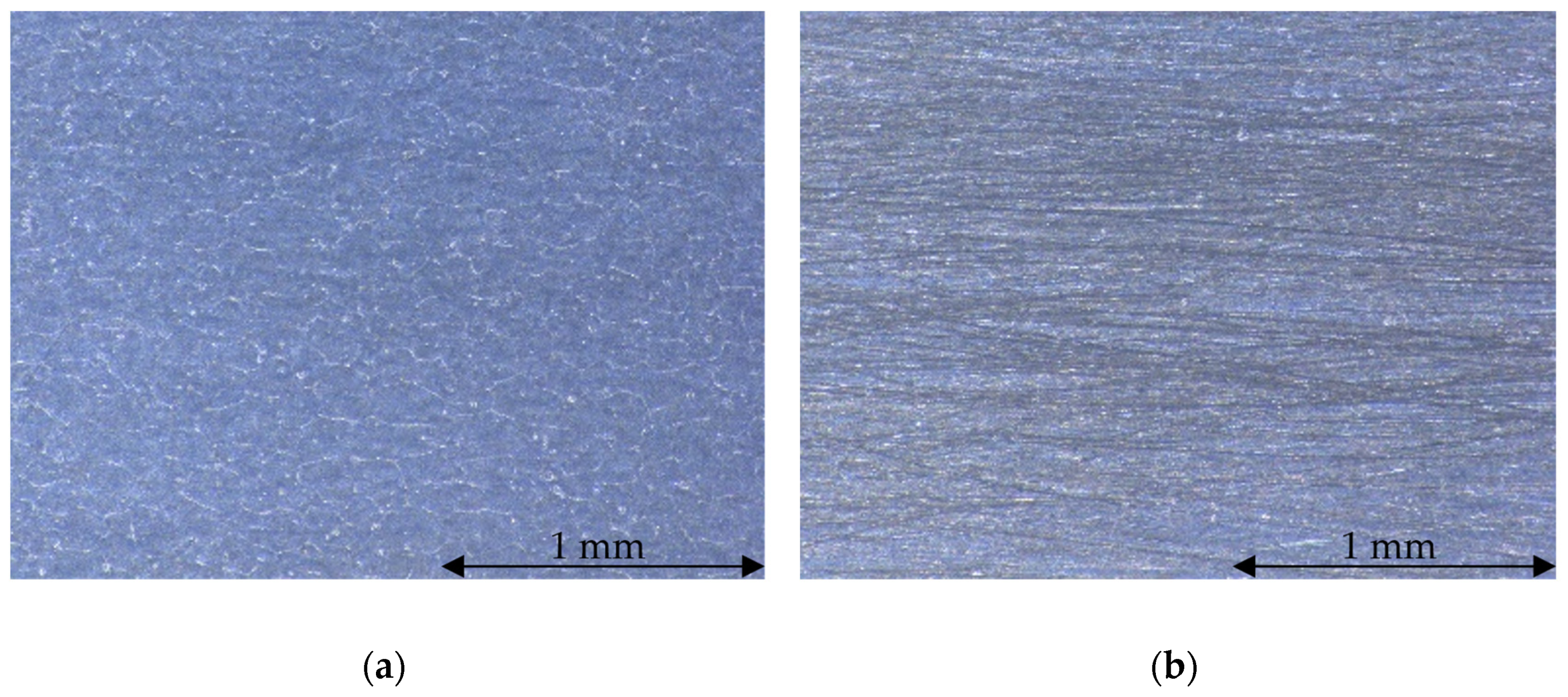
Sensor wearout has been intentionally provoked by sliding the cursor back and forth throughout the whole sensor stroke for 10⁶ cycles. Figure 6 shows the stress-test machine adopted to induce wear, while Figure 7 shows the wearout effect produced on the resistive track.

The assembled experimental setup comprises a linear positioning stage, a digital multimeter, and a personal computer, as shown in Figure 8 and Figure 9.

The sensor parameters are estimated from the resistance sets S_R measured in M different cursor positions along the sensor stroke. Resistances have been measured by means of a 6.5-digit digital multimeter (Keithley DAQ6510, Cleveland, OH, USA) equipped with a multiplexer module (Keithley 7700), providing a specified resistance measurement accuracy u(R) = 1 Ω in the 10 kΩ range of interest.

The sensor cursor displacement has been set by a precision linear positioning stage (Physik Instrumente LS-270, Karlsruhe, Germany) with a calibrated position accuracy in the order of ±1 µm. A LabVIEW script has been developed to implement the parameter estimation method and handle the experimental setup. The script is designed to move the linear stage to M different positions and trigger the digital multimeter to measure the components of S_R at each position.

3.3. Experimental Results

Experimental tests have been carried out to estimate the parameters of an undamaged (U) sensor and a faulty (F) sensor, denoted as p_u = [R_cu, ξ_u] and p_f = [R_cf, ξ_f], respectively. For the undamaged and faulty sensors, the respective resistance sets S_Ru and S_Rf have been repeatedly measured M times for the position x ranging from 0 to L with a 1 mm step resulting in M = 100, as schematized in Figure 10. From each set S_Ru and S_Rf, the parameters p_u and p_f have been estimated according to Equation (7b).

Table 3. Parameter mean values μ and standard deviations σ, along with the RMSE of the residuals r₁₂, r₂₃ and r₁₃ obtained in the experimental test. Parameter estimations are performed from the resistance sets S_R measured M = 100 times for x ranging from 0 to L with a 1 mm step. Since the resistance measurement uncertainty is u(R) = 1 Ω, the parameter composite uncertainties are u_c(R_c) = 0.9 Ω and u_c(ξ) = 10 Ω/m. The uncertainties of the parameter mean values μ, standard deviations σ, and RMSE of the residuals r₁₂, r₂₃ and r₁₃ are derived from u_c(R_c), u_c(ξ), and u(R).

Sensor Condition	Rc Mean Value $\mathsf{\mu }\left({\mathit{R}}_{\mathbf{c}}\right)$$\left[\mathsf{\Omega }\right]$	${\mathit{R}}_{\mathbf{c}} \mathbf{Standard} \mathbf{Deviation} \mathsf{\sigma }\left({\mathit{R}}_{\mathbf{c}}\right)$$\left[\mathsf{\Omega }\right]$	$\mathsf{\xi } \mathbf{Mean} \mathbf{Value} \mathsf{\mu }\left(\mathsf{\xi }\right)$$\left[\mathsf{\Omega }/\mathbf{m}\right]$	$\mathsf{\xi } \mathbf{Standard} \mathbf{Deviation} \mathsf{\sigma }\left(\mathsf{\xi }\right)$$\left[\mathsf{\Omega }/\mathbf{m}\right]$	${\mathbf{r}}_{12}$$\mathbf{Root} \mathbf{Mean} \mathbf{Square} \mathbf{Error} \mathbf{R}\mathbf{M}\mathbf{S}\mathbf{E}\left({\mathbf{r}}_{12}\right)$$\left[\mathsf{\Omega }\right]$	${\mathbf{r}}_{23}$$\mathbf{Root} \mathbf{Mean} \mathbf{Square} \mathbf{Error} \mathbf{R}\mathbf{M}\mathbf{S}\mathbf{E}\left({\mathbf{r}}_{23}\right)$$\left[\mathsf{\Omega }\right]$	${\mathbf{r}}_{13}$$\mathbf{Root} \mathbf{Mean} \mathbf{Square} \mathbf{Error} \mathbf{R}\mathbf{M}\mathbf{S}\mathbf{E}\left({\mathbf{r}}_{13}\right)$$\left[\mathsf{\Omega }\right]$
Undamaged (U)	123.0 ±0.1	4.5 ± 0.1	49,058 ± 1	1.3 ± 0.7	10.9 ± 0.1	10.9 ± 0.1	0.1 ± 0.1
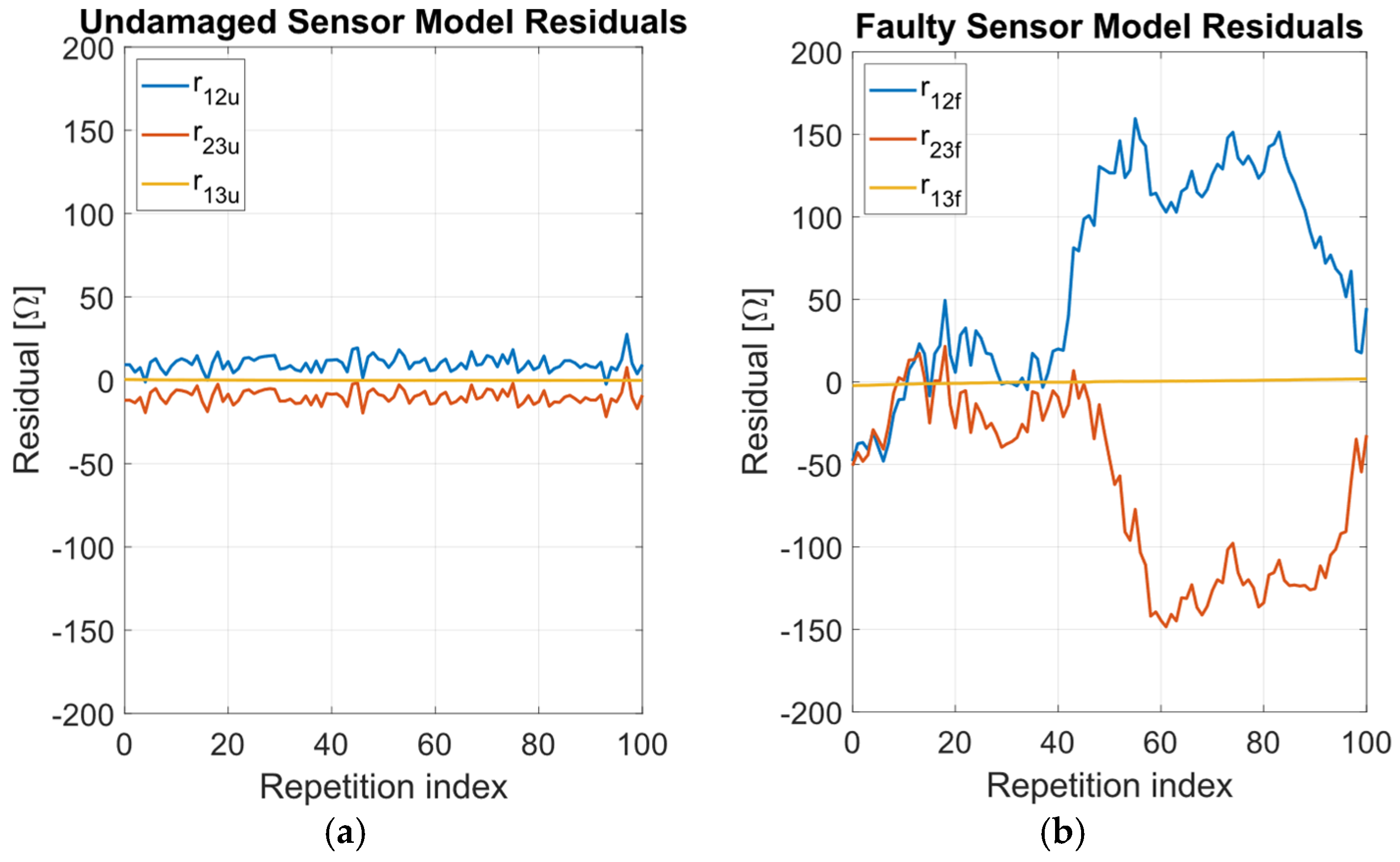
Faulty (F)	161.6 ± 0.1	21.9 ± 0.1	62,142 ± 1	9.9 ± 0.7	88.6 ± 0.1	83.1 ± 0.1	1.1 ± 0.1

reports the mean values P_u = [μ(R_cu), μ(ξ_u)] and P_f = [μ(R_cf), μ(ξ_f)], and standard deviations σ_u = [σ(R_cu), σ(ξ_u)] and σ_f = [σ(R_cf), σ(ξ_f)] for p_u and p_f obtained over the M repetitions at varying x. From P_u and P_f inserted into Equations (3)–(5), the terms R_mu = [R_12mu, R_23mu, R_13mu] and R_mf = [R_12mf, R_23mf, R_13mf] have been obtained, where the subscript m indicates outcomes from the model. Hence the model residuals have been computed for the undamaged and faulty sensor as r_u = [r_12u, r_23u, r_13u] = S_Ru − R_mu and r_f = [r_12f, r_23f, r_13f] = S_Rf − R_mf, respectively. The residuals r_u and r_f have been evaluated for all the M repetitions at which S_Ru and S_Rf have been measured. The root mean square errors (RMSE) of the residuals are also reported in Table 3. Figure 11 shows the estimated parameters p_u and p_f while Figure 12a,b report the residuals r_u and r_f as a function of repetition index ranging from 1 to M = 100.

The position estimation error e_pos is evaluated for both the U and F sensors, for all the cursor positions at which S_Ru and S_Rf are measured. The true, i.e., actual, cursor position x is assumed to be given by the linear positioning stage taken as the reference. The position estimations x’ are derived from Equation (10) by employing μ(ξ_u) and μ(ξ_f) for the U and F sensor, respectively. Figure 13 shows the position estimation error e_pos for both the U and F sensors as a function of x. Figure 14 shows e_pos obtained for the faulty sensor both with and without the application of the self-compensation method described in Section 2.3, where the uncompensated cursor positions are intentionally estimated using μ(ξ_u) in order to simulate a mismatch between the nominal, i.e., initial, and the current sensor conditions.

Lastly, the fault detection method discriminates the fault and no-fault conditions on the basis of the parameter variations Δp_u = |p_u − P_u| and Δp_f = |p_f − P_u|. The fault detection thresholds T₁ and T₂ have been set based on the p_u standard deviations σ_u, resulting in T₁ = 3σ(R_cu) = 13.5 Ω and T₂ = 3σ(ξ_u) = 3.9 Ω/m.

4. Discussion

Considering the simulation results described in Section 3.1, the normally distributed pseudorandom numerical noise added to R₁₂, R₂₃, and R₁₃ and the resulting parameter variability are reflected in the parameter composite uncertainties u_c(ξ) and u_c(R_c) expressed in Equations (8) and (9). Assuming the resistance uncertainties equal to the noise standard deviation, i.e., u(R₁₂) = u(R₂₃) = u(R₁₃) = σ_n = 1 Ω, the parameter composite uncertainties result u_c(R_c) = $\sqrt{3}$/2 Ω and u_c(ξ) = 10 Ω/m., which agree with the simulation results σ(R_c) = 0.8 Ω and σ(ξ)=11 Ω/m.

The standard deviations of the parameters R_c and ξ can be analyzed to compare the variability of the parameters obtained in the simulations with those from experimental results. Although the noise standard deviation σ_n in simulations is taken equal to the resistance measurement uncertainty u(R), i.e., u(R) = σ_n = 1 Ω, the experimental standard deviations of R_c, σ(R_cu) = 4.5 Ω and σ(R_cf) = 21.9 Ω, are larger than σ(R_c) = 0.8 Ω for simulations.

This is consistent with the fact that σ(R_cu) and σ(R_cf) cannot be imputed exclusively to u(R), in fact they can be ascribed to the nonideality of R₁₂ and R₂₃ trends as a function of x due to the presence of faults, described by the residuals r₁₂ and r₂₃. Similarly, the residual r₁₃ explains the difference between the experimental standard deviations σ(ξ_u) = 1.3 Ω and σ(ξ_f) = 9.9 Ω with the simulated one σ(ξ) = 11.5 Ω.

Considering the experimental results described in Section 3.3, Figure 11 shows a visible dependence of R_cf on the repetition index and, in turn, versus position x. Such dependence shows nonuniform variations along the resistive track length L, with regions where the contact resistance between the sliding cursor and the resistive track is higher. The microscope analysis confirms that the regions where the contact resistance is higher match with the regions where the resistive track is mostly worn. Therefore, the proposed method theoretically allows detection of local faults through R_c trend analysis.

The sensor model goodness of fit is evaluated on the basis of the residuals r_u and r_f. As shown in Figure 12a,b, for the undamaged sensor the RMSEs of r_u are $~$0.2% of the resistive track nominal resistance, which is adequately low for fault detection and estimation of position x’. For the faulty sensor, the RMSEs of r_f increase compared to the undamaged case due to the trends of R₁₂ and R₂₃ as a function of x caused by nonhomogeneous resistive track wear along its length.

As shown in Figure 13, the position estimation error e_pos for the undamaged sensor is approximately constant throughout the sensor stroke, with a mean value of 0.2 mm. For the faulty sensor, e_pos is an order of magnitude higher spanning a range of roughly 2 mm. As reported in Figure 14, the self-compensation method successfully reduces e_pos to a span of about 2 mm in the faulty case versus the value of 30 mm obtained intentionally using μ(ξ_u) to represent the case when the parameter estimates are not updated to the current values.

Given the chosen thresholds T₁ = 3σ(R_cu) and T₂ = 3σ(ξ_u), the results obtained in applying the fault detection method are shown in the confusion matrices of Figure 15.

The fault detection method has been evaluated using accuracy, precision, and recall performance metrics. Accuracy measures the fault detection correctness, precision evaluates the number of actual faults identified, while recall assesses the effectiveness in detecting faults among all instances of faults. The performance metrics obtained for the resistive track and sliding cursor fault detections are reported in

Table 4. Accuracy, precision and recall performance metrics for the sliding cursor and resistive track fault detections. Accuracy = (TP + TN)/(TP + TN + FP + FN), precision = TP/(TP + FP), and recall = TP/(TP + FN), where TP, TN, FP, and FN are the true positive, true negative, false positive, and false negative fault predictions, respectively.

Type of Fault Detected	Accuracy	Precision	Recall
Sliding Cursor	95.5%	98.9%	92.0
Resistive Track	99.0%	98.0%	100%

.

The false negative sliding cursor fault detections are due to the variability of R_c as a function of x caused by nonhomogeneous wear of the resistive track. A possible solution could be acting on threshold values. For example, lowering T₁ to equal σ(R_cu) results in the sliding cursor fault detection recall increasing to 96.0%. However, threshold lowering makes the fault detection method more prone to false positives, leading the precision to drop to 78.6%.

Moreover, the uncertainty of the standard deviations of the parameters in the thresholds T₁ and T₂ has an impact on the accuracy and precision metrics for resistive track fault detection. In particular, accuracy and precision vary within [97.5%; 100%] and [95.2%; 100%], respectively.

5. Conclusions

This work introduces a suitably general model for resistive displacement sensors and proposes thereof an innovative fault detection method that can be applied with the sensor in operation providing self-diagnostic capabilities. Based on the output of the self-diagnostic step, a self-compensation method with automatic updating is in turn derived to increase the accuracy in sensors subject to progressive wearout. The proposed model and methods have been validated by both numerical simulations and experimental tests on real devices.

The position is estimated by exploiting the sensor model and the initial value of ξ. The self-compensation method reduces the position estimation error by considering the difference between the current and initial values of ξ, which causes a position estimation error. The self-compensation method successfully reduces the position estimation error e_pos in the faulty case, intentionally obtained using μ(ξ_u), from a span of 30 mm to a span of 2 mm. The proposed fault detection method evaluates the progressive sensor wearout or sudden failure by comparing the variation in the current parameters R_c and ξ with respect to their initial values against the alarm thresholds T₁ and T₂, respectively. The fault detection method, for T₁ = 3σ(R_cu) and T₂ = 3σ(ξ_u), has shown a resistive track and sliding cursor fault detection accuracy of 99.0% and 95.5%, respectively. Lowering T₁ from 3σ(R_cu) to σ(R_cu) has increased the sliding cursor fault detection recall to 96.0%, involving the precision to drop to 78.6% as the threshold lowering makes the fault detection method more prone to false positives.

The future work will involve the implementation of the proposed methods and their testing in a dynamic industrial process.

6. Patents

There is a patent application resulting from the work reported in this manuscript [26].

References

- Valenzuela, R.; Vazquez, M.; Hernando, A. A Position Sensor Based on Magnetoimpedance. J. Appl. Phys. 1996, 79, 6549–6551. [Google Scholar] [CrossRef]
- Aiestaran, P.; Dominguez, V.; Arrue, J.; Zubia, J. A Fluorescent Linear Optical Fiber Position Sensor. Opt. Mater. 2009, 31, 1101–1104. [Google Scholar] [CrossRef]
- Nagaoka, T.; Uchiyama, A. Development of a Small Wireless Position Sensor for Medical Capsule Devices. In Proceedings of the 26th Annual International Conference of the IEEE Engineering in Medicine and Biology Society, San Francisco, CA, USA, 1–5 September 2004; Volume 1, pp. 2137–2140. [Google Scholar]
- Bebek, O.; Cavusoglu, C.M. Whisker-like Position Sensor for Measuring Physiological Motion. IEEE/ASME Trans. Mechatron. 2008, 13, 538–547. [Google Scholar] [CrossRef]
- Datlinger, C.; Hirz, M. Benchmark of Rotor Position Sensor Technologies for Application in Automotive Electric Drive Trains. Electronics 2020, 9, 1063. [Google Scholar] [CrossRef]
- Kirchhoff, M.R.; Boese, C.; Güttler, J.; Feldmann, M.; Büttgenbach, S. Innovative High-Precision Position Sensor Systems for Robotic and Automotive Applications. Procedia Chem. 2009, 1, 501–504. [Google Scholar] [CrossRef]
- Reininger, T.; Welker, F.; von Zeppelin, M. Sensors in Position Control Applications for Industrial Automation. Sens. Actuators A Phys. 2006, 129, 270–274. [Google Scholar] [CrossRef]
- Zhu, M.; Li, J.; Wang, W.; Chen, D. Self-Detection and Self-Diagnosis Methods for Sensors in Intelligent Integrated Sensing System. IEEE Sens. J. 2021, 21, 19247–19254. [Google Scholar] [CrossRef]
- Basri, E.I.; Abdul Razak, I.H.; Ab-Samat, H.; Kamaruddin, S. Preventive Maintenance (PM) Planning: A Review. J. Qual. Maint. Eng. 2017, 23, 114–143. [Google Scholar] [CrossRef]
- Betta, G.; Pietrosanto, A. Instrument Fault Detection and Isolation: State of the Art and New Research Trends. IEEE Trans. Instrum. Meas. 2000, 49, 100–107. [Google Scholar] [CrossRef]
- Isermann, R. Model-Based Fault-Detection and Diagnosis—Status and Applications. Annu. Rev. Control 2005, 29, 71–85. [Google Scholar] [CrossRef]
- Samy, I.; Postlethwaite, I.; Gu, D.-W. Survey and Application of Sensor Fault Detection and Isolation Schemes. Control Eng. Pract. 2011, 19, 658–674. [Google Scholar] [CrossRef]
- Thirumarimurugan, M.; Bagyalakshmi, N.; Paarkavi, P. Comparison of Fault Detection and Isolation Methods: A Review. In Proceedings of the 10th International Conference on Intelligent Systems and Control, ISCO 2016, Coimbatore, India, 7–8 January 2016; Institute of Electrical and Electronics Engineers Inc.: Piscataway, NJ, USA, 2016; pp. 1–6. [Google Scholar]
- Lou, X.; Willsky, A.S.; Verghese, G.C. Optimally Robust Redundancy Relations for Failure Detection in Uncertain Systems. Automatica 1986, 22, 333–344. [Google Scholar] [CrossRef]
- Clark, R.N.; Fosth, D.C.; Walton, V.M. Detecting Instrument Malfunctions in Control Systems. IEEE Trans. Aerosp. Electron. Syst. 1975; AES-11, 465–473. [Google Scholar] [CrossRef]
- Willsky, A.S.; Deyst, J.J.; Crawford, B.S. Adaptive Filtering and Self-Test Methods for Failure Detection and Compensation. In Proceedings of the Joint Automatic Control Conference, Austin, TX, USA, 18–21 June 1974; pp. 637–645. [Google Scholar]
- Mohapatra, D.; Subudhi, B.; Daniel, R. Real-Time Sensor Fault Detection in Tokamak Using Different Machine Learning Algorithms. Fusion Eng. Des. 2020, 151, 111401. [Google Scholar] [CrossRef]
- Warriach, E.U.; Tei, K. Fault Detection in Wireless Sensor Networks: A Machine Learning Approach. In Proceedings of the 16th IEEE International Conference on Computational Science and Engineering, CSE 2013, Sydney, NSW, Australia, 3–5 December 2013; pp. 758–765. [Google Scholar]
- Jan, S.U.; Lee, Y.D.; Koo, I.S. A Distributed Sensor-Fault Detection and Diagnosis Framework Using Machine Learning. Inf. Sci. 2021, 547, 777–796. [Google Scholar] [CrossRef]
- Henry, M.P.; Clarke, D.W. The Self-Validating Sensor: Rationale, Definitions and Examples. Control Eng. Pract. 1993, 1, 585–610. [Google Scholar] [CrossRef]
- Çinar, Z.M.; Nuhu, A.A.; Zeeshan, Q.; Korhan, O.; Asmael, M.; Safaei, B. Machine Learning in Predictive Maintenance towards Sustainable Smart Manufacturing in Industry 4.0. Sustainability 2020, 12, 8211. [Google Scholar] [CrossRef]
- Mazzoli, F.; Alghisi, D.; Ferrari, V. Self-Diagnostic Method for Resistive Displacement Sensors. Proceedings 2024, 97, 164. [Google Scholar] [CrossRef]
- Saitoh, M.; Osada, K. Long Life Potentiometric Position Sensor—Its Material and Application. SAE Trans. 1991, 100, 251–262. [Google Scholar]
- Hattangadi, A.A. Potentiometer Failures. In Failure Prevention of Plant and Machinery; McGraw-Hill Education: New York, NY, USA, 2004; ISBN 9780070483095. [Google Scholar]
- Todd, C.D. The Potentiometer Handbook: Users’ Guide to Cost-Effective Applications; McGraw-Hill: New York, NY, USA, 1975; ISBN 978-0070066908. [Google Scholar]
- Mazzoli, F.; Alghisi, D.; Ferrari, V. Position Sensor Configured to Monitor the Condition and/or the Wear Level of That Position Sensor During Its Use.
Figure 1.
(a) Schematization of a generic resistive linear displacement sensor with (b) the corresponding resistive circuit modeling.
Figure 2.
Parameter estimation method flow chart.
Figure 3.
Fault detection method flow chart.
Figure 4.
Estimation error of the parameter Rc versus the position x along the sensor stroke.
Figure 5.
Estimation error of the parameter ξ versus the position x along the sensor stroke.
Figure 6.
Stress-test machine employed to induce wearout in the resistive track and sliding cursor.
Figure 7.
Images obtained with a digital microscopy system (Leica DMS300) of the undamaged (a) and wearout (b) resistive track.
Figure 8.
Block diagram of the adopted experimental setup.
Figure 9.
Photo of the assembled experimental setup.
Figure 10.
Schematization of SRu and SRf measurement processes. The resistance sets SRu and SRf are measured from the undamaged and faulty sensor over M repetitions taken for x varying from 0 to L with a 1 mm step.
Figure 11.
Parameters pu and pf estimated, respectively, from the measured resistance sets SRu and SRf as a function of the repetition index ranging from 1 to M = 100.
Figure 12.
Residuals ru = SRu − Rmu (a) and rf = SRf − Rmf (b) resulting from the measured SRu and SRf as a function of the repetition index ranging from 1 to M = 100.
Figure 13.
Position estimation error epos for to the undamaged (U) and faulty (F) sensors versus the actual cursor position x.
Figure 14.
Position estimation error epos for to the faulty (F) sensor, with and without the self-compensation method applied, versus the actual cursor position x. The uncompensated cursor positions have been deliberately estimated using μ(ξu) to simulate a discrepancy between the nominal and current sensor conditions.
Figure 15.
Confusion matrices for the sliding cursor and resistive track fault detections.