


DEMA: A Deep Learning-Enabled Model for Non-Invasive Human Vital Signs Monitoring Based on Optical Fiber Sensing


Abstract
1. Introduction
1.1. Background
1.2. Progress of Research at the Current Stage
2. Methodology
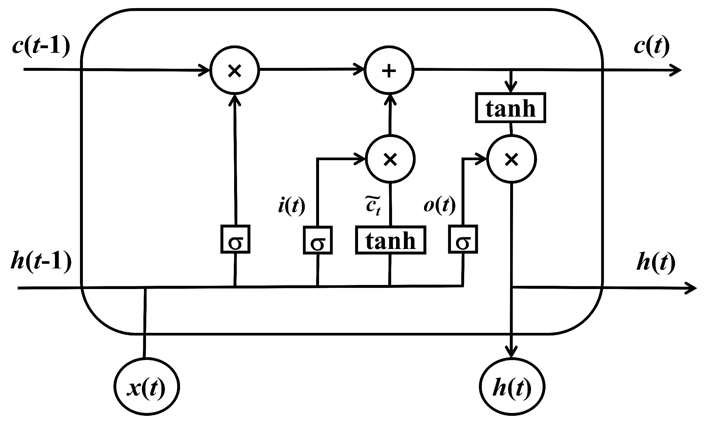
2.1. RNN and LSTM in Time-Series Data
2.2. EMD and LSTM Integration in Signal Processing
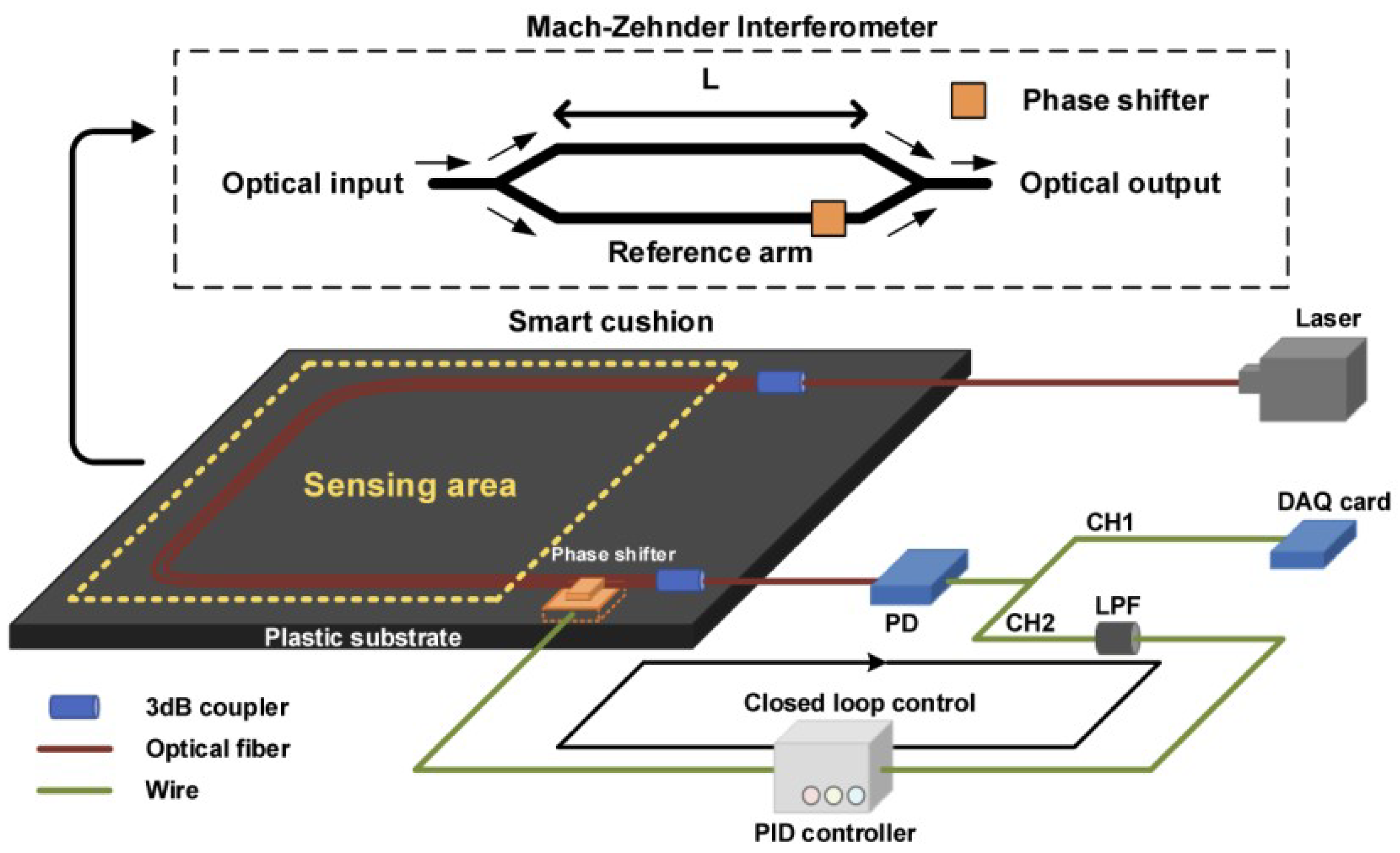
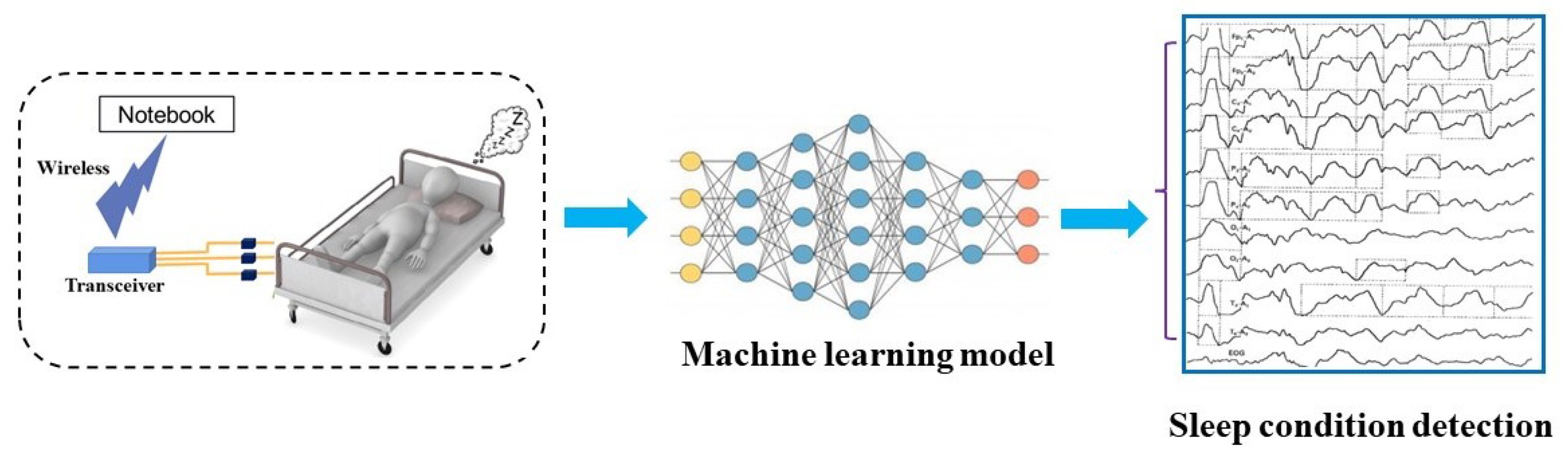
2.3. Design of Optical Fiber Monitoring
2.4. EMD Algorithm
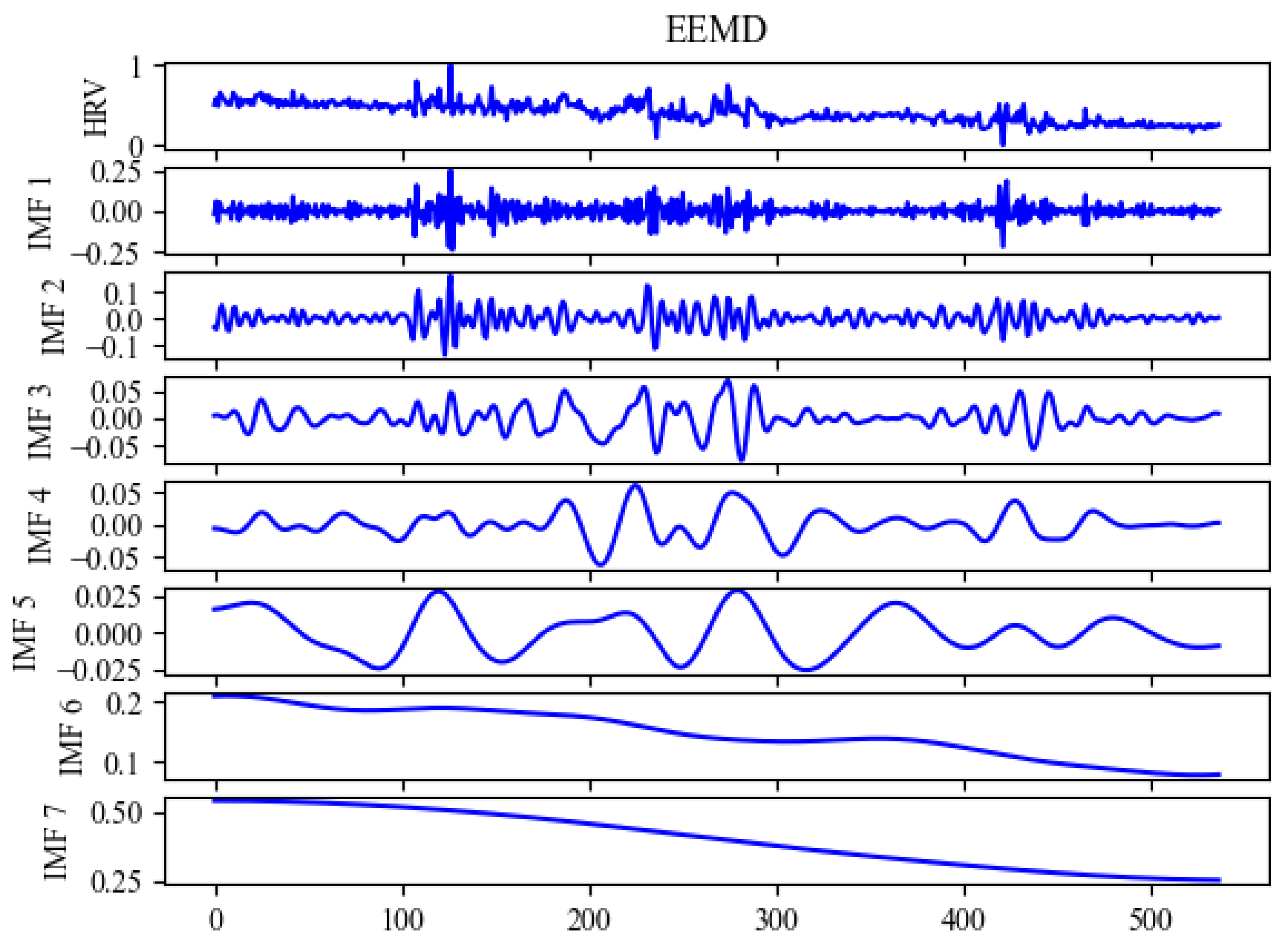
2.5. EEMD Algorithm
2.6. DEMA Algorithm
3. Experiment and Discussion
3.1. Data Resources and Processing
3.2. Experimental Preparation and Results
3.3. Summary
4. Conclusions and Future Works
4.1. Research Summary
4.2. Future Works
Author Contributions
Funding
Data Availability Statement
Conflicts of Interest
References
- Smith, I.; Mackay, J.; Fahrid, N.; Krucheck, D. Respiratory rate measurement: A comparison of methods. Br. J. Healthc. Assist. 2011, 5, 18–23. [Google Scholar] [CrossRef]
- Favilla, R.; Zuccalà, V.C.; Coppini, G. Heart rate and heart rate variability from single-channel video and ICA integration of multiple signals. IEEE J. Biomed. Health Inf. 2019, 23, 2398–2408. [Google Scholar] [CrossRef]
- Kong, W.; Dong, Z.Y.; Jia, Y.; Hill, D.J.; Xu, Y.; Zhang, Y. Short-Term Residential Load Forecasting Based on LSTM Recurrent Neural Network. IEEE Trans. Smart Grid 2019, 10, 841–851. [Google Scholar] [CrossRef]
- Wang, Q.; Zhang, Y.; Chen, G.; Chen, Z.; Hee, H.I. Assessment of heart rate and respiratory rate for perioperative infants based on ELC model. IEEE Sens. J. 2021, 21, 13685–13694. [Google Scholar] [CrossRef]
- Wang, Q.; Lyu, W.; Cheng, Z.; Yu, C. Noninvasive Measurement of Vital Signs with the Optical Fiber Sensor Based on Deep Learning. J. Light. Technol. 2023, 41, 4452–4462. [Google Scholar] [CrossRef]
- Shin, Y.-S.; Kim, J. Sensor Data Reconstruction for Dynamic Responses of Structures Using External Feedback of Recurrent Neural Network. Sensors 2023, 23, 2737. [Google Scholar] [CrossRef]
- Wang, M.; Ye, X.-W.; Jia, J.-D.; Ying, X.-H.; Ding, Y.; Zhang, D.; Sun, F. Confining Pressure Forecasting of Shield Tunnel Lining Based on GRU Model and RNN Model. Sensors 2024, 24, 866. [Google Scholar] [CrossRef] [PubMed]
- Xie, H.; Huang, Z.; Leung, F.H.F.; Ju, Y.; Zheng, Y.-P.; Ling, S.H. A Structure-Affinity Dual Attention-based Network to Segment Spine for Scoliosis Assessment. In Proceedings of the 2023 IEEE International Conference on Bioinformatics and Biomedicine (BIBM), Istanbul, Turkey, 5–8 December 2023; pp. 1567–1574. [Google Scholar] [CrossRef]
- Zhang, Q.; Wang, Q.; Lyu, W.; Yu, C. A Deep Learning-based Model for Human Non-invasive Vital Sign Signal Monitoring with Optical Fiber Sensor. In Proceedings of the 2023 Asia Communications and Photonics Conference/2023 International Photonics and Optoelectronics Meetings (ACP/POEM), Wuhan, China, 4–7 November 2023. [Google Scholar]
- İşbitirici, A.; Giarré, L.; Xu, W.; Falcone, P. LSTM-Based Virtual Load Sensor for Heavy-Duty Vehicles. Sensors 2024, 24, 226. [Google Scholar] [CrossRef] [PubMed]
- Boostani, R.; Karimzadeh, F.; Nami, M. A comparative review on sleep stage classification methods in patients and healthy individuals. Comput. Methods Programs Biomed. 2017, 140, 77–91. [Google Scholar] [CrossRef]
- Toso, F.; Milanizadeh, M.; Zanetto, F.; Grimaldi, V.; Melloni, A.; Sampietro, M.; Morichetti, F.; Ferrari, G. Self-Stabilized Silicon Mach-Zehnder Interferometers by Integrated CMOS Controller. In Proceedings of the 2021 IEEE 17th International Conference on Group IV Photonics (GFP), Malaga, Spain, 7–10 December 2021; pp. 1–2. [Google Scholar] [CrossRef]
- Dar, M.N.; Akram, M.U.; Khawaja, S.G.; Pujari, A.N. CNN and LSTM-Based Emotion Charting Using Physiological Signals. Sensors 2020, 20, 4551. [Google Scholar] [CrossRef]
- Specht, D.F. A general regression neural network. IEEE Trans. Neural Netw. 1991, 2, 568–576. [Google Scholar] [CrossRef] [PubMed]
- Wang, Q.; Lyu, W.; Zhou, J.; Yu, C. Sleep condition detection and assessment with optical fiber interferometer based on machine learning. iScience 2023, 26, 4452–4462. [Google Scholar] [CrossRef] [PubMed]
- Vijayasankar, A.; Kumar, P.R. Correction of blink artifacts from single channel EEG by EMD-IMF thresholding. In Proceedings of the 2018 Conference on Signal Processing and Communication Engineering Systems (SPACES), Vijayawada, India, 4–5 January 2018; pp. 176–180. [Google Scholar] [CrossRef]
- McNicholas, W.T. Comorbid obstructive sleep apnoea and chronic obstructive pulmonary disease and the risk of cardiovascular disease. J. Thorac. Dis. 2018, 10, S4253–S4261. [Google Scholar] [CrossRef]
- Sun, L.; Huang, S.; Li, Y.; Gu, C.; Pan, H.; Hong, H.; Zhu, X. Remote Measurement of Human Vital Signs Based on Joint-Range Adaptive EEMD. IEEE Access 2020, 8, 68514–68524. [Google Scholar] [CrossRef]
- Wolpert, E.A. A manual of standardized terminology, techniques and scoring system for sleep stages of human subjects. Electroencephalogr. Clin. Neurophysiol. 1969, 26, 644. [Google Scholar] [CrossRef]
- Landry, G.J.; Liu-Ambrose, T. Buying time: A rationale for examining the use of circadian rhythm and sleep interventions to delay progression of mild cognitive impairment to Alzheimer’s disease. Front. Aging Neurosci. 2014, 6, 325. [Google Scholar] [CrossRef] [PubMed]
- Sezer, E.; Işik, H.; Saracoğlu, E. Employment and comparison of different artificial neural networks for epilepsy diagnosis from eeg signals. J. Med. Syst. 2010, 36, 347–362. [Google Scholar] [CrossRef]
- Ulina, M.; Purba, R.; Halim, A. Foreign Exchange Prediction using DEMA and Improved FA-LSTM. In Proceedings of the 2020 Fifth International Conference on Informatics and Computing (ICIC), Gorontalo, Indonesia, 3–4 November 2020; pp. 1–6. [Google Scholar] [CrossRef]
- Zhang, P.; Wang, M. Variation Characteristics Analysis and Short-Term Forecasting of Load Based on DEMA. In Proceedings of the 2021 International Symposium on Electrical, Electronics and Information Engineering (ISEEIE 2021), Seoul, Republic of Korea, 19–21 February 2021; Association for Computing Machinery: New York, NY, USA, 2021; pp. 493–500. [Google Scholar] [CrossRef]
- H, S.; Venkataraman, N. Proactive Fault Prediction of Fog Devices Using LSTM-CRP Conceptual Framework for IoT Applications. Sensors 2023, 23, 2913. [Google Scholar] [CrossRef]
- Wang, Q.; Lyu, W.; Chen, S.; Yu, C. Non-Invasive Human Ballistocardiography Assessment with the Optical Fiber Sensor Based on Deep Learning. IEEE Sens. J. 2023, 23, 13702–13710. [Google Scholar] [CrossRef]
- Wang, Z.; Juhasz, Z. GPU Implementation of the Improved CEEMDAN Algorithm for Fast and Efficient EEG Time–Frequency Analysis. Sensors 2023, 23, 8654. [Google Scholar] [CrossRef]
- Wang, X.; Nie, D.; Lu, B. Eeg-based emotion recognition using frequency domain features and support vector machines. Lect. Notes Comput. Sci. 2011, 7062, 734–743. [Google Scholar]
- Piuzzi, E.; Pisa, S.; Pittella, E.; Podestà, L.; Sangiovanni, S. Wearable Belt with Built-In Textile Electrodes for Cardio—Respiratory Monitoring. Sensors 2020, 20, 4500. [Google Scholar] [CrossRef] [PubMed]


| Layer (Type) | Output Shape |
|---|---|
| Conv1 | (None, 6, 1, 56, 32) |
| LeakyRelu1 | (None, 6, 1, 56, 32) |
| Maxpooling1 | (None, 6, 1, 28, 32) |
| Dropout1 | (None, 6, 1, 28, 32) |
| Conv2 | (None, 6, 1, 28, 64) |
| LeakyRelu2 | (None, 6, 1, 28, 64) |
| Maxpooling2 | (None, 6, 1, 14, 64) |
| Dropout2 | (None, 6, 1, 14, 64) |
| Fullyconnect1 | (None, 6, 512) |
| LeakyRelu3 | (None, 6, 512) |
| LSTM1 | (None, 6, 512) |
| LSTM2 | (None, 222) |
| Fullyconnect2 | (None, 222) |
| Softmax | (None, 222) |
| Metric | Subject | SVR | BP | LSTM | DEMA | SVR | BP | LSTM | DEMA |
|---|---|---|---|---|---|---|---|---|---|
| 2.4928 | 2.1393 | 2.7355 | 2.7463 | 1.4045 | 1.2844 | 0.9645 | |||
| 6.1216 | 2.1342 | 0.9866 | 2.1301 | 1.3203 | 1.7404 | ||||
| 2.7937 | 1.5464 | 0.5027 | 2.4852 | 1.4765 | 0.7035 | ||||
| 3.2752 | 4.4643 | 3.6292 | 3.4753 | 0.5770 | 1.7979 | 0.6069 | 1.4153 | ||
| 1.1852 | 2.7873 | 1.0835 | 1.7928 | 1.9267 | 1.0789 | ||||
| 5.0871 | 5.6618 | 5.9866 | 0.7724 | 1.6106 | 0.7721 | ||||
| 0.7704 | 1.2019 | 0.6527 | 0.7689 | 1.3055 | 1.0115 | 1.9046 | |||
| 3.6025 | 6.6618 | 6.1989 | 6.2372 | 0.2149 | 0.9005 | 0.1716 | |||
| 1.6989 | 2.4858 | 2.0137 | 0.2701 | 0.4252 | 0.1776 | ||||
| 0.8569 | 1.1270 | 0.9934 | 1.4391 | 0.9743 | 1.4435 | ||||
| 1.2679 | 3.2425 | 2.3323 | 2.3734 | 3.9909 | 3.8487 | 5.1445 | 4.5031 | ||
| 5.0499 | 4.5413 | 4.7483 | 4.5664 | 4.0096 | 5.6250 | ||||
| 2.1315 | 2.0357 | 2.5423 | 4.8342 | 4.9337 | 4.0027 | ||||
| 2.6969 | 3.3541 | 2.7902 | 4.2679 | 4.8385 | 4.3408 | ||||
| 5.9401 | 6.8456 | 5.8942 | 6.6311 | 8.1211 | 6.8522 | ||||
| 3.8128 | 2.8181 | 3.1676 | 6.3954 | 7.0754 | 6.3953 | ||||
| 6.5097 | 6.7780 | 6.6013 | 7.5440 | 7.6954 | 7.1882 | ||||
| 5.5451 | 6.8181 | 5.6584 | 5.5975 | 0.0662 | 0.8513 | 0.0361 | |||
| 3.3111 | 3.0900 | 3.6194 | 0.1630 | 0.1175 | 0.0513 | ||||
| 5.6370 | 4.9305 | 5.8267 | 5.0192 | 1.0615 | 1.2426 | 0.9195 | |||
| 0.9386 | 0.6920 | 0.9869 | 0.9687 | 0.9416 | 0.8213 | 0.6457 | 0.7991 | ||
| 0.8549 | 0.8966 | 0.9764 | 0.9607 | 0.9723 | 0.2129 | ||||
| 0.8473 | 0.7607 | 0.9044 | 0.8923 | 0.7685 | 0.9251 | ||||
| 0.6923 | 0.7071 | 0.6553 | 0.6688 | 0.9646 | 0.7411 | 0.9975 | 0.8892 | ||
| 0.9709 | 0.7379 | 0.9702 | 0.9623 | 0.7254 | 0.9970 | ||||
| 0.8887 | 0.8395 | 0.8923 | 0.7181 | 0.8160 | 0.8990 | ||||
| 0.9246 | 0.8313 | 0.8561 | 0.9524 | 0.7987 | 0.9677 | ||||
| 0.9321 | 0.7395 | 0.9995 | 0.6444 | 0.8160 | 0.9909 | ||||
| 0.9069 | 0.8010 | 0.9967 | 0.9658 | 0.7368 | 0.9989 | ||||
| 0.8003 | 0.8245 | 0.9252 | 0.9174 | 0.8155 | 0.7646 | 0.7833 | |||
Disclaimer/Publisher’s Note: The statements, opinions and data contained in all publications are solely those of the individual author(s) and contributor(s) and not of MDPI and/or the editor(s). MDPI and/or the editor(s) disclaim responsibility for any injury to people or property resulting from any ideas, methods, instructions or products referred to in the content. |
© 2024 by the authors. Licensee MDPI, Basel, Switzerland. This article is an open access article distributed under the terms and conditions of the Creative Commons Attribution (CC BY) license (https://creativecommons.org/licenses/by/4.0/).
Share and Cite
Zhang, Q.; Wang, Q.; Lyu, W.; Yu, C. DEMA: A Deep Learning-Enabled Model for Non-Invasive Human Vital Signs Monitoring Based on Optical Fiber Sensing. Sensors 2024, 24, 2672. https://doi.org/10.3390/s24092672
Zhang Q, Wang Q, Lyu W, Yu C. DEMA: A Deep Learning-Enabled Model for Non-Invasive Human Vital Signs Monitoring Based on Optical Fiber Sensing. Sensors. 2024; 24(9):2672. https://doi.org/10.3390/s24092672
Chicago/Turabian StyleZhang, Qichang, Qing Wang, Weimin Lyu, and Changyuan Yu. 2024. "DEMA: A Deep Learning-Enabled Model for Non-Invasive Human Vital Signs Monitoring Based on Optical Fiber Sensing" Sensors 24, no. 9: 2672. https://doi.org/10.3390/s24092672
APA StyleZhang, Q., Wang, Q., Lyu, W., & Yu, C. (2024). DEMA: A Deep Learning-Enabled Model for Non-Invasive Human Vital Signs Monitoring Based on Optical Fiber Sensing. Sensors, 24(9), 2672. https://doi.org/10.3390/s24092672