Abstract
Vegetation cover and groundwater level changes over the period of restoration are the two most important indicators of the level of success in wetland ecohydrological restoration. As a result of the regular presence of water and dense vegetation, the highest evapotranspiration (latent heat) rates usually occur within wetlands. Vegetation cover and evapotranspiration of large areas of restoration like that of Kissimmee River basin, South Florida will be best estimated using remote sensing technique than point measurements. Kissimmee River basin has been the area of ecological restoration for some years. The current ecohydrological restoration activities were evaluated through fractional vegetation cover (FVC) changes and latent heat flux using Moderate Resolution Imaging Spectroradiometer (MODIS) data. Groundwater level data were also analyzed for selected eight groundwater monitoring wells in the basin. Results have shown that the average fractional vegetation cover and latent heat along 10 km buffer of Kissimmee River between Lake Kissimmee and Lake Okeechobee was higher in 2004 than in 2000. It is evident that over the 5-year period of time, vegetated and areas covered with wetlands have increased significantly especially along the restoration corridor. Analysis of groundwater level data (2000-2004) from eight monitoring wells showed that, the average monthly level of groundwater was increased by 20 cm and 34 cm between 2000 and 2004, and 2000 and 2003, respectively. This change was more evident for wells along the river.
Keywords:
Kissimmee; MODIS; wetlands; latent heat flux; fractional vegetation cover; remote sensing; albedo 1. Introduction
Wetlands are among the most valuable ecosystems in the world and are useful for improving water quality and storing floodwaters and releasing it slowly as they travel downstream. Wetlands offer habitat for wildlife and are critical in supporting biodiversity. Wetlands also provide valuable open space and promote wonderful recreational opportunities. Anthropogenic changes in the hydrology of wetlands due to drainage for agricultural activities, urban development and other activities will result in an impacted wetland loosing its natural function. Over the last century, millions of acres of wetlands have been lost to urban development and agricultural area expansion through out the US.
Watershed planning designed to strategically restore wetlands has the potential to provide dramatic benefits by restoring ecosystem-level processes (functions) that maintain water resource integrity. Hydrology determines the establishment and maintenance of specific types of wetlands and wetland processes and is the most important factor that will influence the success of a wetland restoration (Clewell and Lea, 1989, and Mitsch and Gosselink, 2000). Assessment of hydrologic recovery following wetland restoration/creation is generally based on water table elevations measured in shallow groundwater wells (Myers et al., 1995; Niswander et al., 1995 and Wilson and Mitsich, 1996). Change in vegetation cover and evapotranspiration due to the shallow water presence in wetlands have also been used as an important indicator of recovery of hydrology and vegetation of wetlands (Oberg and Melesse, 2006; and Melesse et al., 2006).
Understanding hydrologic processes of wetlands is a fundamental key in their effective ecosystem restoration and creation (Mitsch and Gosselink, 2000). According to the National Research Council (1995), one indicator of success of restored wetlands in the US is the fulfillment of hydrology criteria such as flooding during the growing season. Research has shown that hydrologic processes such as hydroperiod, flow velocity, flow duration and variability and evapotranspiration impact the ecosystem dynamics of wetlands (Cole and Brooks, 2000; Gurnell et al., 2000; Price and Waddington, 2000; Raghunathan et al., 2001; Janssen et al., 2004; Quinn and Hanna 2003).
Wetland restoration is designed to restore the functions and values of wetland ecosystems that have been altered or impacted through removal of vegetation, cropping, construction, filling, grading, and changes in water levels and drainage patterns. Processes occurring outside the wetland such as influx of sediments, fragmentation of a wetland from a contiguous wetland complex, loss of recharge area, or changes in local drainage patterns can also alter functions of wetlands. The main goal of a wetland restoration is to restore the hydrology and vegetation back to their original condition or to insure ecological integrity. The first step in wetland restoration is to restore the hydrology or water back to the wetland area. For large areas of wetland, satellite imagery techniques have now become the most effective method for regional vegetation cover acquisition and spatial mapping of evapotranspiration (Oberg and Melesse, 2006; and Melesse et al. 2006).
1.1 Role of Remote Sensing
Remote sensing uses measurements of the electromagnetic radiation, usually sunlight reflected in various bands, to characterize the landscape, infer surface properties, or in some cases actually estimate hydrologic state variables. Measurements of the reflected solar radiation (visible and short wave infrared sensors) give information on land-cover, extent of surface imperviousness and albedo. Thermal radiation (thermal-infrared sensors) gives estimates of surface temperature and surface energy fluxes.
Researchers have conducted studies using vegetation indices to derive the relationship between remotely-sensed radiance and biophysical properties of forests (Boyd et al., 1996; Curran et al., 1992). Multi-temporal Normalized Difference Vegetation Index (NDVI) data derived from Landsat sensors (Spanner et al., 1990; Danson and Curran, 1993) and the Advanced Very High Resolution Radiometer have been used for land-cover mapping and land use change studies (Stone et al., 1994; Tucker et al., 1991, Lambin and Strahler, 1994). For land-cover mapping, the radiance recorded in the middle-infrared (MIR) (1.3 - 3 μm) and long wave thermal infrared (TIR) (8 - 14 μm) wave bands have been shown to provide important additional and supplementary information to that provided by the reflectance data measured in visible (0.4 - 0.7 μm) and near-infrared (NIR) (0.7 – 1.3 μm) bands. Data acquired in the MIR and TIR wave bands can discriminate among vegetation types and assess changes in land use (Baret et al., 1988; Panigrahy and Parohar, 1992; Melesse and Jordan, 2002).
Remote sensing-based energy flux and surface parameters from different vegetated and non-vegetated surfaces are studied by various researchers. Energy flux from agricultural field (Kustas, 1990; Bastiaanssen, 2000; Kustas et al., 2004; Melesse and Nangia, 2005), wetlands (Loiselle et al., 2001; Mohamed et al., 2004; Oberg and Melesse, 2006) rangeland and other vegetated surfaces (Kustas et al., 1994; Kustas and Norman, 1999; French et al., 2000; Hemakumara et al., 2003; Kustas et al., 2003) and desert (Wang et al., 1998). These studies have shown that the application of remote sensing in spatial mapping of flux and surface parameter to characterize the response of land surface to vegetation dynamics.
1.2 Kissimmee River Basin
Over the years, hundreds of thousands of kilometers of river corridors and millions of hectares of wetlands have been damaged throughout the United States. Ecosystems of south Florida, especially the Everglades and the Kissimmee River basin have been one of these areas of continuous ecological alterations since the early 1900s. The conversion of wetlands to agricultural and urban areas, the channelization of the Kissimmee River between 1962 and 1970 for flood control, and the current restoration activities have caused ecological alterations.
Before channelization, the historical Kissimmee River meandered and flooded over 18,000 ha floodplain. Between 1962 and 1971, for the purpose of flood control, the river was channelized to 90 km long, 64-105 m wide, and 9 m in depth canal. The channelization drained 12,000-14,000 ha wetlands, destroying the delicate ecological balance between the flora, fauna, and hydrology of this riverine ecosystem (Toth, 1996).
The Kissimmee River Restoration Project (KRRP) started in 1999 with the goals of reversing the environmental damage that was brought by the channelization in order to restore the headwaters of the Everglades ecosystem (Stover, 1992). The project restores over 102 Km2 of river/floodplain ecosystem including 69 km of meandering river channel and 10, 900 ha of wetlands.
1.3. Restoration Activities at Kissimmee River Basin
Successful restoration of the ecosystem requires ecohydrological integrity where the ecosystem is capable of supporting the biodiversity, value and function of wetlands comparable to the natural level through the restoration of the hydrology and vegetation.
The KRRP is working to reestablish the hydrologic conditions, recreate historical floodplains, wetland vegetation and biodiversity and functionality through the removal of flood control canal, water control structures and levees. The project expects the restoration of historical wetland ecosystems including a meandering river channel with a diversity of depths and wetland plant communities on the floodplain (Williams et al., 2007). The specific restoration activities undergoing since 1999 are rechannelization, reconnecting remnant river channels, backfilling of dredged canals, revegetation and land acquisition.
The KRRP monitors hydrology, dissolved oxygen, riverbed organic layer, littoral vegetation, water quality, geomorphology, number of fish, invertebrates and birds, and swimming fisheating birds.
The overall objective of this study is to characterize the basin's vegetation cover and changes in latent heat flux for the different stages of restoration. Changes in the groundwater level for selected wells are also analyzed.
2. Methodology, Study area and Datasets
2.1 Study Area
The study was conducted in the Kissimmee River basin located north of Lake Okeechobee in South Florida (Figure 1). The Kissimmee River Basin covers 5,866 Km2 and stretches from southern Orlando southward to Lake Okeechobee in central Florida. The wet season, with average rainfall of 83.3 cm, occurs from June through October; while the dry season, with average rainfall of 43.4 cm, occurs during the remaining months. The minimum and maximum air temperatures, occurring in January and July, are 8.9 C and 33.3 C respectively. The average annual evapotranspiration of the Kissimmee basin is estimated to be 119.4 cm (47 inches). The major land uses of the basin are wetlands, cropland, rangeland and forested areas. The areal extent of these land-use classes has changed historically as a result of the development and wetland drainage. The dominant wetland communities are broadleaf marsh, wet prairie and wetland shrub.
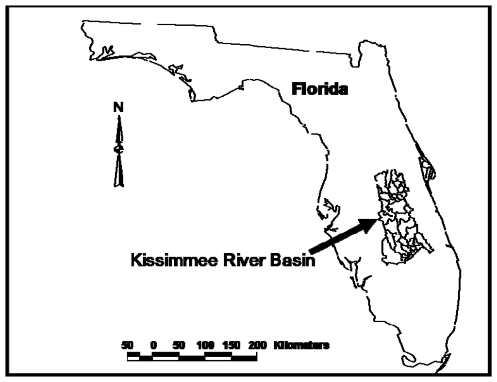
Figure 1.
Location of Kissimmee River basin on the map of Florida.
2.2. Data Sets
2.2.1 Groundwater Data
In order to analyze the effect of restoration on the groundwater levels, monthly water level was analyzed from eight selected monitoring wells from 2000-2004. Wells were selected to represent the different parts of the basin. The location of the selected monitoring wells in this study is shown in Figure 2.
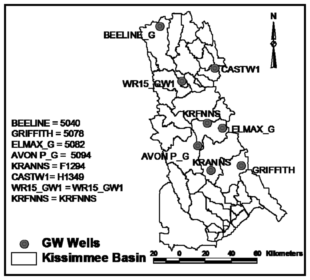
Figure 2.
Location of groundwater monitoring wells.
2.2.2. Remotely-sensed Data
The study considered at assessing the spatiotemporal changes of vegetation cover and latent heat flux (evapotranspiration in energy units) of the basin. Remotely-sensed images from the Moderate Resolution Imaging Spectroradiometer (MODIS) aboard Terra sensor was used in this study. Images for the months of April, September and December from 2000-2004 were acquired and processed. Surface temperature (Ts), normalized difference vegetation index (NDVI) and albedo were also acquired from the Land Processes Distributed Active Archive Center (LP DAAC) ( http://lpdaac.usgs.gov/modis/dataproducts.asp) and used in the surface energy balance computation. Micrometeorological data collected from National Climatic Data Center (NCDC) (NCDC, 2005) include air temperature and wind speed.
2.3. NDVI-TS-Albedo Relationship
From MODIS data, monthly values of NDVI, TS and albedo were generated for the months of April, September and December from 2000-2004. The selection of the months was designed to represent the different times of the year. Using these values as layers, unsupervised classification was run using Iterative Self-organizing Data Analysis (ISODATA) algorithm (ERDAS, 1999). This classification yielded 30 classes for each month. Combining the resulting land-cover classes from each run (3 months x 5 years) gave a scattergram of NDVI- TS -Albedo (Figure 3).
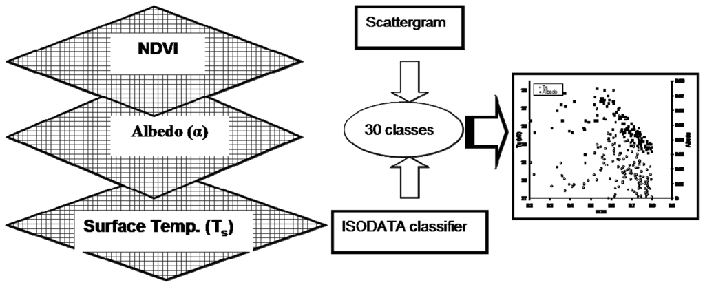
Figure 3.
Flow chart for the scattergram development.
2.4. Fractional Vegetation Cover (FVC) Mapping
The NDVI (Rouse et al., 1974) is a measure of the degree of greenness in the vegetation cover of a watershed. It is the ratio of the difference to the sum of the reflectance values of near-infrared (NIR) and red bands. In highly vegetated areas, the NDVI typically ranges from 0.1 to 0.7, in proportion to the density and greenness of the plant vegetation. Clouds, water and snow, which have larger visible reflectance than NIR reflectance, will yield negative NDVI values. Rock and bare soil areas have similar reflectance in the two bands and result in NDVI values near zero.
To understand the change in the fractional vegetation cover for images of different scenes and dates, the scaled NDVI (NDVIs) has been used by many researchers (Price, 1987; Che and Price, 1992; and Carlson and Arthur, 2000).
Carlson and Ripley (1997) found the relationship between fractional vegetation cover (FVC) and scaled NDVI to be
Where FVC ranges between 0 and 1. The FVC is an indicator of the level of vegetation cover at a pixel level, which is a very good estimate of the percent of pixel area covered by vegetation.
2.5 Latent Heat Mapping
Remote sensing-based evapotranspiration (ET) estimations using the surface energy budget equation are proving to be one of the most recently accepted techniques for areal ET estimation (Morse et al. 2000). Surface Energy Balance Algorithms for Land (SEBAL) is one of such models utilizing Landsat images and images from others sensors with a thermal infrared band to solve equation (3) and hence generate areal maps of ET (Bastiaanssen et al. 1998a; Bastiaanssen et al. 1998b and Morse et al. 2000).
SEBAL requires weather data such as solar radiation, wind speed, precipitation, air temperature, and relative humidity in addition to satellite imagery with visible, near infrared and thermal bands. SEBAL uses the model routine of ERDAS Imagine in order to solve the different components of the energy budget equations.
In the absence of horizontally advective energy, the surface energy budget of land surface satisfying the law of conservation of energy can be expressed as,
where Rn is net radiation at the surface, LE is latent heat or moisture flux (ET in energy units), H is sensible heat flux to the air, and G is soil heat flux. Energy flux models such as SEBAL (Bastiaanssen et al. 1998a; Bastiaanssen et al. 1998b) solve Equation (3) by estimating the different components separately.
With Rn, G, and H known, the latent heat flux is the remaining component of the surface energy balance to be calculated by SEBAL. Rearranging Equation (3) gives the latent heat flux where:
The detailed technique for estimating latent and sensible heat fluxes using remotely-sensed is documented and was tested in Europe, Asia, Africa, and in Idaho in the US and proved to provide good results (Bastiaanssen et al. 1998a; Bastiaanssen et al. 1998b; Wang et al. 1998; Bastiaanssen 2000; Morse et al. 2000, Oberg and Melesse, 2006).
3. Results and Discussion
3.1. NDVI-TS-Albedo Relationship
The scattergram of NDVI-TS-Albedo (Figure 4). shows that, surface temperature and albedo have a negative relationship with the level of green vegetation especially for NDVI >0.5 with R2 value of 0.61 and 0.15, respectively (Figure 4). Higher latent heat losses from the vegetated surface lead to a cooler surface and lower surface temperature in vegetated areas than bare ground. This relationship is not clearly defined in less vegetated surface (water bodies and bare ground) as shown in the left-hand side of the graph (Figure 4). Similarly albedo has also a negative correlation with NDVI for the highly vegetated portion of the basin. For less vegetated surface, this relationship is not distinct (Figure 4).
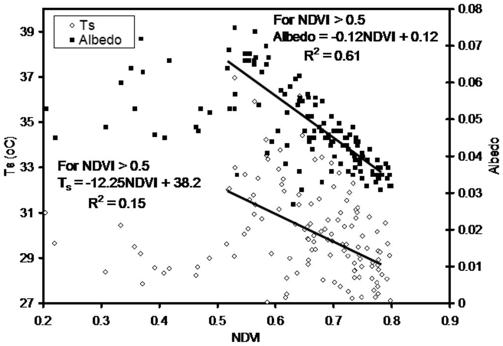
Figure 4.
Scattergram of albedo, NDVI and surface temperature.
3.2. Fractional Vegetation Cover Changes
Fractional vegetation cover (FVC) for the month of April from 2000, 2002 and 2004 was generated and comparisons were made (Figures 5). It is shown that FVC has shown changes along the river, especially in the middle portion of the watershed. Although changes are not significant (mean April FVC of 0.15. 0.16 and 0.17 for 2000, 2002 and 2004, respectively), the trend is an indictor of some response of the vegetation along the river to the restoration work (Table 1). The actual changes in the FVC will require a field sampling and close observation. This study does not identify the type of vegetation and if this response is a desirable one. Table 1 shows statistics of the FVC for the period of the study for the area along the river as shown in Figure 5.
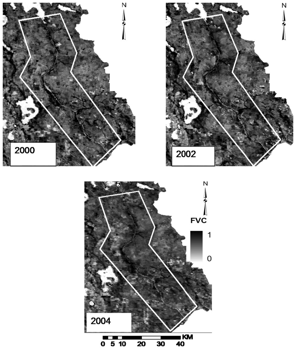
Figure 5.
MODIS-based fractional vegetation cover (FVC) of the area of interest for 2000. 2002 and 2004.

Table 1.
Statistics of average FVC and monthly LE values for the month of April for 2000, 2002 and 2004 for the area of interest along the river.
3.3. Latent Heat Flux Dynamics
Latent heat grids were generated for the month of April (2000, 2002 and 2004). Figures 6 show maps of latent heat in watts per square meter. As it is depicted in Figures 6, latent heat values were higher in 2002 and 2004 than 2000 on areas along the rivers (Table 1). The average April LE for 2000, 2002 and 2004 were 128, 135 and 139 W/m2, respectively. The removal of flood control structures and rechannalization of the river to its natural course will increase the floodplain area and in turn higher latent heat flux. It is shown that higher latent heat flux along the river can be attributed to the increased flood plain areas and vegetation cover. The rainfall depth for the month of April (2000, 2002 and 2004) was 40, 10 and 35 mm, respectively.
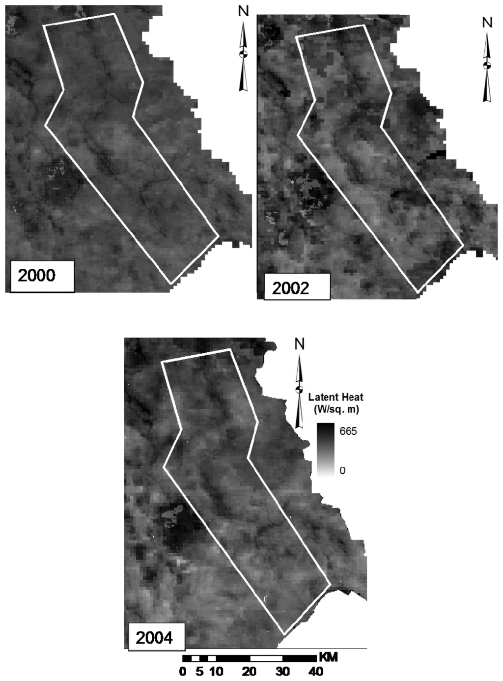
Figure 6.
MODIS-based monthly latent heat flux (W/m2) of the area of interest for 2000. 2002 and 2004.
3.4. Groundwater Data
Groundwater level is an indicator of the response of wetlands to restoration. Change in hydrology of wetlands with shallow groundwater table is used as one of the measure of success of the restoration activity. Eight groundwater monitoring wells were selected to represent the different locations in the basin. Monthly groundwater level from these wells was used and comparisons were made for the period of study. Taking in to account the volume of rainfall for most of the year, it is shown that wells along the rivers has shown a shallower ground water table between 2001 and 2003 (Table 2) compared to the rest of the years (Figure 7). It was also shown that analysis of groundwater level data (2000-2004) from eight monitoring wells showed that, the average monthly level of groundwater was increased by 20 cm and 34 cm between 2000 and 2004, and 2000 and 2003, respectively (Table 2).
Table 2.
Average monthly groundwater levels (m amsl) for selected wells.
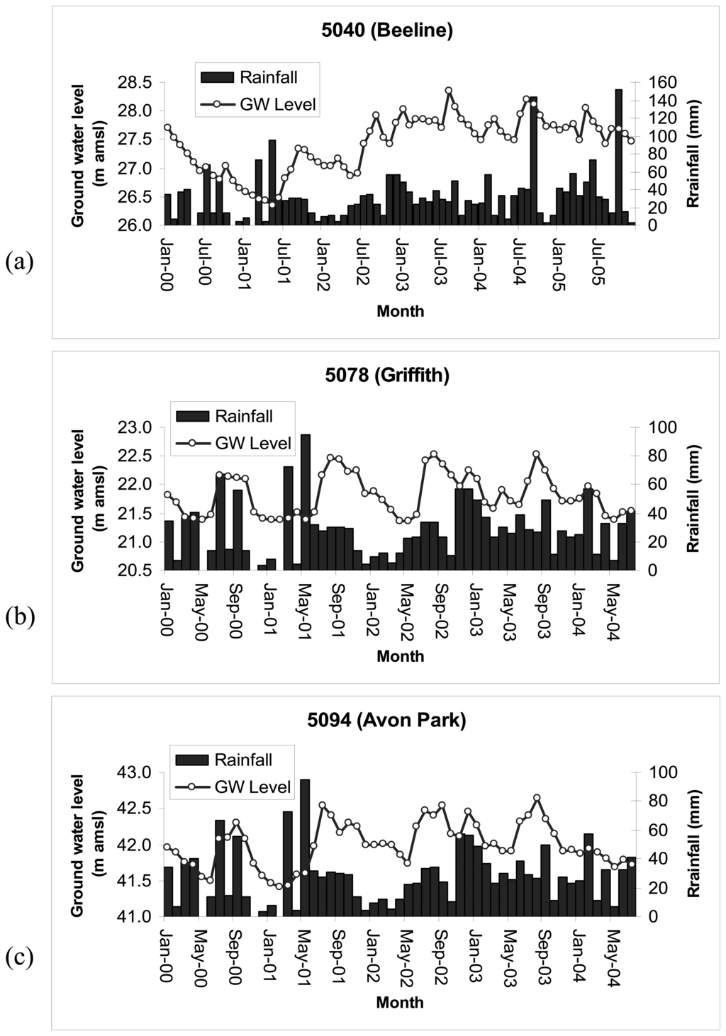

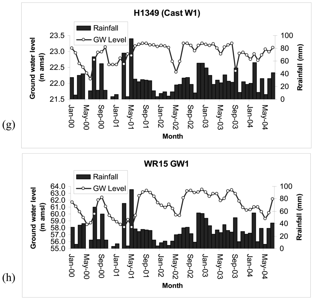
Figure 7.
Monthly groundwater levels of the selected eight monitoring wells and rainfall. (a) 5040 (b) 5078 (c) 5094 (d) 5082 (e) F1294 (f) KRFNNS (g) H1349 (h) R15_GW1
4. Concussions and Summary
Response of the Kissimmee basin's hydrology and vegetation to the recent restoration was evaluated using MODIS-based FVC, spatial latent heat flux and groundwater records. The NDVI-TS-albedo relationship was also analyzed for the 2000-2004 period. Using NDVI, TS and albedo values for the month of April, unsupervised classification was conducted and scattergram was generated. Results show that for the highly vegetated portion of the graph, a negative correlation between NVDI-TS and NDVI-albedo was observed. It was also indicated that for the less vegetated (lower NDVI) part, the NDVI-TS-albedo relationship was not clearly defined.
The fractional vegetation cover was increased for 2002 and 2004 than 2000 for areas along the Kissimmee River indicating response to the floodplain restoration. The spatial latent heat flux, which is evapotranspiration in energy units, has also shown an increase in 2002 and 2004 compared to 2000, which can be attributed to large areas of vegetated surface and change in the hydrology of the area. This change was mainly seen along the river where most of the restoration work is going and changes in the hydrology are expected.
The groundwater level records from selected monitoring wells were also used to compare spatiotemporal variations in the groundwater levels. Analysis of groundwater level data (2000-2004) from eight monitoring wells showed that, the average monthly level of groundwater was increased by 20 cm and 34 cm between 2000 and 2004, and 2000 and 2003, respectively. Taking into account the amount of rainfall, this observation is valid and reasonable. Understanding the complete ecohydrological response of the basin due to the restoration work will require collection and analysis of vegetation cover at finer scales than reported in this study.
Acknowledgments
The authors acknowledge the South Florida Water Management District for the GIS and groundwater flow data. We also acknowledge USGS- Land Processes Distributed Active Archive Center (LP DAAC) for the MODIS data and NCDC for the weather data provided.
References
- Baret, F.; Guyot, G.; Begue, A.; Maurel, P.; Podaire, A. Complimentarily of middle-infrared reflectance for monitoring wheat canopies. Remote Sensing of Environment 1988, 26, 213–215. [Google Scholar]
- Bastiaanssen, W.G.M. SEBAL-based sensible and latent heat fluxes in the irrigated ediz Basin, Turkey. Journal of Hydrology 2000, 229, 87–100. [Google Scholar]
- Bastiaanssen, W.G.M.; Menenti, M.; Feddes, R.A.; Holtslag, A. A. M. The Surface Energy Balance Algorithm for Land (SEBAL): Part 1 formulation. Journal of Hydrology 1998a, 212-213, 198–212. [Google Scholar]
- Bastiaanssen, W.G.M.; Pelgrum, H.; Wang, J.; Ma, Y.; Moreno, J.; Roerink, G.J.; van der Wal, T. The Surface Energy Balance Algorithm for Land (SEBAL): Part 2 validation. Journal of Hydrology 1998b, 212-213, 213–229. [Google Scholar]
- Boyd, D.S.; Foody, G.M.; Curran, P.J.; Lucas, R.M.; Honzaks, M. An Assessment of radiance in Landsat TM middle and thermal infrared wave bands for the detection of tropical regeneration. Int. J. of Remote Sensing 1996, 17, 249–261. [Google Scholar]
- Carlson, T.N.; Arthur, S.T. The impact of land use-land cover changes due to urbanization on surface microclimate and hydrology: a Satellite Perspective. Global and Planetary Change 2000, 25, 49–65. [Google Scholar]
- Carlson, T.N.; Ripley, A.J. On the relationship between fractional vegetation cover, leaf area Index and NDVI. Remote Sensing of Environment 1997, 62, 241–252. [Google Scholar]
- Che, N.; Price, J.C. Survey of radiometric calibration results and methods for visible and near-infrared channels of NOAA-7,-9 and −11 AVHRRs. Remote Sensing of Environment 1992, 41, 19–27. [Google Scholar]
- Clewell, A.F.; Lea, R. 1989; Creation and restoration of forested wetland vegetation in the southeastern United States. Kusler, J.A., Kentula, M.E., Eds.; 1989; In Wetland Creation and Restoration: The Status of the Science; Island Press: Washington, DC; pp. 195–232. [Google Scholar]
- Cole, C.A.; Brooks, R.P. A comparison of the hydrologic characteristics of natural and created mainstem floodplain wetlands in Pennsylvania. Ecological Engineering 2000, 14, 221–231. [Google Scholar]
- Curran, P.J.; Dungan, J.L.; Gholz, H.L. Seasonal LAI in slash pine estimated with Landsat TM. Remote Sensing of Environment 1992, 39, 3–13. [Google Scholar]
- Danson, F.M.; Curran, P.J. Factors affecting the remotely sensed response of coniferous forest plantations. Remote Sensing of Environment 1993, 43, 55–65. [Google Scholar]
- Earth Resources Data Analysis System (ERDAS). 1999; ERDAS Field guide; ERDAS Inc: Atlanta, GA. [Google Scholar]
- French, A.N.; Schmugge, T.J.; Kustas, W.P. Estimating surface fluxes over the SGP site with remotely sensed data. Phys. Chem. Earth 2000, 25(2), 167–172. [Google Scholar]
- Gurnell, A.M.; Hupp, C.R.; Gregory, S.V. Linking hydrology and ecology. Hydrological Processes 2000, 14, 2813–2815. [Google Scholar]
- Hemakumara, H. M.; Chandrapala, L.; Moene, A. F. Evapotranspiration fluxes over mixed vegetation areas measured from large aperture scintillometer. Agricultural Water Management 2003, 58(2), 109–122. [Google Scholar]
- Janssen, R.; Goosen, H.; Verhoeren, M.L.; Verhoeren, J.T.A.; Omtzigt, A.Q.A.; Maltby, E. Decision support for integrated wetland management. Environmental Modeling & Software 2004. [Google Scholar] [CrossRef]
- Kustas, W.P. Estimates of evapotranspiration with a one- and two-layer model of heat transfer over partial canopy cover. J. Appl. Meteorology 1990, 29, 704–715. [Google Scholar]
- Kustas, W.P.; Norman, J. Evaluation of soil and vegetation heat flux predictions using simple two-source model with radiometric temperatures for partial canopy cover, Agric. Forest Meteorology 1999, 94, 13–29. [Google Scholar]
- Kustas, W.P.; Norman, J.M.; Anderson, M.C.; French, A.N. Estimating sub-pixel surface temperatures and energy fluxes from the vegetation index–radiometric temperature relationship. Remote Sensing of Environment 2003, 85(4), 429–440. [Google Scholar]
- Kustas, W.P.; Li, F.; Jackson, T.J.; Prueger, J.H.; MacPherson, J.I.; Wolde, M. Effects of remote sensing pixel resolution on modeled energy flux variability of croplands in Iowa. Remote Sensing of Environment 2004, 92(4), 535–547. [Google Scholar]
- Kustas, W.P.; Perry, E.M.; Doraiswamy, P.C.; Moran, M.S. Using satellite remote sensing to extrapolate evapotranspiration estimates in time and space over a semiarid Rangeland basin. Remote Sensing of Environment 1994, 49(3), 275–286. [Google Scholar]
- Lambin, E.F.; Strahler, A.H. Indicators of land cover change - vector analysis in multi-temporal space at coarse spatial scale. Int. J. of Remote Sensing 1994, 15, 2099–2119. [Google Scholar]
- Land Processes Distributed Active Archive Center (LP DAAC). http://lpdaac.usgs.gov/modis/dataproducts.asp accessed on January 24, 2005.
- Loiselle, S.; Bracchini, L.; Bonechi, C.; Rossi, C. Modeling energy fluxes in remote wetland ecosystems with the help of remote sensing. Ecological Modeling 2001, 45(2), 243–261. [Google Scholar]
- Melesse, A.M.; Jordan, J.D. A Comparison of fuzzy vs. augmented-ISODATA classification algorithm for cloud and cloud-shadow discrimination in Landsat imagery. Photogrammetric Engineering and Remote Sensing 2002, 68(9), 905–911. [Google Scholar]
- Melesse, A.M.; Oberg, J.; Beeri, O.; Nangia, V.; Baumgartner, D. Spatiotemporal Dynamic of Evapotranspiration and Vegetation at the Glacial Ridge Prairie Restoration. Hydrological Processes 2006, 20(7), 1451–1464. [Google Scholar]
- Melesse, A.M.; Nangia, V. Spatially distributed surface energy flux estimation using remotely-sensed data from agricultural fields. Hydrological Processes 2005, 19(14), 2653–2670. [Google Scholar]
- Mitsch, W.J.; Gosselink, J.G. 2000; Wetlands; John Wiley & Sons: New York. [Google Scholar]
- Mohamed, Y.A.; Bastiaanssen, W.G.M.; Savenije, H.H.G. Spatial variability of evaporation and moisture storage in the swamps of the upper Nile studied by remote sensing techniques. Journal of Hydrology 2004, 289, 145–164. [Google Scholar]
- Morse, A.; Tasumi, M.; Allen, R.G.; Kramber, W. 2000; Application of the SEBAL methodology for estimating consumptive use of water and streamflow depletion in the Bear River basin of Idaho through remote sensing. Final report submitted to the Raytheon Systems Company; In Earth Observation System Data and Information system Project; by Idaho Department of Water Resources and University of Idaho; p. 107pp. [Google Scholar]
- Myers, R.S.; Shaffer, G.P.; Llewellyn, D.W. Bald Cypress restoration in Southeast Louisiana: the relative effects of herbivory, flooding, competition, and macronutrients. Wetlands 1995, 15(2), 141–148. [Google Scholar]
- National Climatic Data Center (NCDC). 2005. http://climvis.ncdc.noaa.gov/cgi-bin/ginterface accessed on June 13, 2005.
- National Research Council. 1995; Wetlands Characteristics and Boundaries.; National Academy Press: Washington, DC. [Google Scholar]
- Niswander, S.F.; Mitsch, W.J. Functional analysis of a two-year-old created in-stream wetland: hydrology, phosphorus retention, and vegetation survival and growth. Wetlands 1995, 15(3), 212–225. [Google Scholar]
- Panigrahy, S.; Parohar, J.S. Role of middle-infrared bands of Landsat Thematic Mapper in determining the classification accuracy of rice. Int. J. of Remote Sensing 1992, 13, 2943–2949. [Google Scholar]
- Price, J.C. Calibration of satellite Radiometers and the comparison of vegetation indices. Remote Sensing of Environment 1987, 21, 15–27. [Google Scholar]
- Price, J.S.; Waddington, J.M. Advances in Canadian wetland hydrology and biogeochemistry. Hydrological Processes 2000, 14, 1579–1589. [Google Scholar]
- Oberg, J.; Melesse, A.M. Wetland Evapotranspiration Dynamics vs. Ecohydrological Restoration: An Energy Balance and Remote Sensing Approach. J. of American Water Resources Association 2006, 42(3), 565–582. [Google Scholar]
- Quinn, N.W.T.; Hanna, W.M. A decision support system for adaptive real-time management of seasonal wetlands in California. Environmental Modeling & Software 2003, 18, 503–511. [Google Scholar]
- Raghunathan, R.; Slawecki, T.; Chen, Z.Q.; Dilks, D.W.; Bierman, V.J.; Wade, S. Exploring the dynamics and fate of total phosphorus in the Florida Everglades using a calibrated mass balance model. Ecological Modeling 2001, 142, 247–259. [Google Scholar]
- Rouse, J.W.; Haas, R.H.; Schell, J.A.; Deering, D.W. Monitoring vegetation systems in the Great Plains with ERTS. Proc. Third Earth Resources Technology Satellite-1 Symposium, Greenbelt: NASA SP 1974, 351, 3010–3017. [Google Scholar]
- Williams, G.E.; Anderson, D.; H Bousquin, S. G.; Carlson, C.; Colangeleo, D.J.; Glenn, J.L.; Jones, B.L.; Koebel, J.W.; Jorge, J. 2007; Chapter11: Kissimmee River Restoration and Upper Basin Initiation; Redfield, G., Ed.; The 2007 South Florida Environmental report; South Florida Water Management District: West Palm Beach Florida. [Google Scholar]
- Spanner, M.A.; Pierce, L.L.; Running, S.W.; Peterson, D.L. The seasonality of AVHRR data of temperate coniferous forests: Relationship with LAI. Remote Sensing of Environment 1990, 33, 97–112. [Google Scholar]
- Stone, T.A.; Schleeinger, P.; Houghton, R.A.; Woodwell, G.M. A map of the vegetation of South America based on satellite imagery. Photogrammetric Engineering and Remote Sensing 1994, 60, 541–551. [Google Scholar]
- Stover, D. Engineering the Everglades. Popular Science 1992. [Google Scholar]
- Toth, L.A. 1996; Restoring the hydrogeomorphology of the channelized Kissimmee River. pp. 369–383. Brookes, A., Shields, F.D., Jr., Eds.; In River channel restoration: guiding principles for sustainable projects.; John Wiley & Sons, Ltd.: Chichester, England. [Google Scholar]
- Tucker, C.J.; Dregne, H.E.; Newcomb, W.W. Expansion and contraction of the Sahara desert from 1980 to 1990. Science 1991, 253, 299–302. [Google Scholar]
- Wang, J.; Bastiaanssen, W.G.M.; Ma, Y.; Pelgrum, H. Aggregation of land surface parameters in the oasis-desert systems of Northwest China. Hydrological Processes 1998, 12, 2133–2147. [Google Scholar]
- Wilson, R.F.; Mitsch, W.J. Functional assessment of five wetlands constructed to mitigate wetland loss in Ohio. Wetlands 1996, 16(4), 436–451. [Google Scholar]
© 2007 by MDPI ( http://www.mdpi.org). Reproduction is permitted for noncommercial purposes.