1. Introduction
There is growing interest in hyperspectral remote sensing for research and applications in a variety of fields, including geology, agriculture, forestry, coastal and inland water studies, environmental hazards assessment, and urban studies [
1,
2]. The concept of hyperspectral imaging originated from geological applications in the early 1980s, mainly for the purpose of mineral exploration [
3]. Imaging spectrometers acquire data in many contiguous narrow bands leading to a complete reflectance or emittance spectrum for each pixel of the wavelength region covered.
Until recently imaging spectroscopy was an expensive tool due to the limitations to airborne systems. Existing airborne hyperspectral sensors such as AVIRIS (Airborne Visible / InfraRed Imaging Spectrometer), casi (compact airborne spectral imager) or HYMAP (HYperspectral MAPping) are one-of-a-kind sensors supported by large, dedicated programs. They have proven useful for many applications, but are difficult to schedule due to many competing user requirements. Therefore airborne imaging spectrometer systems are cost-intensive for the user and the availability for multi-temporal applications is low. A high temporal resolution is required for environmental analysis because most developments either in natural or in managed ecosystems can only be monitored through time series of remote sensing observations. In 1997 these drawbacks led to the idea of a compact light-weight imaging spectrometer to overcome the difficulties of the existing systems and provide data for the environmental research purposes of the Department for Geography of the Ludwig-Maximilians-University in Munich (Germany). This was the birth of the AVIS (Airborne Visible / Infrared imaging Spectrometer) system.
The ongoing development of digital imaging tools enabled the enhancement of the first generation of AVIS to AVIS-2. Dedicated software was developed to acquire and process the data. Since 2001 AVIS-2 is being operated and will form the basis of this paper.
2. System Specifications
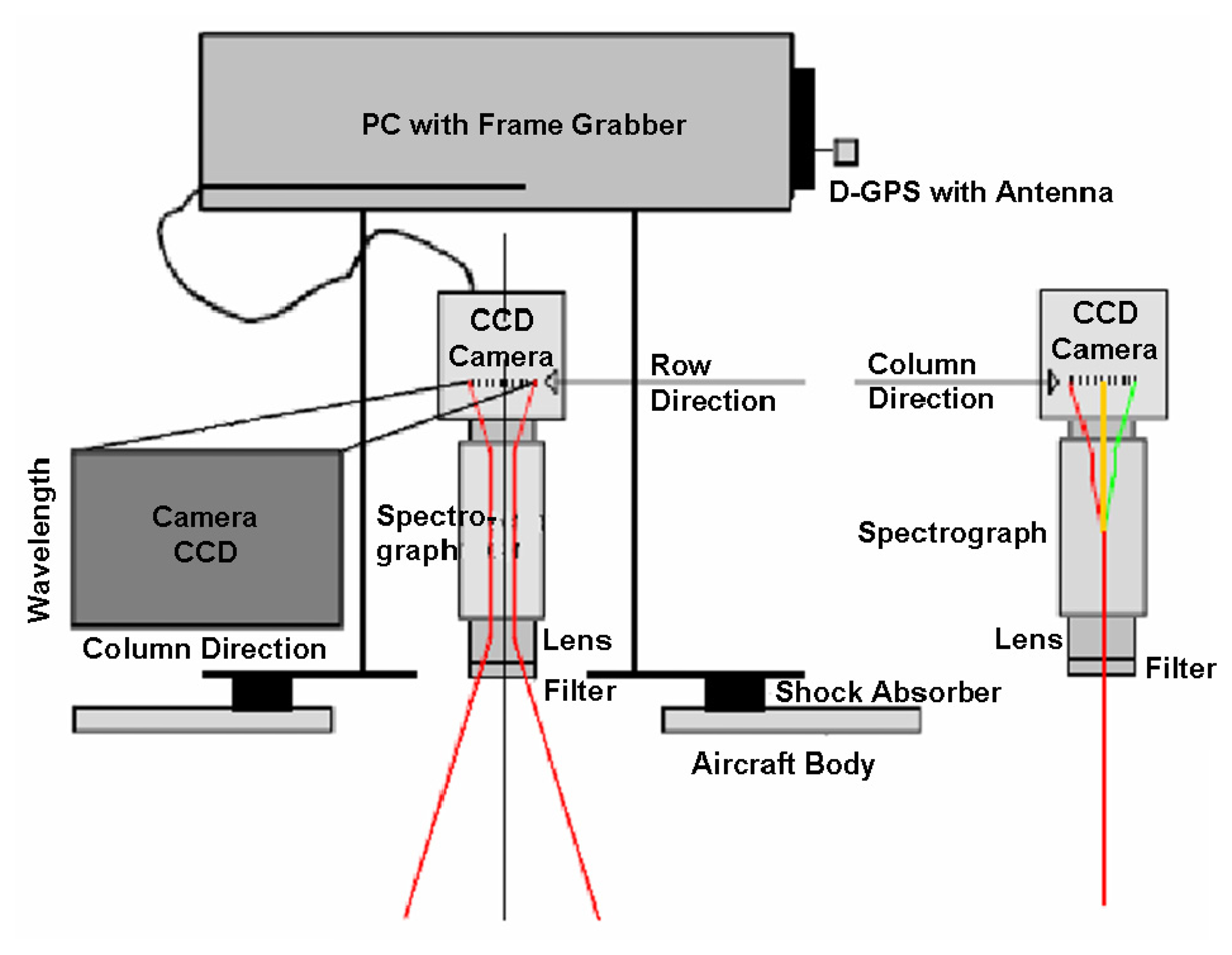
The specifications of the AVIS system were determined by the availability and affordability of components resulting in a Charged Coupled Device (CCD)-based system operating in the visible (VIS) to near infrared (NIR) spectral domain. AVIS is conceived to be operated on different platforms such as Dornier DO-27, DO-228 and microlight aircrafts, where the sensor is mounted on vibration dampening mounts.
The components of the system are shown in
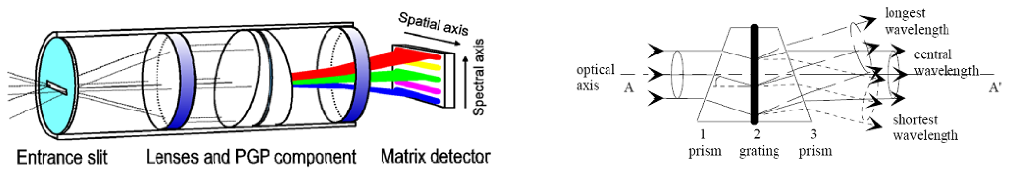
Figure 1. AVIS-2 is based on a spectrograph (IMSPECTOR, Specim Inc.), which is mounted onto a black and white 2/3″ CCD-video camera (VOSSKüHLER 1300QLN) and a filter-lens system (f/1.4, 8 mm; SCHNEIDER Optics;. Radiation which enters the spectrograph slit is collimated by the first lens and refracted at the prism surface to the correct incident angle of the holographic grating (
Figure 2). The grating disperses the light according to the common grating
Equation 1 [
5].
where
| s | grating spacing [nm], |
| θm | angle between the direction of wave travel and direction of m-order [°], |
| m | order of spectrum, and |
| λ | wavelength [nm]. |
Any tubular optics are sensitive to ghost images and scattered light caused by reflections at optical surfaces. There is also a risk of light scattering caused by transmitted, unwanted orders of diffraction in the holographic grating. These are taken into account by using baffles inside the tube as well as multilayer coatings of all air/glass surfaces. The tilted surfaces of the prisms refract remaining forwarded reflections to blackened surfaces of the spectrometer tube leading to a distortion due to scattered light of less than 1 % [
5,
6].
Spatial information at the entrance slit is transferred to the imaging plane along the axis parallel to the slit length direction (spatial axis in
Figure 2). The output of the spectrograph is a column of 512 pixels (spectral axis in
Figure 2) representing the wavelengths from 400 to 900 nm with a spectral sampling rate of 3.7 nm. The spatial output of the spectrograph is a row of 640 pixels.
The spectrograph is mounted onto a 2/3″ CCD-camera (VOSSKüHLER 1300QLN). The primary selection criteria for the camera were a progressive interline-transfer sensor and asynchronous operation mode (image on demand) which enables very short exposure times up to 1/10000 s with full resolution (1280 × 1024 pixel;. This enables the monitoring of moving targets or the monitoring of fixed targets with the camera being moved. When the system is moved above ground, a two-dimensional flight line is created. The high resolution output of the camera is binned to a 640 × 512 image to increase the signal-to-noise ratio. Data rates are typically less than 15 MB/s, but several gigabytes may be stored during a flight line. The data is viewed in real-time on the monitor to check data quality.
A Microsoft Windows NT-based personal computer (PC) controls the camera through a PCI interface card. Software was developed to configure the camera for the particular mode desired, including gain, frame rate, and number of frames to collect. The signal is digitized via a frame grabber and stored in a standard file format on a hard disk of the connected PC together with additional data from a differential Global Positioning System (dGPS, GARMIN) and an Inertia Navigation System (INS, iMAR GmbH), which are mounted on the same plate as the camera. The dGPS/INS data are stored in the header of each image line and allow a line-by-line positioning during the geometric correction of the images (section 3.3.3).
3. Calibration and Processing
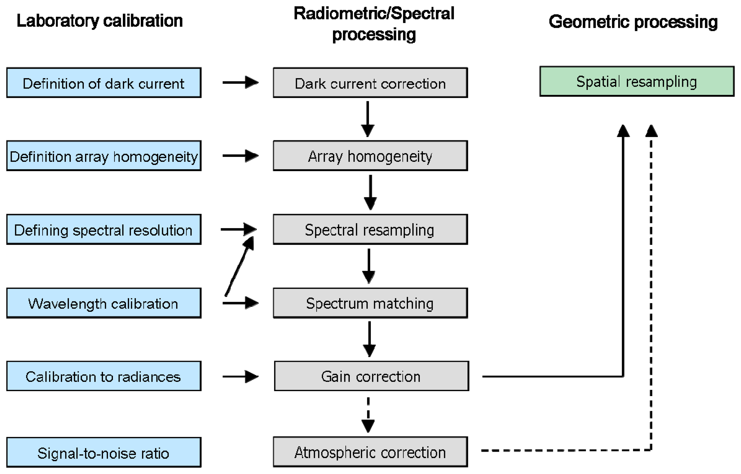
Pushbroom type imaging spectrometers offer advantages in robustness, integration time, speed, and spectral/spatial resolution. Nevertheless, they also suffer from some intrinsic sources of malfunction or defects, which have to be addressed by appropriate correction schemes. Malfunctions inherent to the system or temporally consistent sensor defects can be analyzed in the laboratory. Correction schemes can therefore be implemented in the radiometric or spectral processing of the data. This has to be carried out each time the system composition or system settings are changed. The calibration and processing chains necessary for an appropriate evaluation of the AVIS-2 data are presented in
Figure 3 and will be described in more detail in the following sections.
3.1 Radiometric properties and calibration
The analysis of a sensor's radiometry provides information essential for the handling of imaging spectrometer data. The radiometric resolution is one of the most dominant features of radiometric properties because it defines the number of grey values into which the incoming radiance can be resolved. The radiance measured by a system is influenced by factors such as changes in scene illumination, atmospheric conditions, viewing geometry, and instrument characteristics. The temporally consistent characteristics of AVIS-2 are analyzed and corrected during the processing of the data. These characteristics are described in this paper including the analysis of dark current, homogeneity of the CCD, and the signal-to-noise ratio.
3.1.1 Radiometric resolution
The radiometric resolution of a system is limited by the lowest radiometric resolution of its components. The camera offers 12 bit imaging on an array of 1280 x 1024 pixels and a 14 bit imaging on 640 x 512 pixels via two by two binning. By using the 640 x 512 pixel mode and additional software binning by a factor of four in the spectral direction, an effective radiometric resolution of 15 bits can be achieved. The nominal spatial resolutions of the acquired images are reduced to 640 pixels in the spatial direction and 128 pixels in the spectral dimension. Besides the increase of bit depth the advantage of binning is the reduction of noise. Furthermore binning enables the camera to increase the image rate from 12.5 frames/s to 25 frames/s.
3.1.2 Dark current
Dark current is caused by thermally generated electrons within the camera. The dark current density can be analyzed by measuring the spectral response for a given temperature with closed aperture. For AVIS-2 the dark current is a constant offset (binned DN = 1180), which is subtracted pixel by pixel from the original data during pre-processing (
Equation 2).
where
| DNdcc | dark current corrected grey value [digital number], |
| DNorg | original grey value [digital number], and |
| DNdark | dark current [digital number]. |
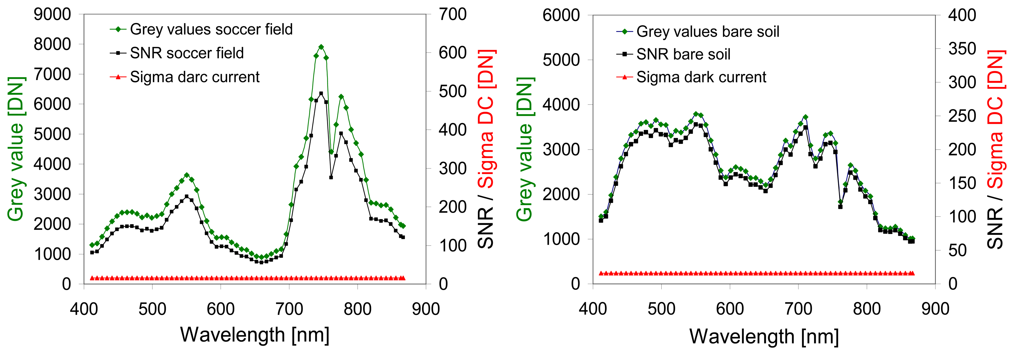
3.1.4 Signal-to-noise ratio (SNR)
Once the data is corrected for dark current and array homogeneity, the SNR analysis can be carried out. This is done in the laboratory using the same illumination equipment as described above. The SNR of the AVIS-2 system at full illumination, as defined in
Equation 3, can be rated at a maximum of 66 dB (2000 : 1) for the unbinned data.
where
| DNsat | grey value just before saturation [digital number], and |
| σdark | standard deviation of the dark current image. |
The SNR in the image data depends on the illumination conditions, the exposure time and the targets monitored. Examples of a vegetated surface (soccer field) and bare soil are presented in
Figure 5.
3.2 Spectral properties and calibration
In the discussion of spectral properties of imaging spectrometers the spectral resolution, spectral sampling interval and centre wavelengths are the most important parameters. Assuming a Gaussian shaped response function, the spectral resolution is defined as the full width half maximum (FWHM) of the function. The center wavelength is the peak response of the spectrometer to an infinitesimally narrow emission line [
7,
8]. The spectral sampling interval is the distance between two adjacent center wavelengths. Other effects which have to be considered are the analysis of spectral uniformity and responsivity.
3.2.2 Spectral Resolution
The nominal spectral resolution of the spectrograph is 7 nm [
5]. To check this specification the real spectral resolution was measured by correlating measured and modeled at-sensor radiances of the oxygen absorption around 760 nm. The oxygen absorption is a suitable feature because of its characteristic shape with two adjacent absorption peaks (
Figure 7).
Therefore, at-sensor radiances were simulated for skylight using MODTRAN 4.2 [
6,
7] with different spectral resolutions (0.5 to 10 nm in steps of 0.5 nm). These simulated radiances were compared with AVIS-2 measurements of skylight resulting in a best fit for a spectral resolution of 9 nm. Therefore the real spectral resolution can be defined as 9 nm. Knowing the band number of the oxygen absorption and the spectral resampling rate the actual wavelength range of AVIS-2 can be identified as covering the spectral region from 404 nm to 875 nm.
3.2.3 Spectral sampling and resampling
AVIS-2 covers the wavelength region between 404 and 875 nm with a sampling interval of 3.7 nm. With an actual spectral resolution of 9 nm, the system is oversampled by the factor 2.4.
Therefore the data were resampled to a spectral sampling rate corresponding closely to the spectral resolution. The averaging was done assuming a Gaussian-shaped response function represented by the different weights for the adjacent bands:
where
By incrementing i a total of 64 resampled spectral bands with a nominal bandwidth of 7.3 nm is produced from the original 128 AVIS-2 bands. This enables the reduction of the amount of data as well as an increase of the SNR without any loss of spectral information.
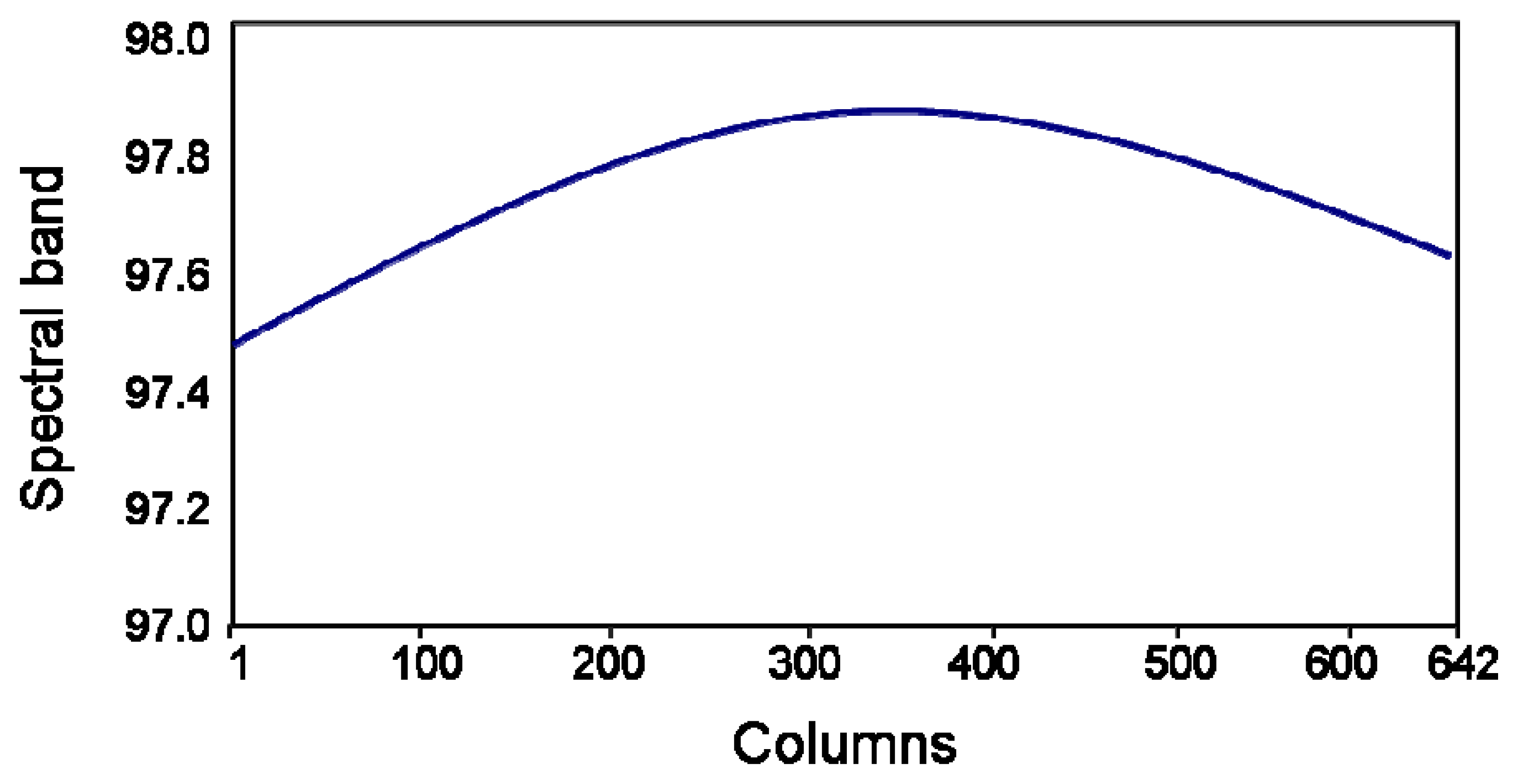
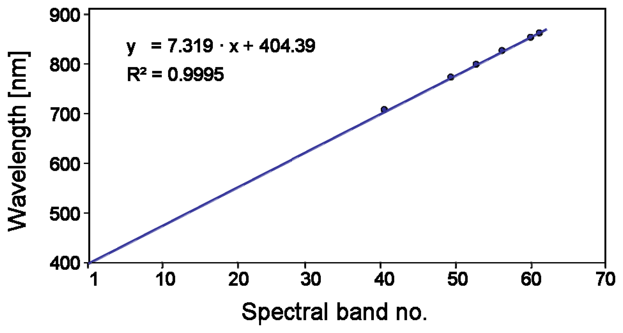
3.2.4 Wavelength calibration
An accurate wavelength calibration is essential for the retrieval of land or ocean surface reflectances. Especially as the atmospheric gas absorption features are very sharp, errors in wavelength calibration can produce significant errors in the resulting reflectances around these features. A wavelength calibration of the spectrograph had already been carried out by the manufacturer. The center wavelengths changed during resampling, therefore the newly defined wavelengths must be checked. This is done using atomic emission lines from a discharge lamp because most atomic emission lines are known with an accuracy exceeding the requirements of calibration [
9,
12]. The measurements were performed in the darkened laboratory using a krypton lamp as the illumination source. Before analysis the correction for dark current and spatial uniformity was performed as well as the resampling to 64 spectral bands. The results presented in
Figure 8 confirm that resampling procedure does not affect the correct wavelength assignment. The deviations turned out to be smaller than the original sampling interval of 3.8 nm.
According to the resampling and wavelength assignment it can be concluded that AVIS-2 operates in the wavelength region between 404 nm and 875 nm with a spectral resolution of 9 nm and a spectral sampling interval of 7.3 nm.
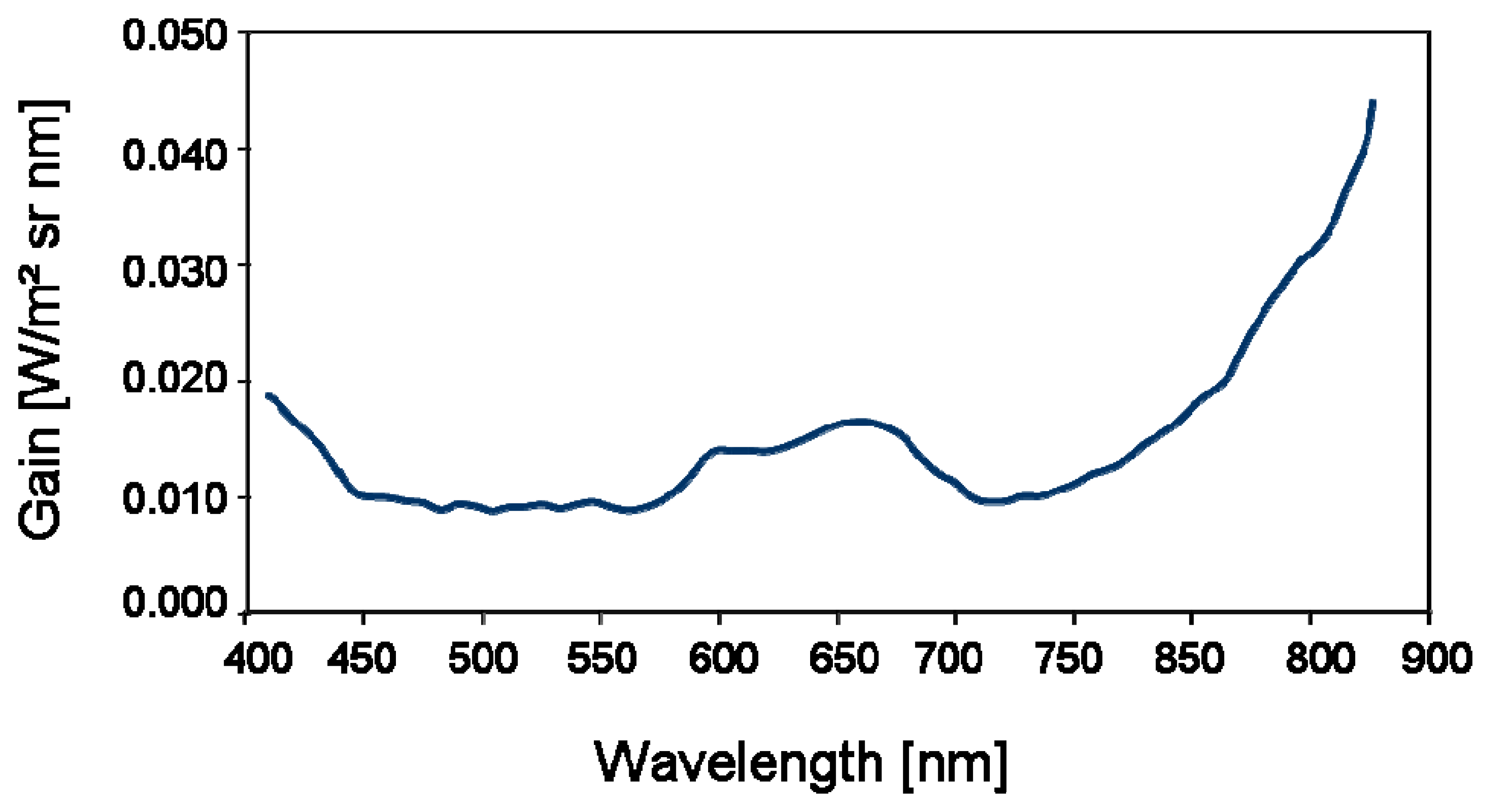
3.2.5 Spectral responsivity
The spectral responsivity of AVIS-2 is the result of the responsivities of its components (spectrograph, camera, lens and filter). The spectral responsivity can be analyzed in the laboratory using an integrating sphere and a halogen calibration lamp (OCEAN OPTICS HL-2000) as the illumination source. The intensity of the output from the sphere is determined by performing a transfer calibration from the calibration lamb. The resulting overall efficiency of light collection by the system is highest between 470 and 570 nm and around 720 nm, which results in a calibration gain that is higher at the wavelengths in the blue, red and towards the NIR (
Figure 9).
The data are used to calculate a relationship between grey values and at-sensor radiances for each spectral band according to
Equation 5.
where
| SRi | spectral at-sensor radiance for band i [W/m2 sr nm], |
| DNi | grey value for band i [DN], |
| DNdark,i | dark current offset for band i [DN], and |
| gi | spectral sensitivity calibration gain [W/m2 sr nm]. |
3.3 Geometric properties and correction
The main parameters of interest concerning the geometry are the spatial resolution of the imagery, the field of view (FOV) and the instantaneous field of view (IFOV). The spatial resolution and the FOV depend strongly on the flight altitude, while the IFOV is constant. The IFOV of a system depends on both the spectrograph and the camera.
Remote sensing data corrections in the spatial domain are well known for image registration and rectification processes [
13,
14]. In satellite remote sensing, the processing normally affects the spatial dimension of the imagery and is usually to be performed within a distance of 0.1 to 2 pixels. Airborne imagery may have more distinct distortions due to dynamic platform movements caused by turbulence in the lower atmosphere.
A major precondition for successful geometric resampling is that the data is radiometrically corrected and calibrated to physical units (e.g. radiance) [
12,
13].
3.3.1 Spatial resolution and ground sample distance
In general the spatial resolution on ground (R) depends strongly on the altitude of the sensor. The spatial resolution of airborne imagery can differ between an image line (cross track) and the movement of the aircraft (along track). Therefore both resolutions have to be calculated separately. The former is determined by the camera pixel size and the point spread size of the optics, which is 30 μm corresponding to a modular transfer function of 15 line-pairs/mm. With an array dimension of 8.8 mm, the point spread size limited resolution is 8800/30 ≅ 300 points [
5]. The resulting spatial resolution on ground can be calculated according to
Equation 6 using the altitude of the aircraft (
h). The latter is determined by the line width of the system (W = 2.98 mrad) and the altitude (see
Equation 7).
According to
Equation 8 the ground sample distance (
GSD) cross track is always determined by the number of pixels of the camera. The along track sampling depends on the frame rate (
i) and the aircraft speed (
v) (see
Equation 9).
3.3.2 Field of view and instantaneous field of view
The field of view (FOV), normally expressed as the cone angle within which incident radiation is focused on the detector, is determined by the lens. The AVIS-2 system uses an IR compensated (400 – 1000 nm) lens with a FOV of 1.16 rad or 66°.
The instantaneous field of view represents the angle viewed by the CCD for each pixel. Comparable to the spatial resolution of an airborne instrument, it can be distinguished between the IFOV along an image line and the IFOV in the direction of aircraft motion.
The IFOV along an image line (
IFOVcross track) is determined by the FOV of the lens and the number of pixels per image line (
Nc = 640) according to
Equation 10. The resulting
IFOVcross track for AVIS-2 is 1.81 mrad before binning.
The IFOV in direction of the aircraft movement (
IFOValong track) is determined by the width of the spectrograph slit (
Ws = 13 μm) and the focal length of the camera (
f = 8.4 mm). According to
Equation 11 it can be rated at 1.55 mrad.
3.3.3 Geometric correction
A dGPS/INS system provides accurate data for geometric processing of the data. The aircraft location (latitude, longitude and altitude) and pointing information (roll, pitch and yaw) are measured with an accuracy of 1.2 mrad at a frequency of 40 Hz.
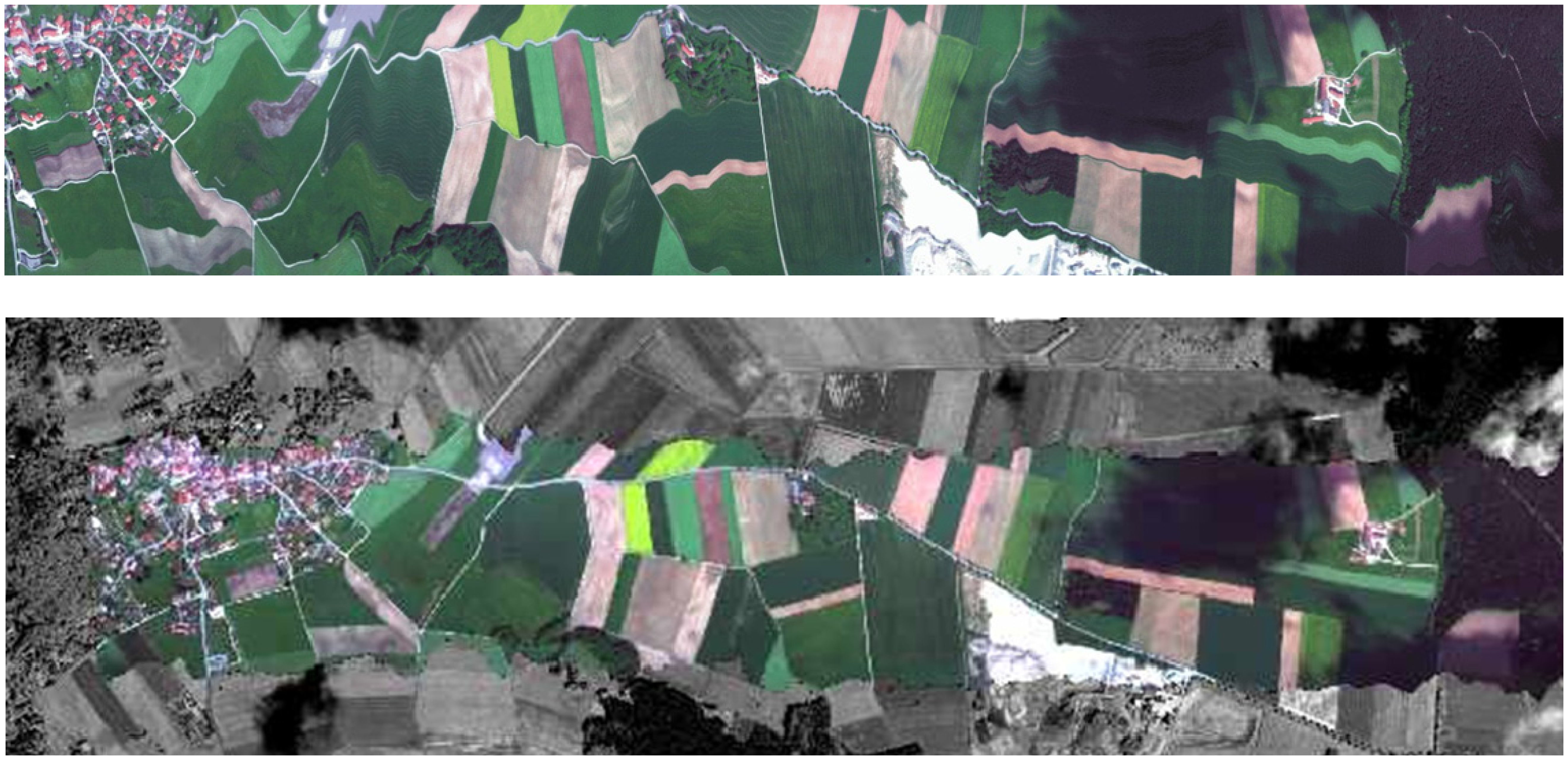
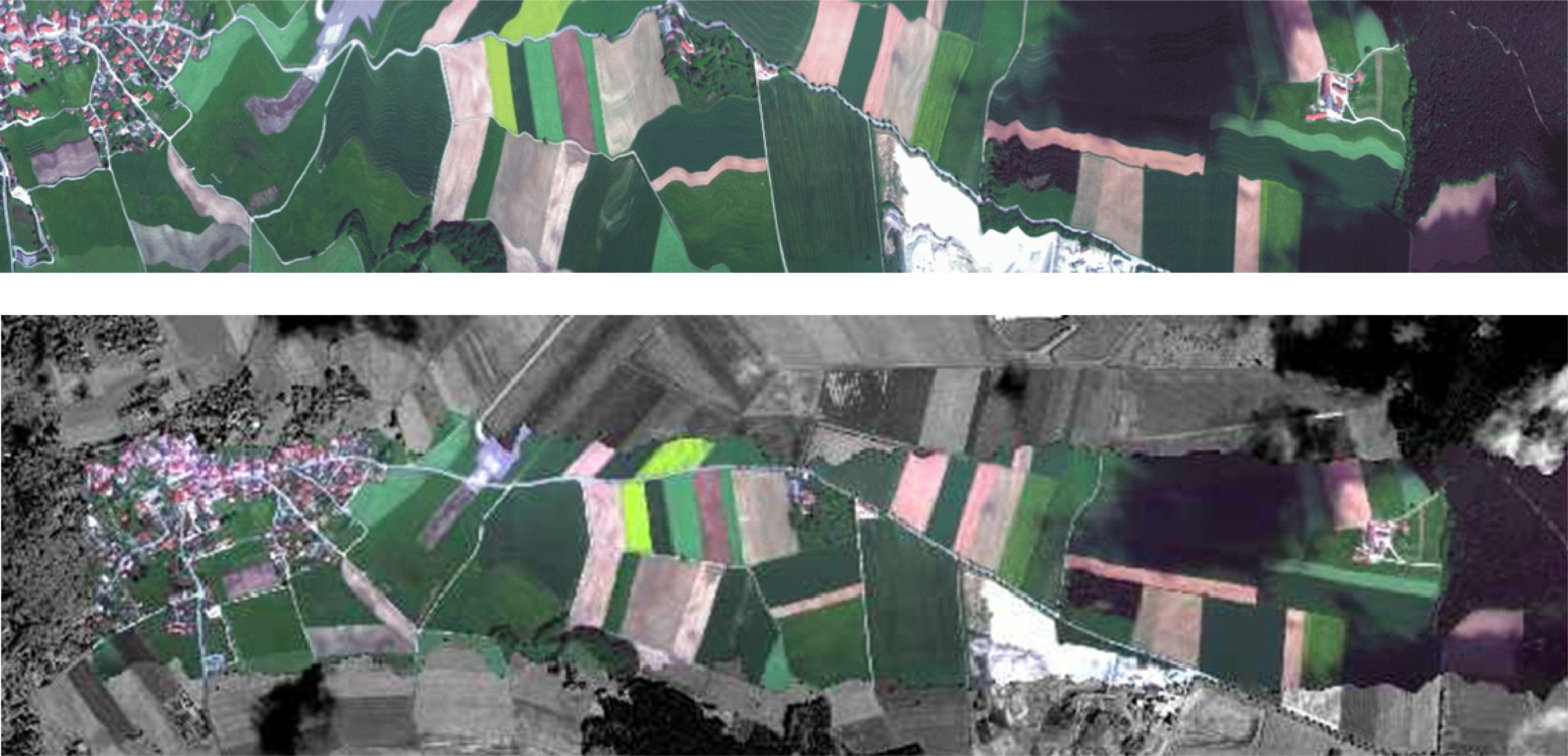
Figure 11 demonstrates the results of the geometric processing of original flight data using INS/GPS data. The INS/GPS data together with a digital terrain model makes it possible to compensate for the motion of the aircraft and at the same time produces an image that closely matches WGS-84 UTM projection. The image was acquired at a flight altitude of 1450 m above ground with a ground speed of 25 m/s and a frame rate of 12 images/s.
4. Examples for the application of AVIS-2 data
The sensor AVIS-2 was/is used for various applications in agriculture [
4,
15,
16,
17,
18], floristic studies [
19,
20,
21], inland water applications [
22] as well as for studies funded by the European Space Agency [
23,
24,
25]. Some examples for AVIS-2 applications will be given in the following section.
4.1 Derivation of reflectance spectra
Figure 13 shows a flight line acquired with AVIS-2 mounted on a microlight plane, which can be observed in
Figure 12.
The data were gathered near the city of Leipzig, Germany, in 2005 within the scope of a project funded by the Centre for Environmental Research Leipzig-Halle (UFZ). The data were gathered at an altitude of 730 m above ground leading to a GSD
cross track of 2.4 m (
Equation 8) and 2.2 m along track (
Equation 9). The data were resampled to a spatial resolution of 2 m. The swath width (
SW) can be calculated at 948 m using
Equation 12.
where
| FOV | 66°, and |
| h | altitude above ground [m]. |
The area monitored in
Figure 13 is located West of the city of Leipzig in a landscape dominated by opencast mining. The natural and man-made reclamation of areas affected by mine-related activities is one research theme of interest in this part of Germany. Opencast mining often gives rise to lakes. In the future these lakes will make up 25% to 30% of all standing water bodies in Germany [
26]. Several mining lakes can be seen on the left part of the image surrounded by an agricultural area and small settlements which are visible on the right. The data are geometrically and radiometrically corrected. Atmospheric correction and reflectance calibration were conducted using software based on MODTRAN 4.2 [
6,
7].
Reflectance spectra of single pixels are presented in
Figure 14. The selected land cover types range from surfaces such as bare soil, meadow or wooded areas to mining lakes, a soccer field or impervious areas. The spectra cover the spectral range from 411 – 875 nm and show characteristic spectral features of vegetation such as the chlorophyll absorption features in the red and the blue as well as the steep increase (red edge) towards the NIR and the NIR-plateau. Different depths of water bodies can clearly be distinguished in the VIS. The shallower the water body the more contribution of the substrate at the bottom of the lakes can be observed and the higher the reflectances are in the blue and green wavelengths [
27].
4.2 Assessment of soil degradation in semi-arid areas
In November 2005, AVIS-2 was operated within the scope of an airborne campaign funded by the European Space Agency (ESA), which was carried out in Southern Tunisia. The objective of the AquiferEx project was to build up a data base of multi-frequency radar (E-SAR) data as well as hyperspectral data suitable for the development and validation of science products to be developed by the project team of ESA's Aquifer [
28], in particular by the companies VISTA (
www.vista-geo.de) and GAF (
www.gaf.de). The campaign was initiated within the scope of the TIGER (Use of Space Technology for Integrated Water Resources Management in Africa) initiative of ESA and UNESCO (United Nations Educational, Scientific and Cultural Organization) with the aim of assisting African countries to overcome problems with an integrated water resource management. Aquifer and AquiferEx had the aim in providing research and development products demonstrating the future capabilities of Earth Observation to support water management [
25,
28,
29].
For the AquiferEx campaign, two test sites were selected in the Tunisian Djeffara (
Figure 15), which is a sub-aquifer of the SASS (Systeme d'Aquifer du Sahara Septentrional), a transboundary ground water body extending over Algeria, Libya, and Tunisia. During the campaign, AVIS-2 was operated in parallel with the Experimental airborne Synthetic Aperture Radar system (E-SAR) by the German Aerospace Center (DLR). Both sensors were mounted on a Do-228 aircraft owned and operated by DLR. The flights were accompanied by ground measurements which were carried out contemporaneously.
The test site Ben Gardane which is shown in
Figure 15 is representative for the southern part of the Tunisian Djefarra and includes mainly pasture and olive plantations. About 26 % of the area is grown with cereals, vegetables and forage crops, where irrigation is performed. Each year about 2.7 Mio m
3 of water is exploited and partly used for irrigation [
23].
The major problem in this region is the intrusion of sea water into the ground water body. During the last decades the pressure within the aquifer has reduced due to massive extraction of ground water for industrial and agricultural purposes leading to an invasion of salty sea water into the ground water. At the present time, the average content of salt in the ground water is 5 - 6 g/l [
23]. The salinity of the ground water and therefore of the soil, the aeolian erosion and low precipitation (< 120 mm/a) lead to land degradation [
23]. Until today, the percentage affected by degradation can only be assumed. About 70 % (without the Sahara desert) of Tunisia is estimated to be affected by different levels of degradation [
29]. The development of a refined land use and land cover mapping using both radar and hyperspectral data were a first attempt to cope with this problem [
28].
Figure 16 presents a land use classification on the basis of AVIS-2 and E-SAR data, demonstrating the high percentage of saline soil in this area.
5. Conclusions
AVIS-2 was designed to produce high quality hyperspectral imagery for environmental monitoring purposes. The sensor was designed as an affordable tool to overcome the competing user requirements of existing airborne systems such as HYMAP, casi or AVIRIS. Therefore all components are commercially available.
The radiometric, spectral and geometric calibration and processing chains have been presented as well as exemplary AVIS-2 reflectance spectra. AVIS-2 turned out to be a valuable sensor for research and applications in a variety of fields such as agriculture, inland water studies and forestry. The specifications of AVIS-2 are summarized in
Table 1.


