Development of Standardization and Management System for the Severity of Unpaved Test Courses

Abstract

The vibration environment essentially accompanied by vehicle operation on the ground is determined by the shape of road surface, which is called as profile. This paper focuses on the development of profile measurement and severity analysis system for unpaved test courses. In general, the profile and severity of unpaved road is an important issue in the reliability of endurance test. In order to measure and maintain unpaved road profile and severity, it is necessary to develop a profilometer system. The developed profilometer system is composed of data processing computer, power unit, air compressor and sensors(encoder, vertical gyro and laser displacement). This study presents the measuring system configuration, measurement principle of road profile and analysis method of road characteristics used at CPG (Chang-won Proving Ground) for this purpose. In order to standardize and manage the severity of unpaved test courses, neural network is applied

1. Introduction

In the development of the vehicles, the Durability test known as life cycle test is essentially performed to evaluate a reliability of vehicles. The test offers important data to determine life cycle of vehicles through the analysis of cost vs. effect, and the test data is used for evaluating and predicting defects of main parts of vehicle during life cycle.

One of the important test factors in endurance test is vibration environments while vehicles are operated. The environment affects the reliability of vehicles owing to fatigue. Therefore, the measurement of road profile and evaluation of profile characteristic are important points to get reliable endurance test results [1-3].

An endeavor, measuring profile and analyzing the severity and then applying the results, has been studied for a long time in the endurance test field. Early, managers of test road have used their experience and subjective measuring method. They have developed the various measuring methods to get more objective results.

In 1970s, the APG of the Department of Defense of USA developed a measurement equipment of tow arm type, but it could only measure at 20-2m/cycle frequency band and had no effect on measurement of high frequency.

Thereafter, they made a trailer type equipment with gyro and ultrasonic sensor and have been using it till now. It can measure the frequency band of 20-0.3m/cycle [4].

In Japan, the Technical Research and Development Institute of the Defense Agency made a profilometer with gyro in 1992 and it has been used to evaluate a suspension system and get a profile data and obtain an input data of a shaker for vibration test [5].

The profilometer made in Japan can measure the profile of 20-0.5m/cycle frequency band, but it takes long time to measure and has very narrow width that is only 0.3m. This paper presents a configuration and an operating program for the profilometer improved on the defects of other equipments. A program to analyze profile data is conformable to ISO 8608 standard.

This study compares the severity of unpaved road at the Chang-won Proving Ground (CPG) of the Agency for Defense Development (ADD) with the severity of other unpaved roads in Korea and classifies the road grade according to ISO 8608 standard.

We have acquired the profile data of the endurance test course at the CPG and other operating areas for 3 years. Comparing the profile severity between cross-country test course in the CPG and the task roads in the Army Operating Areas, we acquired the validity of the test courses at the CPG in terms of the profile severity and could evaluate the similarity with other unpaved roads.

We set up a management section to maintain a severity level to each spatial frequency, which accomplish the standardization of severity for endurance test course. And we make the program for the management of profile severity to maintain consistently the profile of the test course based on the neural network which is applied to the pattern recognition, system identification, control and interpolation, etc. due to the robustness of the learning ability and associative memory.

2. Development of the Profilometer

In general, they are classified to the conceptual measurement methods to measure the profile and analyze the severity as follows. First, there is the vehicle response measurement method. That acquires the profile data from the strain gauge or accelerometer installed on the suspension system.6 Second, there is the direct profile measurement method from the road surface. That requires us to materialize the geometry shape of road profile from the equipment with gyro and displacement sensor. By analyzing the data, road profile severity can be collected from the data. 4,5,7

The above-mentioned methods have merits and demerits individually, and the first method can differently evaluate the severity according to vehicle type, so it has a defect that cannot consistently apply the severity data inflicted on the wheeled and tracked vehicle. On the other hand, the second method can consistently apply the severity data to any vehicle type because it measures the profile of the geometric shapes and evaluates the severity.

Therefore, in the view of maintaining consistently the severity of road profile, it can be judged that the latter is the more effective method on account of measuring directly the geometric form of profile,.

In this study, we developed the profilometer with vertical gyro and laser displacement sensors using the latter method. That is composed of the trailer with sensors and the tow vehicle, as shown in Figure 1.

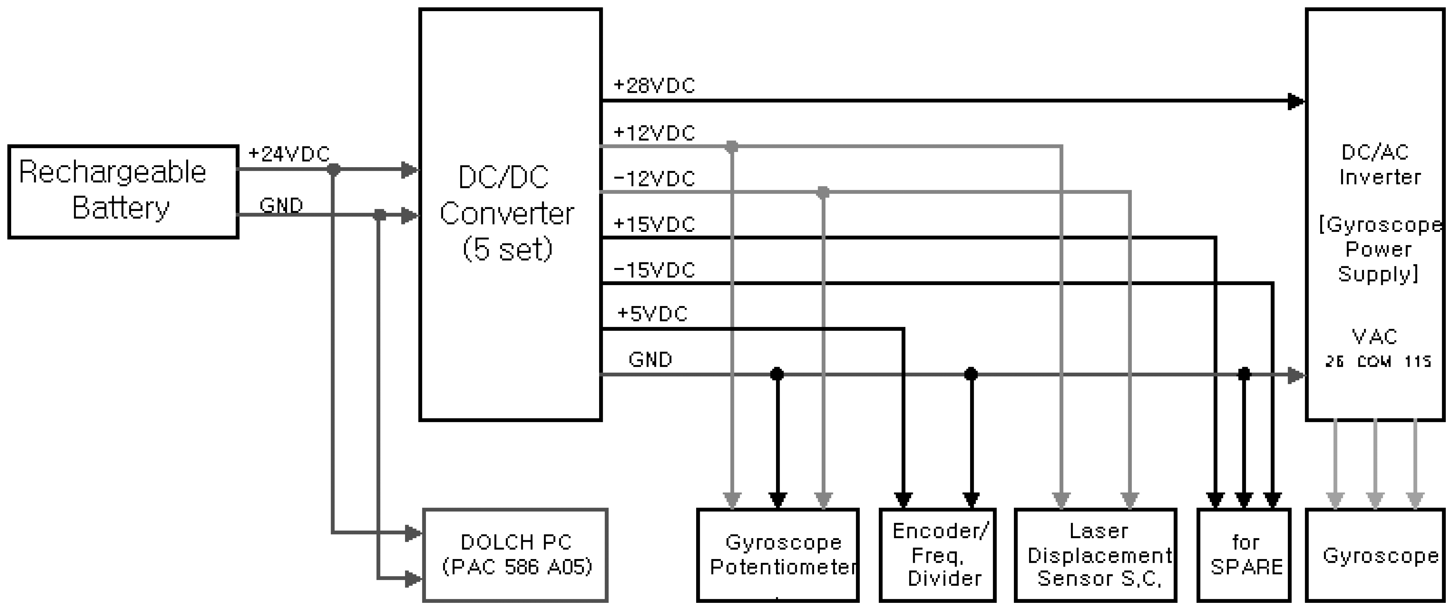
2.1. Composition of Hardware

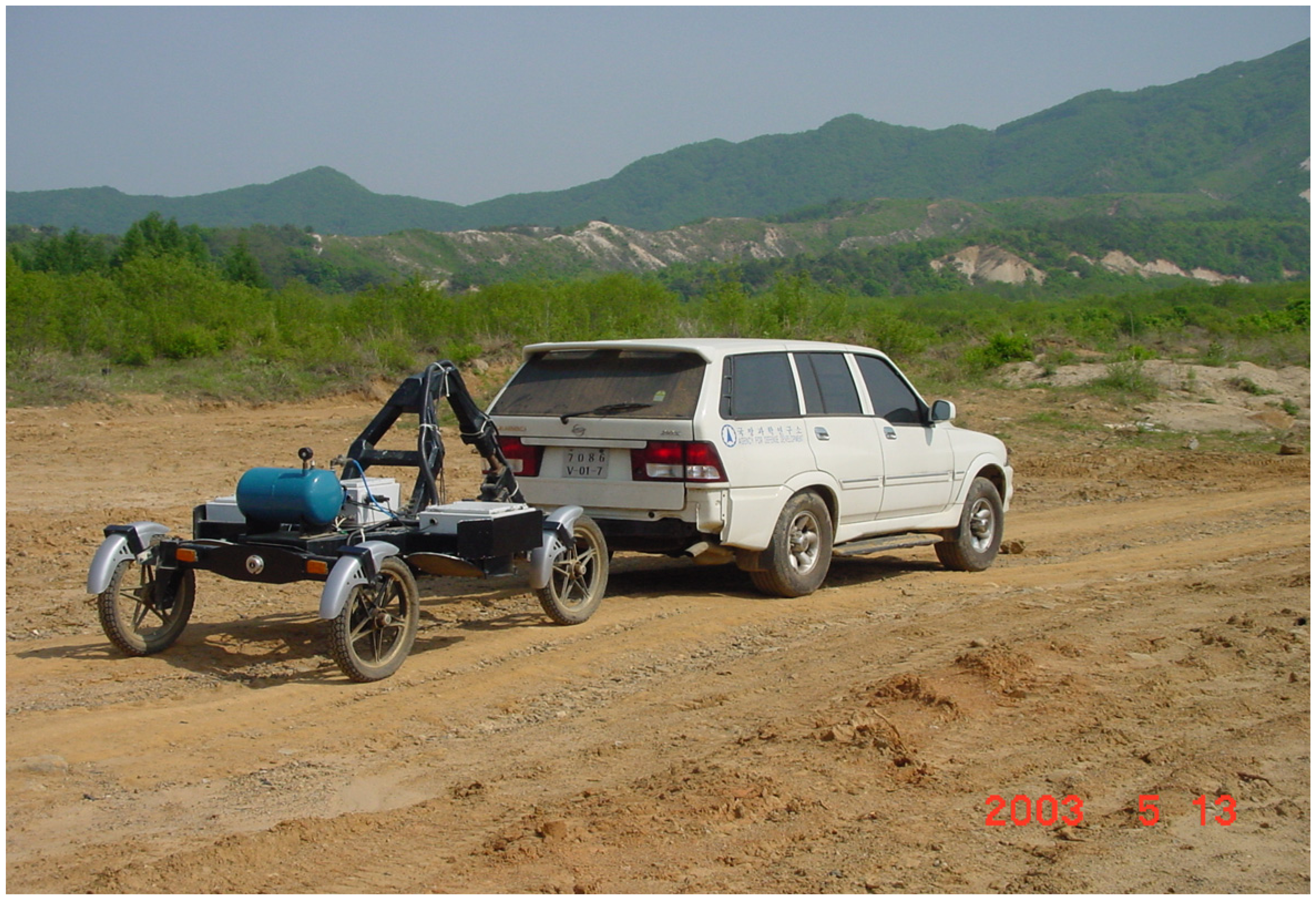
2.1.1 Trailer

The principal dimensions of the trailer were designed through the theoretical modeling analysis to measure the 20∼0.3m/cycle frequency range [8,9]. An overall length, wheel base, track and tire radius of the trailer are 3.1m, 1.2m, 1.8m and 0.287m, respectively. The trailer is composed of 4 wheels with two axles, and there are no compliant suspension components between the axles and the frame. The motion of the frame is described by two degree of freedom, yaw for the front axle and roll for the rear axle. A linkage between tractor and trailer is designed that the motion of tractor does not affect the trailer. While measuring, the air cylinder presses the trailer constantly to prevent from bouncing.

The vertical gyroscope is mounted on the trailer's midpoint to measure pitch and roll angle. The laser sensor is mounted on the left and right side of trailer respectively to measure vertical displacement. The wheel encoder on the rear right wheel measures moving distance. It has 3:1 gear ratio and resolving power of 6mm/pulse, so its sampling rate is 9.6cm.

2.1.2. Tractor

A Musso vehicle is modified as the tractor. Air compressor, data acquisition system (DAQ), amplifier and power supply unit are mounted on the vehicle. Air compressor is used to maintain continuous contact between the trailer and the ground and the pressure is set up to approximately 7kg/cm² through trial and error procedure at speed 5km/h.

The data acquisition system is a PC-based measuring system which is an industrial PC built in DAQ boards considering the environment of measurement

The power supply unit provides 24 VDC to the sensors on the trailer and the data acquisition system and amplifier on the tractor. Figure 2 shows the configuration of power system for instrumentation system.

2.2. Components of Software

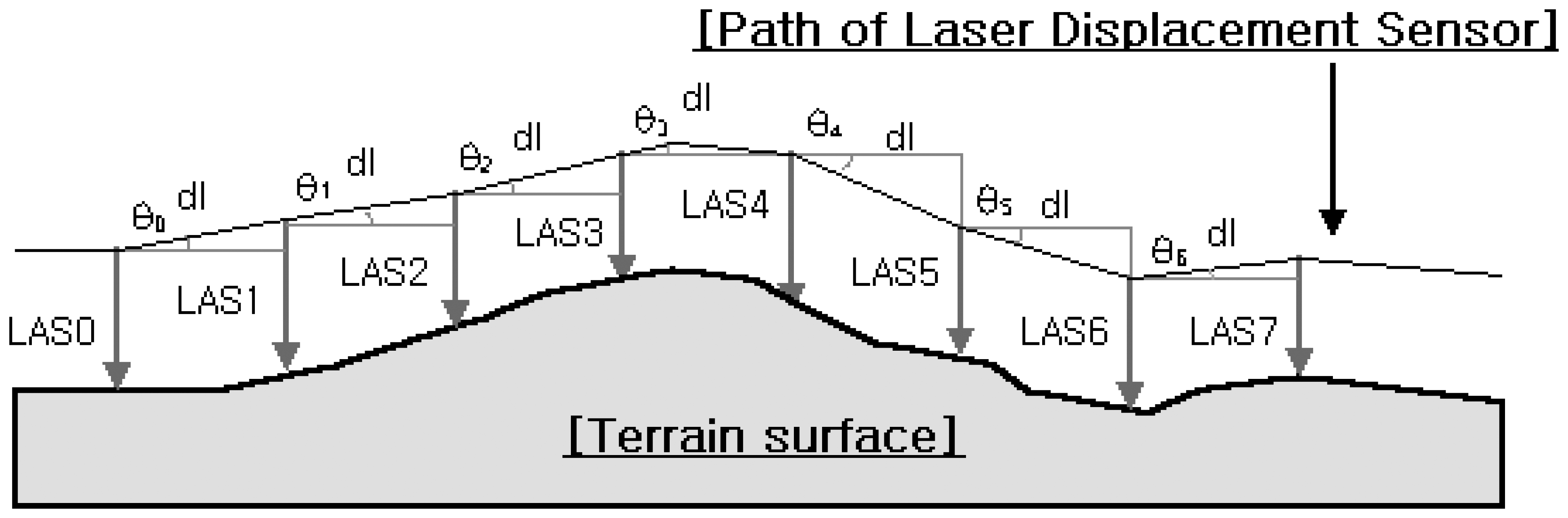
2.2.1. Generating Algorithm for profile

The Generating Algorithm reproduces a real profile using the pitch angle (θ), roll angle (ϕ) and vertical distance acquired from sensors on the trailer.

Eq.(1) is used to decide a moving trace of the trailer midpoint and Eq.(2) is used to get position coordinates of right and left laser sensors from the rolling motion of frame.

$$\begin{array}{c}{x}_{mp}(i+1)=\text{∑}_{i=0}^{N}cos{\theta }_{i}dl\\ y_{mp}(i+1)=\text{∑}_{i=0}^{N}sin{\theta }_{i}dl\\ y_l(i)=Y_{mp}(i)-\frac{W}{2}sin\varphi (i)\end{array}$$

(1)

$$y_r(i)=Y_{mp}(i)+\frac{W}{2}sin\varphi (i)$$

(2)

Here, x_mp is forward trace of the trailer midpoint and y_mp is vertical distance of the trailer.

y_r and y_l are right and left vertical position of laser sensors. The distance between laser sensor and trailer midpoint is $\frac{W}{2}=0.6\text{m}$.

$$\begin{array}{c}yl(i)=y_l(i)+LA{S}_l(i)\\ yr(i)=y_r(i)+LA{S}_r(i)\end{array}$$

(3)

Here, LAS_l and LAS_r are vertical displacements at the both sides of the trailer. yr and yl are the right and left terrain profiles, respectively. The trace of laser displacement sensor is shown in Figure 3.

$$\begin{array}{c}y{r}_R(i)=y_r(i)+\frac{LA{S}_r(i)}{cos\left|\theta (i)\right|cos\left|\varphi (i)\right|}\\ y{l}_R(i)=y_l(i)+\frac{LA{S}_l(i)}{cos\left|\theta (i)\right|cos\left|\varphi (i)\right|}\end{array}$$

(4)

$$\begin{array}{c}y{l}_m(i)=y{l}_R(i)+\left(x_r(i)-x(i)\right)\cdot tan(\theta (i))\\ y{r}_m(i)=y{r}_R(i)+\left(x_r(i)-x(i)\right)\cdot tan(\theta (i))\end{array}$$

(5)

Above equations are assumed that the laser sensor is vertical direction to the terrain surface, and it is necessary to correct the laser displacement sensor owing to the pitch and roll motion of the trailer. So the amended right and left profile are shown in Eq.(4).

The profiles for terrain surface can be acquired from the Eq.(4) but the sampling interval to the horizontal distance is not normalized. So it is necessary to normalize the data to correspond to sampling in equal increments of horizontal distance using the linear interpolation method such as Eq.(5).

yl_m and yr_m represent the linear interpolated final profile and x_r(i) is the normalized i-th sampling interval to the horizontal direction.

There are some errors owing to the approximate values in the Eq.5, but those are decreased when the sampling interval is smaller. The sampling rate applied this system, dl = 9.6cm, can be ignored considering the characteristics of terrain profile.

2.2.2. Analyzing Algorithms for profile severity

It is important that the profile acquired by the generating algorithm is managed to severity type. The algorithms to evaluate the severity comply with road grade classification according to ISO 8608 standard [7]. The road profile collected from the Eq.(5) goes through process of band pass filtering to get the frequency components of interesting band affecting suspension and frame of a vehicle.

ISO 8608 standard requires approximately one third sampling rate as the cutoff frequency to get over the aliasing and recommends 0.05cycle/m for detrending. Considering the sampling rate (9.6 cm) of the profilometer, that is about 0.05-3.46 cycle/m from the viewpoint of spatial frequency. It means that the interesting frequency band to the profilometer is 0.3-20 m/cycle.

Power Spectral Density (PSD) is used to evaluate the severity of road profile. The algorithms use the 5-th Butterworth filter, hanning window and PSD smoothing method [7,10] for signal processing. FFT block size is 1024 points.

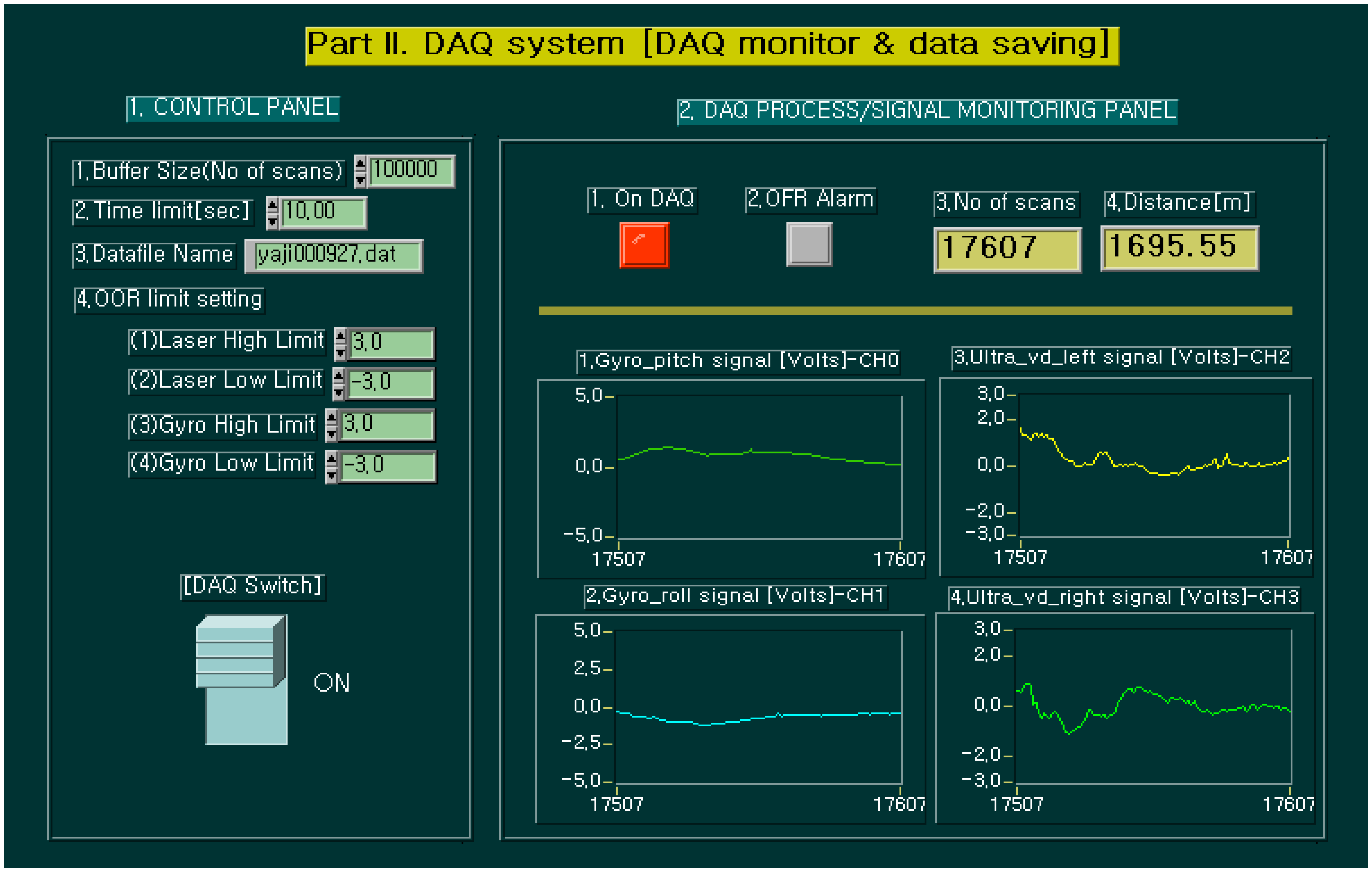
2.2.3. Operating Program

The operating program to get the road profile is developed using the LabView(ver.5.0). The program consists of measuring information part, data acquisition part and data confirmation part. In the measuring information part, measuring information, such as measuring date, road type, running direction, etc., is recorded and saved.

In the data acquisition part, measuring data is monitored and saved. The data confirmation part checks the normality of acquired data.

Figure 4 shows the data acquisition part. In this part, a tester can monitor the acquired data in real time and check the bad operation of sensors by lighting the OFR(out of range) warning lamp.

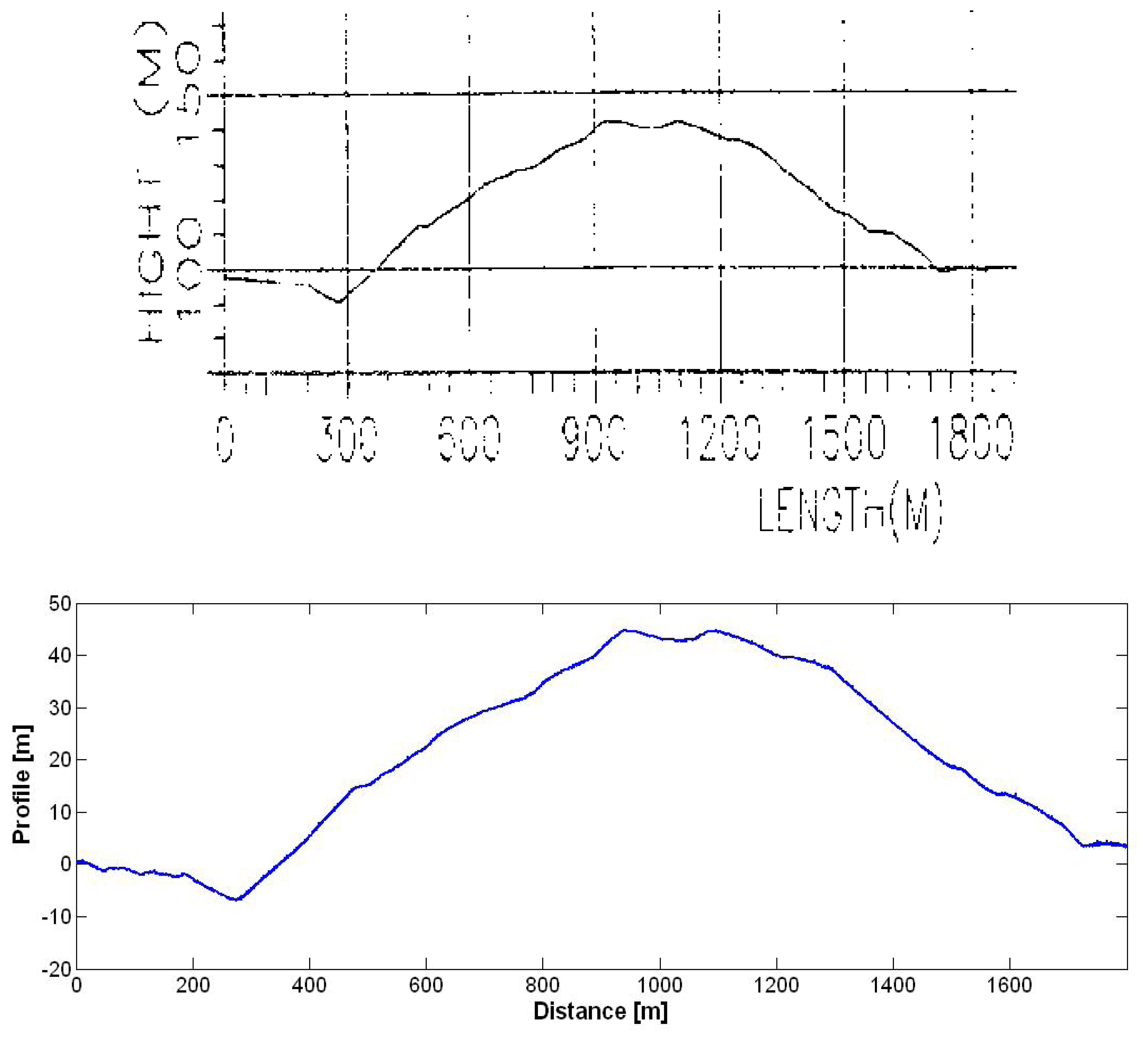
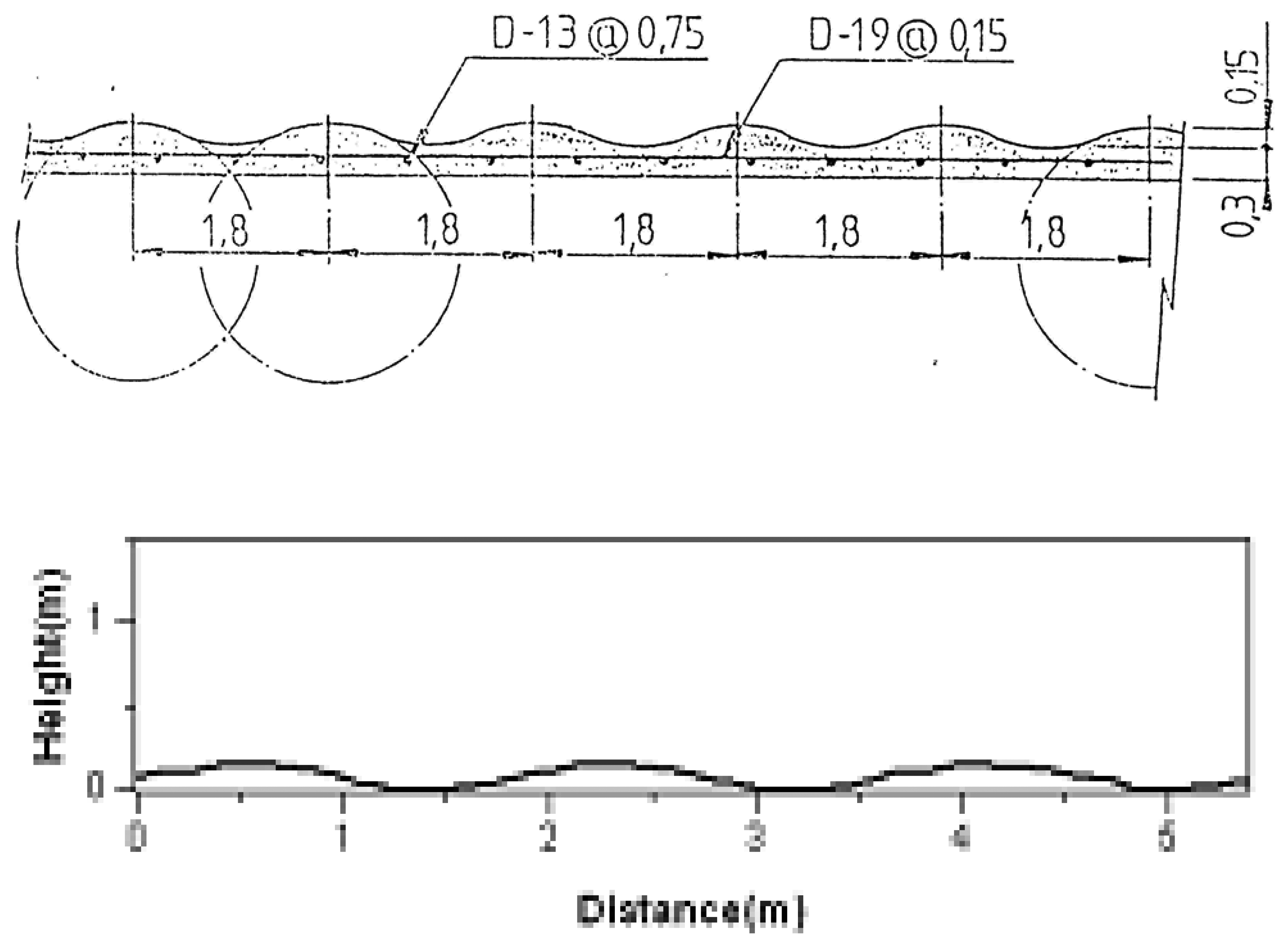
2.3. Proof of profilometer

To confirm the performance of profilometer, it is carried out to measure on the known road profiles that are gravel test course as shown Figure 5 and 6 inch washboard course as shown Figure 6.

Figure 5 shows the overall profile shape to the gravel test course at the CPG. The top plot is the shape acquired by the Road and Level Survey method and the bottom plot is the result acquired by the profilometer.

At a comparison between the two, the profile shapes are substantially the same.

Figure 6 shows the 6 inch washboard. To confirm the measuring ability for high frequency characteristics of the profilometer, the top plot is the drawing of 6 inch washboard and the bottom plot is the result acquired by the profilometer. Comparing between the two, it can be seen that the latter corresponds well to the former

3. Road Profile Characteristic Analysis and Severity Standardization

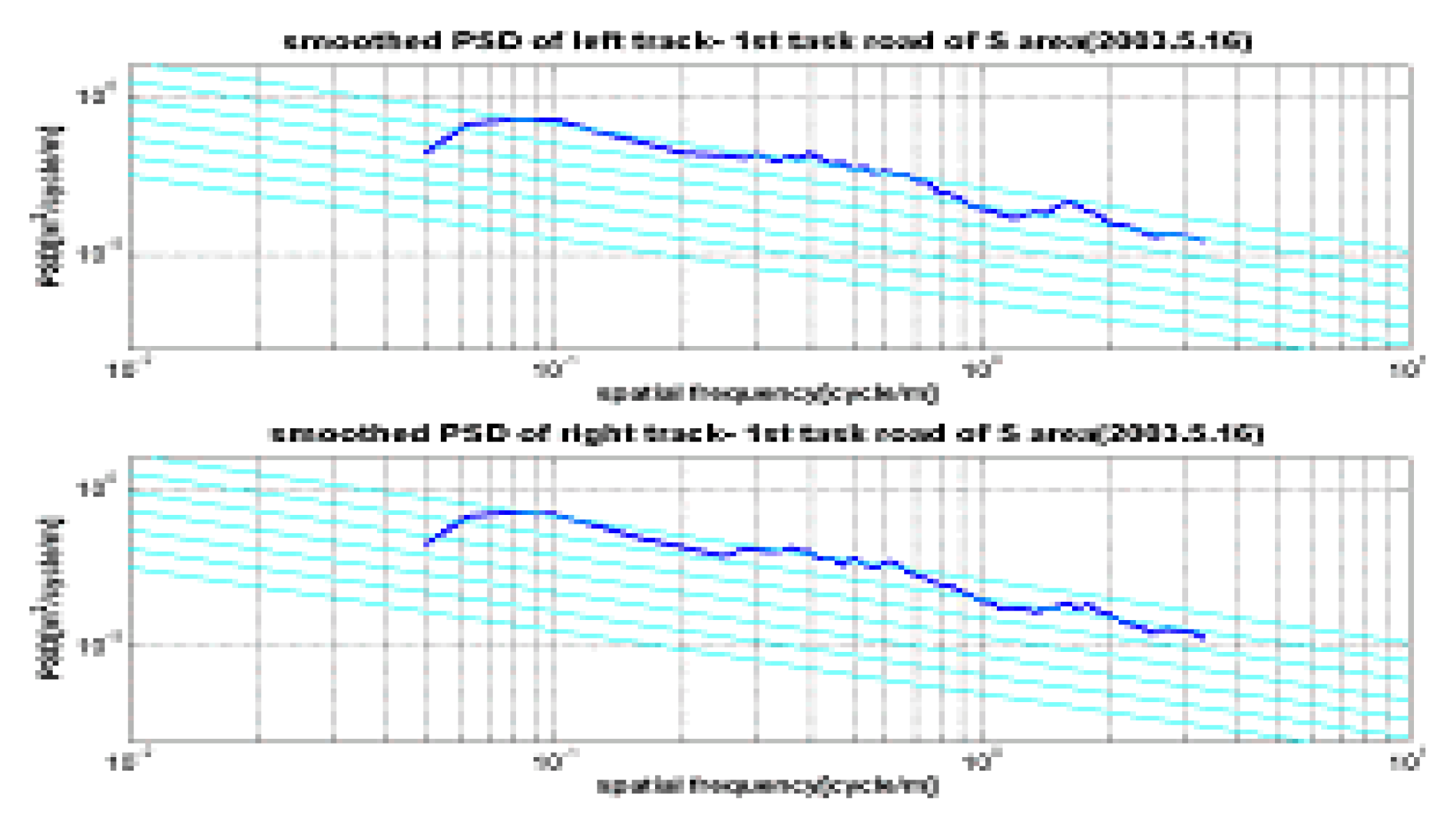
3.1. Road Classification in ISO 8608 standard

ISO 8608 standard classifies road severity to 8 classes(class A ∼ class H) using spatial frequency and octave band filtered displacement PSD, shown as

Table 1. Geometric mean and limits of the displacement PSD for different classes of roads as octave bands.

Road Class	Gd(nc) 10-6 m3	Octave centre spatial frequency, nc (cycle/m)
		0.0078	0.0156	0.0312	0.0625	0.125	0.25	0.5	1	2	4
A	Mean	2621	655	164	41.0	10.2	2.56	0.64	0.16	0.04	0.01
	Upper	5243	1311	328	81.9	20.5	5.12	1.28	0.32	0.08	0.02
B	Lower	5243	1311	328	81.9	20.5	5.12	1.28	0.32	0.08	0.02
	Mean	10486	2621	655	163.8	41.0	10.24	2.56	0.64	0.16	0.04
	Upper	20972	5243	1311	327.7	81.9	20.48	5.12	1.28	0.32	0.08
C	Lower	20972	5243	1311	327.7	81.9	20.48	5.12	1.28	0.32	0.08
	Mean	41943	10486	2621	655.4	163.8	40.96	10.24	2.56	0.64	0.16
	Upper	83886	20972	5243	1310.7	327.7	81.92	20.48	5.12	1.28	0.32
D	Lower	83886	20972	5243	1310.7	327.7	81.92	20.48	5.12	1.28	0.32
	Mean	167772	41943	10486	2621.4	655.4	163.84	40.96	10.24	2.56	0.64
	Upper	335544	83886	20972	5242.9	1310.7	327.68	81.92	20.48	5.12	1.28
E	Lower	335544	83886	20972	5242.9	1310.7	327.68	81.92	20.48	5.12	1.28
	Mean	671089	167772	41943	10485.8	2621.4	655.36	163.84	40.96	10.24	2.56
	Upper	1342177	335544	83886	20971.5	5242.9	1310.72	327.68	81.92	20.48	5.12
F	Lower	1342177	335544	83886	20971.5	5242.9	1310.72	327.68	81.92	20.48	5.12
	Mean	2684354	671089	167772	41943.0	10485.8	2621.44	655.36	163.84	40.96	10.24
	Upper	5368709	1342177	335544	83886.1	20971.5	5242.88	1310.72	327.68	81.92	20.48
G	Lower	5368709	1342177	335544	83886.1	20971.5	5242.88	1310.72	327.68	81.92	20.48
	Mean	10737417	2684354	671089	167772.1	41943.0	10485.76	2621.44	655.36	163.84	40.96
	Upper	21474834	5368709	1342177	335544.3	83886.1	20971.52	5242.88	1310.72	327.68	81.92
H	Lower	21474834	5368709	1342177	335544.3	83886.1	20971.52	5242.88	1310.72	327.68	81.92
	Mean	42949668	10737417	2684354	671088.6	167772.1	41943.04	10485.76	2621.44	655.36	163.84

[7]. It limits the displacements PSD for different classes of roads as function of the octave bands. ISO 8608 standard doesn't describe the configurations of each road classes, but it expresses that asphalted road belongs in class A. Tomoaki Mori et al. reported similar results for the concrete road using the profilometer developed by themselves [4,5]. Figure 7 gives classified concrete road measured by our profilometer, and this road was graded as A class by the classification method in ISO 8608.

3.2. Profile Measurement and Characteristic Analysis on Unpaved Road

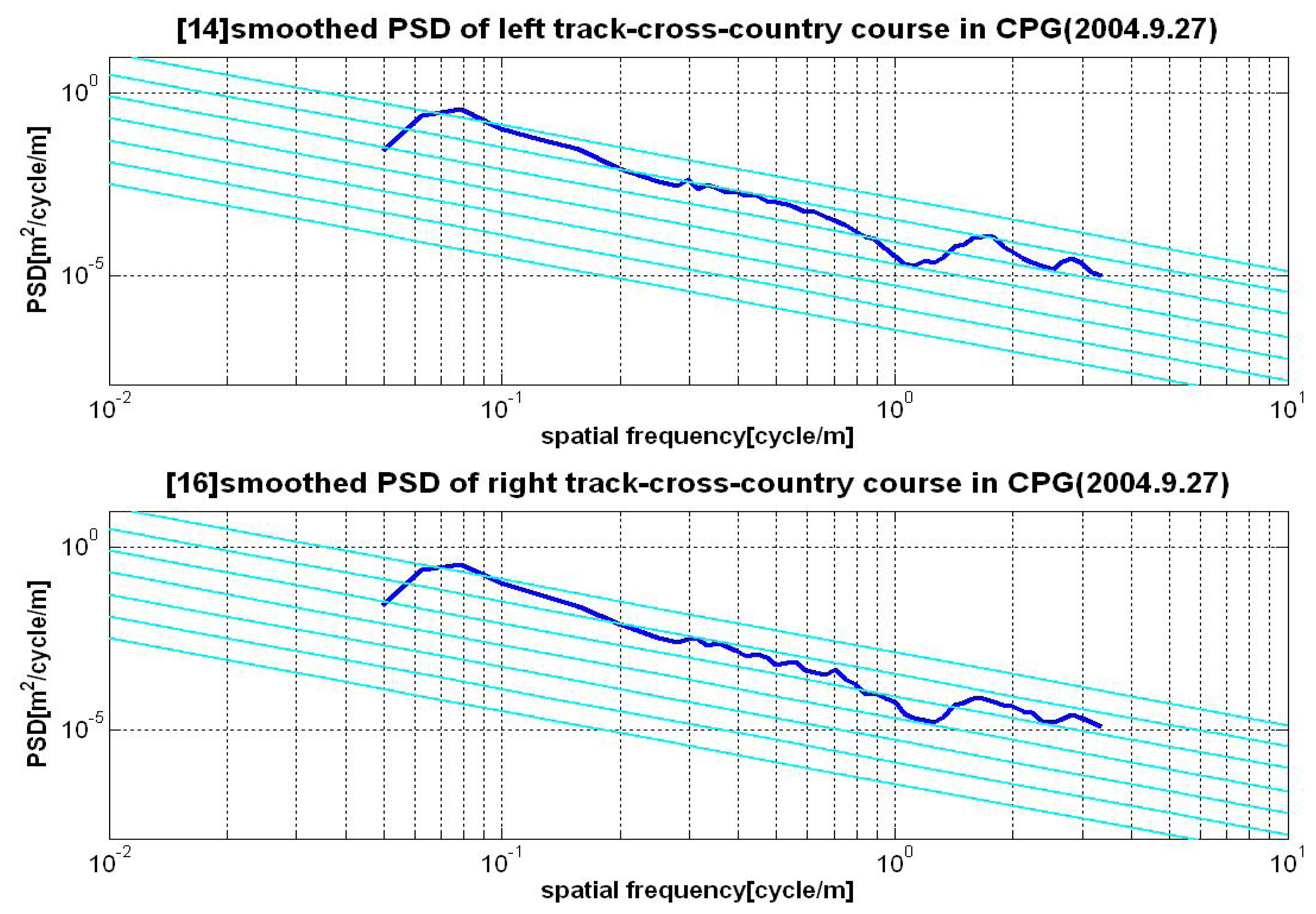
3.2.1. Cross-country Course in CPG

Figure 8 gives the profile data for left and right track of cross-country course in CPG. To extract interesting frequency ranges, we filtered the profile data for the ranges of 0.05∼3.46cycle/m. And we got road severity as shown in Figure 9, i.e. PSDs of left and right profiles of cross-country over ISO 8608 classification. Figure 9 gives that cross-country course in CPG is graded as class F and G in low frequency ranges (0.04∼0.3cycle/m), and graded as class F in middle frequency ranges (0.3∼1cycle/m), and graded as class E and F in high frequency ranges (1∼3.46cycle/m). From these results, we can find that road classification method suggested in ISO 8608 standard is an effective measure for comparing relative severity of roads.

3.2.2. Some Unpaved Roads

We measured road profiles for 23 unpaved roads all over the country in 2003. In this paper we only exhibit analyzed data for 4 roads whose practical usages are relatively frequent.

Figure 10 shows PSD of 3^rd task road in area M whose length is 2.2km. This road is graded as class F and G in low and middle frequency ranges, and graded as class E & F in high frequency ranges. Profile characteristic of this road is most similar to CPG cross-country course over all frequency ranges.

Figure 11 shows PSD of 1^st task road in area S whose length is 1.3km. This road is graded as class F and G in low and high frequency ranges, and graded as class G & H in middle frequency ranges. Profile characteristic of this road is severer than CPG cross-country course except low frequency ranges.

Figure 12 shows PSD of D task road in area Y whose length is 0.85km. This road is graded as class G in low and middle frequency ranges, and graded as class F & G in high frequency ranges. Profile characteristic of this road is severer than CPG cross-country course over all frequency ranges.

Figure 13 shows PSD of 1^st task road in area J whose length is 1.3km. This road is graded as class E and F in low and middle frequency ranges, and graded as class D & E in high frequency ranges. Profile characteristic of this road is less severe than CPG cross-country course over all frequency ranges.

3.2.3. Comparison of Road Profile Severity

Table 2. Comparison of road severity.

task road	Low Frequency.		Middle Frequency		High Frequency
cross-country	F	G	F		E	F
M-3rd area	F	G	F	G	E	F
S-1st area	F	G	G	H	F	G
Y-D area	G		G		F	G
J-1st area	E	F	E	F	D	E

summarizes severity comparisons of road profiles between cross-country course in CPG and 4 roads whose practical usages are relatively frequent. Comparison results show that 4 roads and cross-country course in CPG have similar characteristics in low frequency ranges, but 3 roads except the 1^st task road in J area is severer than cross-country course in middle and high frequency ranges.

3.3. Severity Standardization and Similarity Evaluation of Road Profile

3.3.1. Severity Standardization and Control Range Establishment of Road Profile

NATC(Nevada Automotive Test Center) in USA developed DFMV(Dynamic Force Measurement Vehicle) for profile measurement of unpaved road. And they have analyzed and controlled road severity using PSD of road profile. Controlling the road severity, they established severity standard firstly. They used the slope of profile PSD as severity standard. Second, they established the control ranges as ±3dB of the PSD slope. Using this standard and control ranges, they control road severity. I.e., if PSD slope goes out of control ranges, they make road more flat or bumpier to converge PSD slope into control ranges [8].

In this paper, we determined 52 PSD magnitudes at each spatial frequency by averaging acquired data from 2001 to 2003, as our severity standard. And we established control ranges as ±3dB of PSD magnitudes at each spatial frequency. This proposed method enables us that overall characteristics of road profiles can be maintained by controlling each PSD magnitude, instead controlling the overall slope of PSD. Figure 14 shows our severity standard and control ranges.

3.3.2. Evaluation on Similarity of Road Severity

To provide objectivity as a test course and to improve reliability of test results performed at CPG test course, we evaluated similarity of road severity between cross-country course in CPG and 4 roads whose practical usages are relatively frequent.

Generally, the PSD data reflects construction ratio of spatial frequency i.e. PSD pattern, and severity extent of road profile, i.e. magnitudes of PSD. So we propose similarity index composed of correlation index and inclusion index. Correlation index reflects PSD pattern i.e. characteristics of spatial frequency and inclusion index reflects the severity of road profile.

1)

Correlation Index of PSD Pattern

Correlation index is used for examining the relationship between two functions or two data. When correlation index is 1, two functions or data have totally same pattern, and is 0, they have totally different pattern, and is –1, they have totally opposite pattern.

Given data x and y as Eq.(6), correlation index between x and y, ρ_x,y can be obtained as Eq.(7). In Eq.(7), μ_x and σ_x, μ_y and σ_y are averages and standard deviations of data x and y.

$$\begin{array}{l}x=\left\{x_1,x_2,x_3,\cdot \cdot \cdot \cdot \cdot \cdot \cdot \cdot \cdot ,x_n\right\}\\ y=\left\{y_1,y_2,y_3,\cdot \cdot \cdot \cdot \cdot \cdot \cdot \cdot ,y_n\right\}\end{array}$$

(6)

$$\begin{array}{c}{\rho }_{x,y}=\frac{\mathit{\text{Cov}}(X,Y)}{{\sigma }_x•{\sigma }_y},-1\le {\rho }_{x,y}\le 1\end{array}$$

(7)

$$\begin{array}{c}\text{with}\mathit{\text{Cov}}(X,Y)=\frac{1}{n}\text{∑}_{j=1}^n\left\{(x_j-{\mu }_x)(y_j-{\mu }_y)\right\}\end{array}$$

In the case that data is PSDs of road profiles, correlation index ρ_x,y has nothing to do with PSD magnitudes of road profiles, but it is closely related with PSD patterns or PSD shapes.

2)

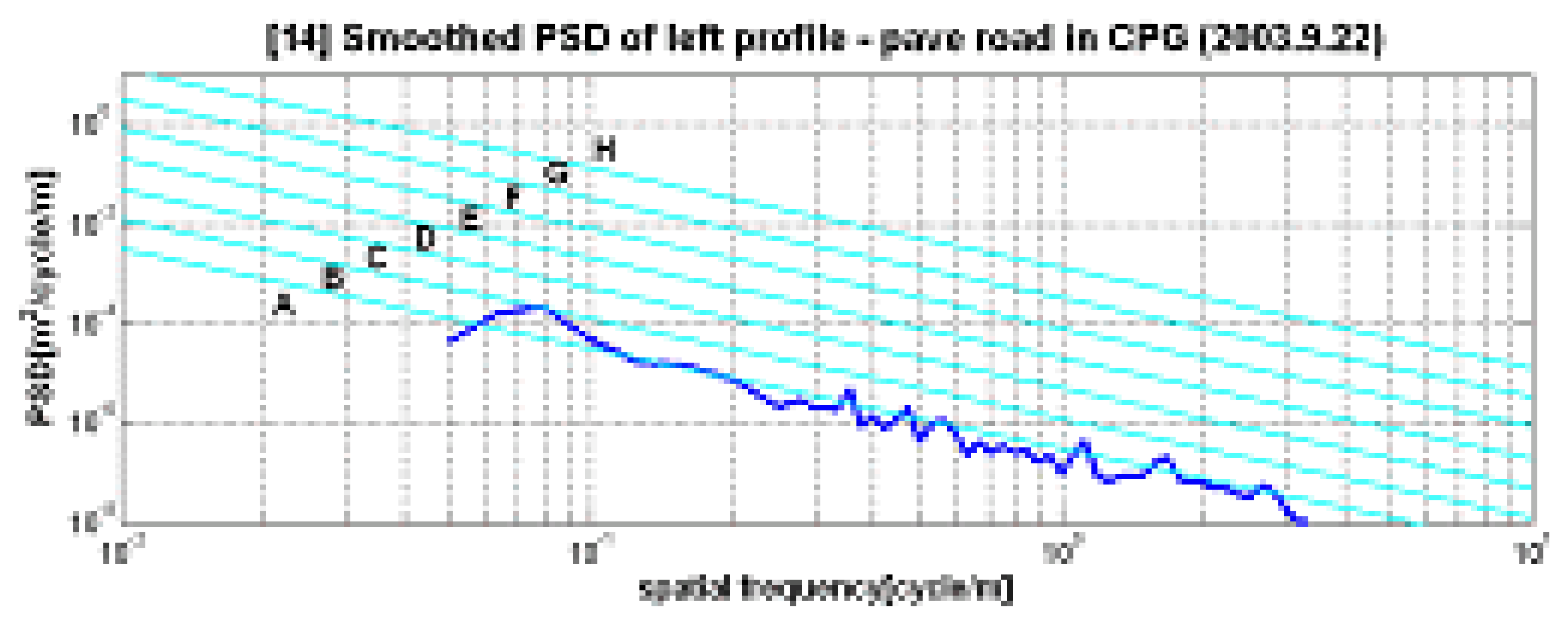
Inclusion Index for Control Ranges

To evaluate the similarity of road profile characteristics, we should consider not only PSD pattern but also PSD magnitude. So we defined inclusion index for control ranges, γ_x,y as Eq.(8) to compare magnitudes of profile PSD, between arbitrary unpaved road and cross-country course in CPG. γ_x,y is a simple rate whether each PSD magnitude at 52 spatial frequency is included in the established control ranges of cross-country course in CPG or not.

$${\gamma }_{x,y}=\frac{n_{x,y}}{52}$$

(8)

Here, n_x,y is the numbers of profile PSD values of arbitrary roads (y) which are included in the PSD control ranges of the cross country (x) in the CPG.

Figure 15 shows PSD of the cross-country measured at 3^rd quarter of 2003, and it gives that 4 of PSD magnitudes at spatial frequency (1.0, 1.0595, 1.1225, and 2.8784cycle/m) mark as ■, exceed the control ranges. So the inclusion comes to 0.9985 in this case.

3)

Similarity Index

To evaluate the similarity of road profile characteristics, we defined similarity index, δ_x,y as Eq.(9).

$${\delta }_{x,y}=\nu \times {\rho }_{x,y}+(1-\nu )\times {\gamma }_{x,y}$$

(9)

Here, ν is a weighting factor, and we applied ν as 0.3 subjectively. This means that we put higher value on inclusion index than correlation index determined by PSD pattern.

3.3.3. Results of Similarity Evaluation

Figure 16 shows profile PSDs of 1^st and 3^rd task road in area M over the control ranges of cross-country course in CPG. For the case of 1^st task road, ρ_x,y was 0.961, and any values of PSD magnitudes don't go out of control ranges, i.e. γ_x,y was 1.0. So similarity index δ_x,y was 0.988, and this was the most similar road with cross-country course in CPG, among the 23 roads that we have measured their profiles. In the case of 3^rd task road, the ρ_x,y was 0.971 and this was the most similar case in PSD pattern aspect. 5 values of PSD magnitudes go out of control ranges, so γ_x,y was 0.90, and similarity index δ_x,y was 0.924.

Figure 17 shows profile PSDs of 1^st task road in area S and D task road in area Y over the control ranges of cross-country course in CPG. PSD patterns are similar on the whole, but lots of PSD values exceed the upper limit of control range. So the similarity indices were 0.509 and 0.378.

Figure 18 shows the results of 1^st task road in area J and 2^nd task road in area D.

Table 3. Comparison of Similarity Degree.

Task Road Name	ρx,y	γx,y	δx,y
M-1st area	0.961	1.000	0.988
M-3rd area	0.971	0.904	0.924
S-1st area	0.935	0.327	0.509
Y-D area	0.902	0.154	0.378
J-1st area	0.942	0.673	0.754
D-2nd area	0.956	0.923	0.933
average	0.945	0.664	0.748
average PSD's	0.960	0.769	0.826

summarizes correlation indices, inclusion indices, and similarity indices for 6 task roads all over the country. The average of similarity indices was 0.748, but the similarity index on averaged PSD values at each spatial frequency over 6 task roads, was 0.826. Similarity index were 0.748 and 0.826, and both values can be interpreted that road profile characteristic of cross-country course whose control ranges are defined as in this paper, is very similar that of compared roads where automotive equipments run over very frequently.

4. Road Severity Management Algorithm using Neural Network

Even though the severity management range of test courses is standardized precisely, systematic technique for road management is needed in order to carry out management of the road profile effectively.

4.1. Evaluation of PSD effect

We have a limitation to prove the PSD effect by realizing practical road according to the various period, amplitude and number of profile. Thus, simulation program is built in the direction of the evaluation of PSD effect using generated profile by computer. This program calculates the smoothed PSD as same process as the ISO 8608 standard. That is, as a case in point, Figure 19 shows the sine wave with period 1.06m/cycle, amplitude 0.15m and number 6 on the flat virtual test course and the smoothed PSD for applied sine wave.

As it remarked above, the results for evaluation of PSD effect consist of the training sets for Road Severity Management Algorithm using Neural Network. The quantity of PSD effect evaluation is 468(52 kinds of period × 3 kinds of amplitude × 3 kinds of sine wave number).

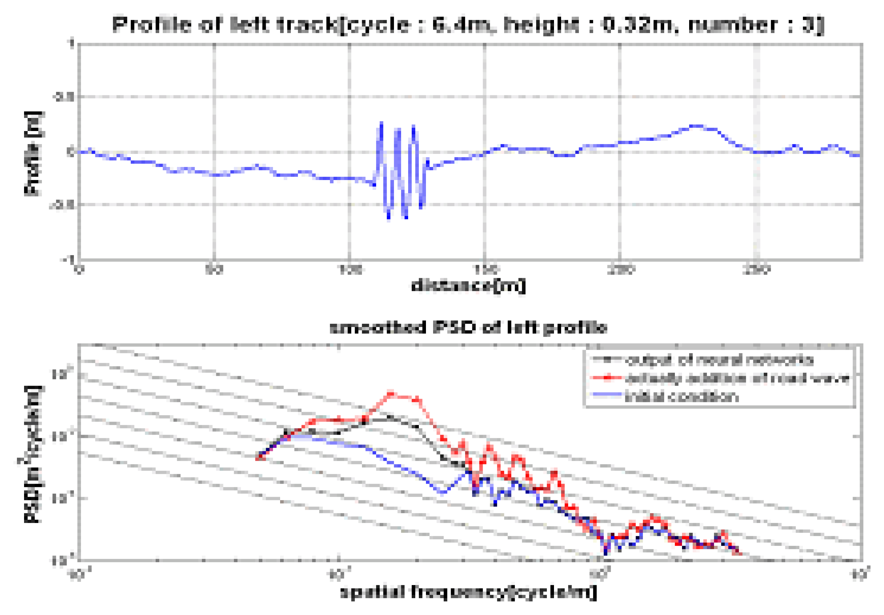
4.2. Development of Road Profile Severity Management Algorithm

Road Severity Management Algorithm can be introduced to generate needed road profile so much that PSD values break away from severity management range in each spatial frequency.

4.2.1. Architecture

In general, the decisive method of neuron number for hidden layer is studied in neural network. But optimized neuron number is determined by the trial and error procedure [10]. Figure 20 shows a three-layer neural network that takes various PSD values break away from severity management range in each spatial frequency as inputs. Its input layer has 52 nodes and one bias node while the output layer has 104 nodes. In between the two layers, there are 300 hidden nodes. Each node has a unipolar sigmoid function and the weight of each connection is updated by the momentum back propagation algorithm.

4.2.2. Applied Learning Rule

In this study, applied learning rule in the Road Severity Management Algorithm is the Momentum Back-propagation Algorithm in order to prevent a local minimum and reduce the learning time. The purpose of the momentum method is to accelerate the convergence of the error back-propagation learning algorithm.

In general, the incremental learning of the weight matrix in error back-propagation algorithm is determined by learning rate α and error value δ of each layer. For large learning constants, the learning speed can be drastically increased. However, the learning may not be exact, with tendencies to overshoot, or it may never stabilize at any minimum. Even though the simple gradient descent can be efficient, the error back-propagation algorithm involves supplementing the current weight adjustment with a fraction of the most recent weight adjustment. Thus the choice of the learning constant depends strongly on the class of the learning problem. The Momentum constant β is a user-selected positive momentum constant and chosen between 0.1 and 0.8 typically.

In this study, α and β are made choice of 0.7 and 0.5 respectively. And, the training cycle is completed if learning is exceeded the 200,000 iteration limit or normalized average error rate E_max falls under 0.3.

The algorithm of error back-propagation training is given below.

• Step 1. Weights w and v are initialized at small random values (-0.5∼0.5); w is (k × j), v is (j × i). And Error value E is initialized 0.
• Step 2. Training step starts here. Input is presented and then the layer's outputs are computed such as Eq.(10). Applied λ=1 for unipolar sigmoid function. And P is applied 208 which is the number of training pairs.
  $$\begin{array}{l}\begin{array}{l}NE{T}_y=z_k{v}_k^T\hfill \\ y=f(NE{T}_y)=\frac{1}{1+exp(-\lambda NE{T}_y)}\hfill \\ NE{T}_o=y_k{w}_k^T\hfill \\ o=f(NE{T}_o)=\frac{1}{1+exp(-\lambda NE{T}_o)}\hfill \end{array}\hfill \end{array}$$

  (10)
• Step 3. Error value E is computed such as Eq.(11)
  $$E\leftarrow E+\frac{1}{2}{(d_k-o_k)}^2$$

  (11)
• Step 4. For activation function of an neuron is used the unipolar continuous sigmoid function, error signal vectors δ_ok and δ_yj of both layers are computed such as Eq.(12) and Eq.(13).
  $$\begin{array}{c}{\delta }_{ok}=(d_k-o_k)f\text{'}(NE{T}_y)=o_k(d_k-o_k)(1-o_k)\\ *f\text{'}(NE{T}_y)=o_k(1-o_k)\end{array}$$

  (12)

  $$\begin{array}{c}{\delta }_{yj}=w_j^t{\delta }_{ok}f\text{'}(NE{T}_y)=y_j(1-y_j)\text{∑}_{k=1}^K{\delta }_{ok}{w}_{kj}\\ *f\text{'}(NE{T}_y)=y_j(1-y_j)\end{array}$$

  (13)
• Step 5. Output layer weights are adjusted such as Eq.(14).
  $$w^{k+1}=w^k+\mathrm{\Delta }{w}^k=w^k+\alpha {\delta }_o{y}^k+\beta \mathrm{\Delta }{w}^{k-1}$$

  (14)
• Step 6. Hidden layer weights are adjusted such as Eq.(15).
  $$v^{k+1}=v^k+\mathrm{\Delta }{v}^k=v^k+\alpha {\delta }_y{z}^k+\beta \mathrm{\Delta }{v}^{k-1}$$

  (15)
• Step 7. If p < P then p ← p + 1, q ←q + 1 and go to step 2; otherwise, go to step 8.
• Step 8. The training cycle is completed.
  For E < E_max terminate the training session. Output weights w, v, q, E.
  If E > E_max, then E ← 0, q ← 1 and initiate the new training cycle by going to step 2.

By this way, learning is executed and completed at 136,000 iterations approximately with 208 data set obtained from the simulation, as shown in Figure 21. That is, the average error rate E_max is below 0.3(30%) on that point.

4.3. Experimental Results and Discussion

As it was remarked above, Road Severity Management Algorithm using Neural Network has been conducted to learn with 208 among the 468 data set obtained from the PSD effect evaluation. In order to prove the effectiveness of this developed program, unpaved course about 300m length was leveled by the excavator. After the unpaved course leveled, Figure 22 shows the profile and PSD using the profilometer for initial condition of leveled unpaved course.

The purpose of experiment such as Figure 23 is to compare developed algorithm output with construction result on the unpaved course about PSD for spatial frequency of low range. That is, in order to increase the PSD 0.05m³/cycle for period 6.4m/cycle, the sine wave with amplitude 0.32m and number 3 obtained from this program. But, the amplitude of constructed sine wave by the excavator is close to 0.5m.

Table 4. Comparison of PSD for low frequency.

Spatial frequency (m/cycle)	Object value (m3/cycle)	Neural output (m3/cycle)	Measuring value (m3/cycle)
0.1250		0.03	0.04
0.1563	0.05
0.1575		0.04	0.24
0.1984		0.02	0.15

shows the PSD value with each other.

The purpose of experiment such as Figure 24 is to compare developed algorithm output with construction result on the unpaved course about PSD for spatial frequency of medium range. That is, in order to increase the PSD 0.001m³/cycle for period 2.5m/cycle, the sine wave with amplitude 0.18m and number 2 obtained from this program. But, the amplitude of constructed sine wave by the excavator is close to 0.3m.

Table 5. Comparison of PSD for medium frequency.

Spatial frequency (m/cycle)	Object value (m3/cycle)	Neural output (m3/cycle)	Measuring value (m3/cycle)
0.3969		0.001	0.004
0.4000	0.001
0.4205		0.001	0.003
0.4455		0.001	0.003

shows the PSD value with each other.

In the same manner, the purpose of experiment such as Figure 25 is to compare developed algorithm output with construction result on the unpaved course about PSD for spatial frequency of high range. That is, in order to increase the PSD 0.00003m³/cycle for period 0.4m/cycle, the sine wave with amplitude 0.05m and number 10 obtained from this program. But, this case was constructed higher than output profile of developed program.

Table 6. Comparison of PSD value for high frequency.

Spatial frequency (m/cycle)	Object value (m3/cycle)	Neural output (m3/cycle)	Measuring value (m3/cycle)
2.3784		0.00002	0.00001
2.5000	0.00003
2.5198		0.00003	0.00011
2.6697		0.00002	0.00017

shows the PSD value with each other.

By executing these experiments, the Road Severity Management Algorithm using Neural Network was verified effectively in acquiring road profile needed, which does not depend on human expertise and saves much on the trial-and-error procedure. But, the construction technique by excavator is difficult to realize.

5. Summary and Conclusions

This paper has presented the development and evaluation of the road profile measurement system to maintain severity for unpaved test courses by combining the principle ISO 8608 standard and neural network. The major conclusions derived from this research are delineated below.

1)

The system composed of profilometer and data analysis program according to the ISO 8608 standard process is very effective in measurement and analysis for unpaved road profile.

2)

The severity of road including the cross-country test course in CPG and the task road in Army Operating Area has been classified into eight grades according to the criterion of ISO 8608 standard.

3)

By introducing the similarity index to evaluate the quantified profile characteristics between roads, the reliability of the endurance test for development vehicle of military is enhanced.

4)

The Road Severity Management Algorithm including the severity standardization can be used to implement the road management in order to maintain the severity level.

References and Notes

- Connon, W. H. Determining Vehicle Sensitivity to Changes in Test - Course Roughness. IEST 46th Annual Technical Meeting and Exposition. 2000, 30–37. [Google Scholar]
- Dodds, C. J.; Robson, J. D. The description of the road profile roughness. Journal of Sound and Vibration 1973, 31, 175–183. [Google Scholar]
- Min, B.H.; Jeong, W.U. Design Method of Test Road Rrofile for Vehicle Accelerated Durability Test. Journal of KSAE 1994, 2(1), 128–141. [Google Scholar]
- Castaldo, P.D.; Allred, J.A.; Reil, M.J. Terrain Profilometer.; Technical Report; Aberdeen Proving Ground of US Army, 2000. [Google Scholar]
- Tomoaki, M.; Seikichi, N.; Kanagawa, K.; Inoue, Y.; Yoshioka, K.; Matsushita, Y.; Shimura, A. Study on the characteristics of terrain profiles to develop the tracked vehicle suspension.; Technical Report; Technical Research and Development Institute in Japan Defense Agency, 1992. [Google Scholar]
- La Barre, R.P.; Forbes, R.T.; Andrew, S. The Measurement and Analysis of Road Surface Roughness.; Technical Report; Motor Industry and Research Association, 1969. [Google Scholar]
- ISO. Mechanical Vibration - Road Surface Profiles - Reporting of Measured Data. ISO 8608:1995(E). 1995.
- Ashmore, S.C.; Hodges, H.C. Dynamic Force Measurement Vehicle (DFMV) and Its Application to Measuring and Monitoring Road Roughness.; Vehicle, Tire, Pavement Interface, ASTM STP 1164 American Society for Testing and Materials: Philadelphia; pp. 69–96. 1992. [Google Scholar]
- Xu, D.M.; Mohamed, A.M.O.; Yong, R.N.; Caporuscio, F. Development of a Criterion for Road Surface Roughness Based on Power Spectral Density Function. Journal of Terramechanics 1992, 29, 477–486. [Google Scholar]
- Mitra, S.; Pal, S.K. Self-Organizing Neural Network As A Fuzzy Classfier. IEEE Trans. on Sys., Man. and Cybern. 1994, 24(3), 385–398. [Google Scholar]