From Maxwell’s Equations to Polarimetric SAR Images: A Simulation Approach

Abstract
:1. Introduction
2. Electromagnetic Model
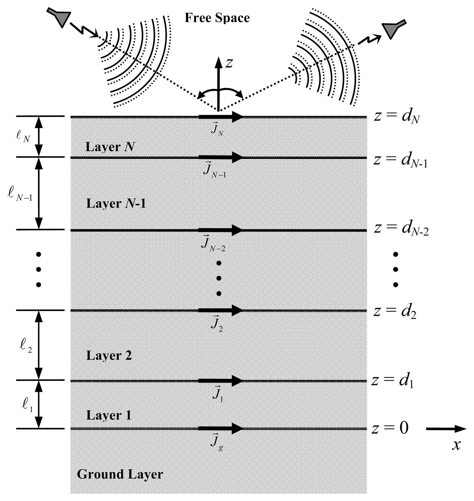
2.1. Electromagnetic Fields in the Structure
 nϑ (kx,ky) are
 nϑ (kx,ky) the amplitudes of the transformed field components, kx and ky are the spectral variables, γn is the propagation constant in the n-th layer, ϑ = x, y or z, and Im( ) means the imaginary-part function. The τ variable, which defines the wave propagation direction, can assume values 1 or 2. Only the former value, representing propagation in the positive-z direction, occurs in the upper layer (free space). For the ground layer, on the other hand, τ equals 2, i.e., a wave propagating in the negative-z direction. For the confined layers, however, both values of τ will occur.
2.2. Moment Method - MoM
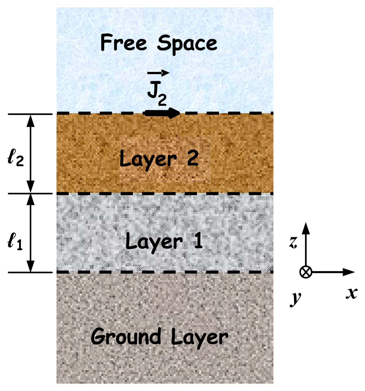
2.3. Four-Layer Structure
0z (kx, ky) and
0z (kx, ky) are necessary to compute the electric far field, as shown in (20). In this particular case, the surface current along the y direction is neglected since the dipole width is considered to be very thin. Thus only the
matrix, represented by [Zpm], involving the Green's function
, needs to be evaluated. After the aforementioned mathematical simplifications, the [Zpm] matrix becomes
3. Polarimetric SAR Image Simulation
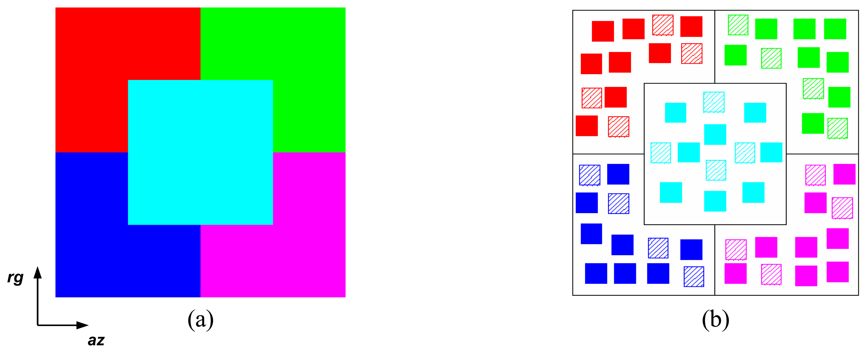
3.1. Simulated Images
4. Image Analysis
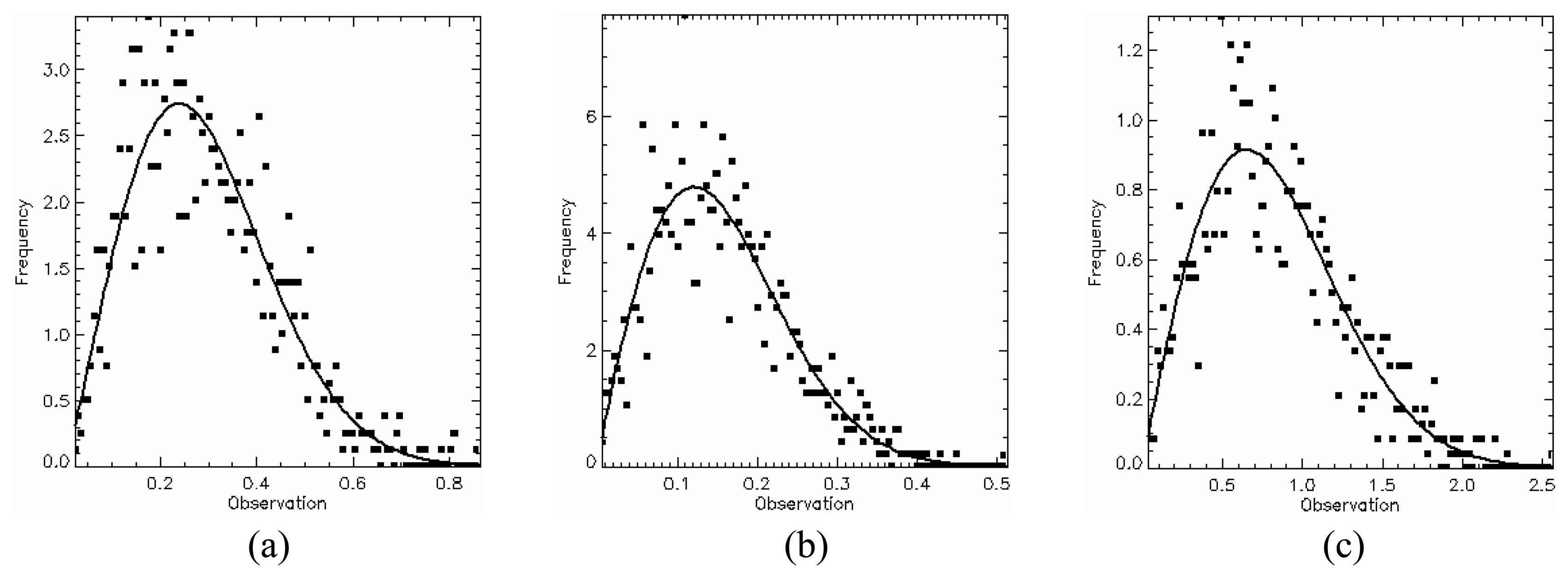
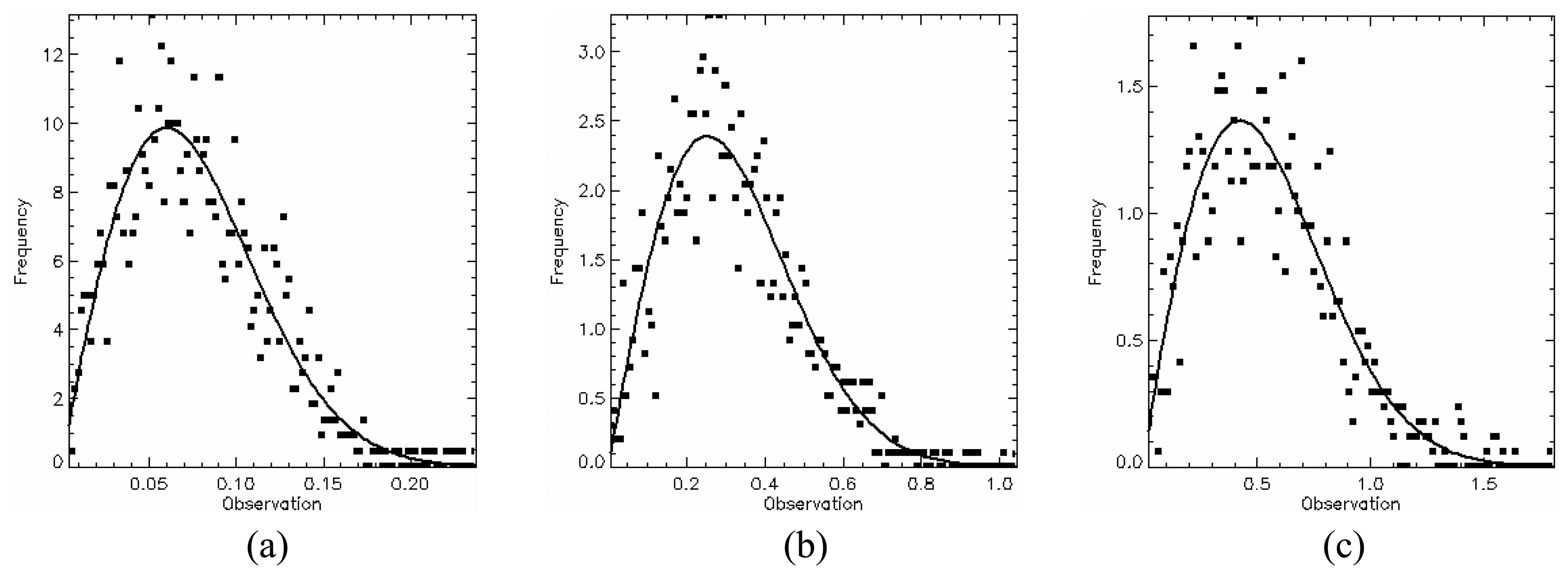
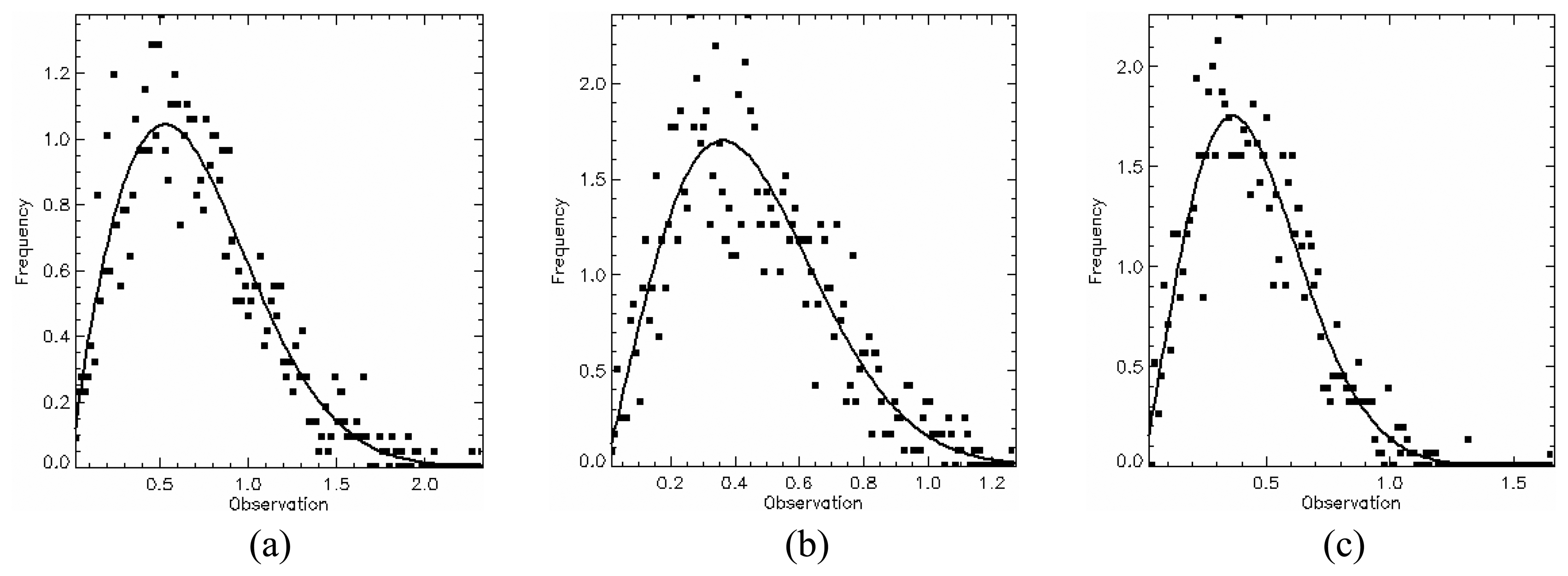
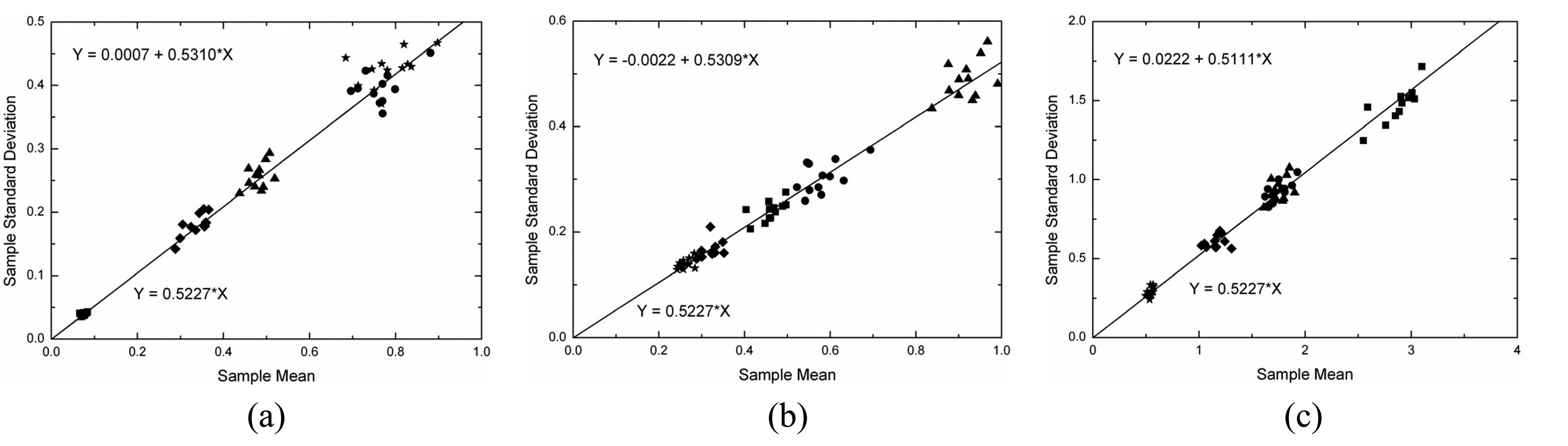
4.1 Amplitude Data
4.2 Polarimetric Data
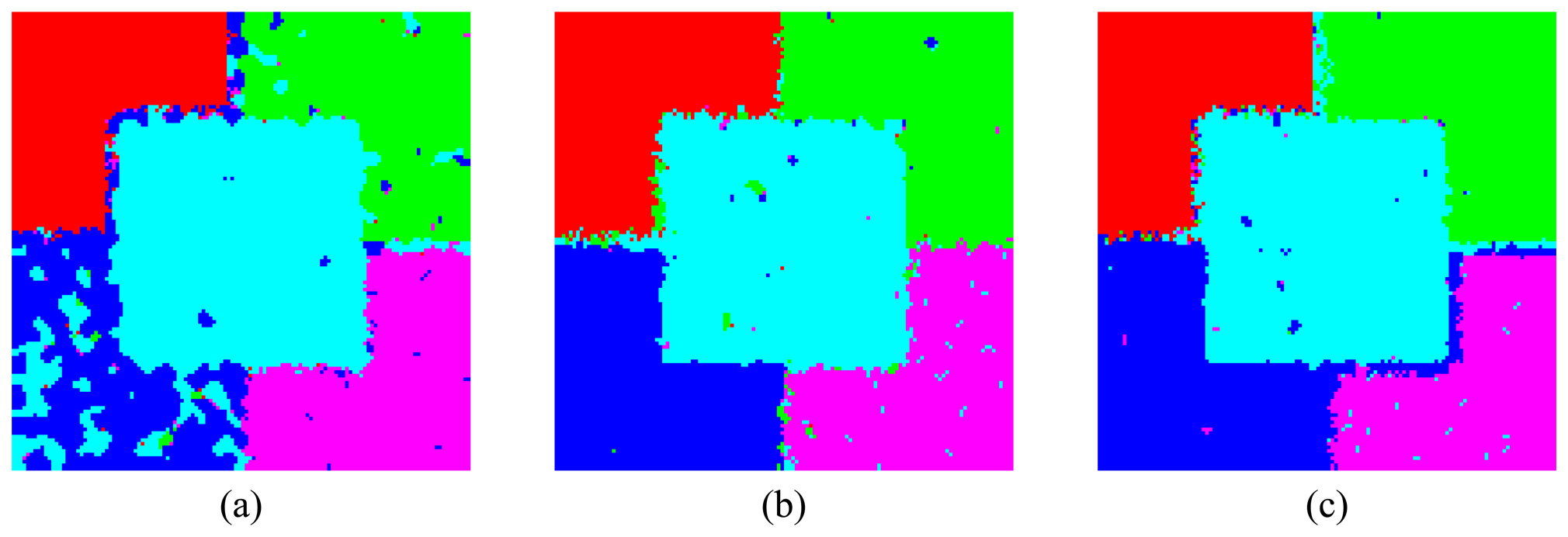
4.3 Data Classification
5. Conclusions
Acknowledgments
References and Notes
- Lucca, E.V.D.; Freitas, C.C.; Frery, A.C.; Sant'Anna, S.J.S. Comparison of SAR segmentation algorithms. In Segunda Jornada Latino-Americana de Sensoriamento Remoto por Radar: Técnicas de Processamento de Imagens.; Santos, São Paulo, Sept. 1998. [Google Scholar]ESA Workshop Proceedings; 1999; pp. 123–130, ESA SP-434.
- Moschetti, E.; Palacio, M.G.; Picco, M.; Bustos, O.H.; Frery, A.C. On the use of Lee's protocol for speckle-reducing techniques. Lat. Am. Appl. Res. 2006, 36, 115–121. [Google Scholar]
- Gambini, J.; Mejail, M.; Jacobo-Berlles, J.; Frery, A.C. Accuracy of edge detection methods with local information in speckled imagery. Stat. Comput. 2008, 18, 15–26. [Google Scholar]
- Frery, A. C.; Müller, H. J.; Yanasse, C. C. F.; Sant'Anna, S. J. S. A model for extremely heterogeneous clutter. IEEE T. Geosci. Remote Sens. 1997, 35, 648–659. [Google Scholar]
- Sant'Anna, S.J.S.; Lacava, J.C.S.; Fernandes, D. A useful tool to simulate polarimetric SAR images. Eleventh URSI Commission F Triennial Open Symposium on Radio Wave Propagation and Remote Sensing. Anais., Rio de Janeiro, RJ, Brazil, 30 Oct. / 02 Nov., 2007.
- Singh, D.; Dubey, V. Microwave bistatic polarization measurements for retrieval of soil moisture using an incident angle approach. J. Geophys. Eng. 2007, 4, 75–82. [Google Scholar]
- Sarabandi, K.; Nashashibi, A. A novel bistatic scattering matrix measurement technique using a monostatic radar. IEEE T. Antenn. Propag. 1996, 44, 41–50. [Google Scholar]
- Lacava, J.C.S.; Proaño De la Torre, A.V.; Cividanes, L. A dynamic model for printed apertures in anisotropic stripline structures. IEEE T. Microw. Theory 2002, 50, 22–26. [Google Scholar]
- Newman, E.H.; Forrai, D. Scattering from microstrip patch. IEEE T. Antenn. Propag. 1987, AP-35, 245–251. [Google Scholar]
- Collin, R.E.; Zucker, F.J. Antenna Theory: Part 1; McGraw-Hill Book Company: New York, 1969. [Google Scholar]
- Marin, M.A.; Barkeshli, S.; Pathak, P.H. On the location of proper and improper surface wave poles for the grounded dielectric slab. IEEE T. Antenn. Propag. 1990, 38, 570–573. [Google Scholar]
- Sant'Anna, S.J.S.; Pereira, C.G.; Lacava, J.C.S.; Fernandes, D. Seção reta radar de microfitas excitadas por ondas planas. In Anais., XXVII Iberian Latin American Congress on Computational Methods in Engineering (CILAMCE), Belém, PA, Brazil, 3-7 Set. 2006.
- Van Trees, H.L. Detection, estimation, and modulation theory. Part III: Radar-sonar signal processing and Gaussian signals in noise.; John Wiley and Sons Inc.: New York, 1971. [Google Scholar]
- Ulaby, F.T.; Elachi, C. Radar polarimetry for geoscience applications.; Artech House: Norwood, MA, 1990. [Google Scholar]
- Goodman, J.W. Statistical properties of laser speckle patterns. In Laser Speckle and Related Phenomena; Dainty, J. C., Ed.; Springer-Verlag: New York, 1984; Chapter 2. [Google Scholar]
- Neter, J.; Wasserman, W. Applied linear statistical models.; Richard D. Irwin Inc.: Homewood, Illinois, 1974. [Google Scholar]
- Le Toan, T.; Beaudoin, A.; Guyon, D. Relating forest biomass to SAR data. IEEE T. Geosci. Remote Sens. 1992, 30, 403–411. [Google Scholar]
- Durden, S.L.; Klein, S.L.; Zebcker, H.A. Polarimetric radar measurements of a forested area near Mt. Shasta. IEEE T. Geosci. Remote Sens. 1991, 29, 444–450. [Google Scholar]
- van Zyl, J.J. Unsupervised classification of scattering behavior using radar polarimetry data. IEEE T. Geosci. Remote Sens. 1989, 29, 36–45. [Google Scholar]
- Cloude, S.R.; Pottier, E. An entropy based classification scheme for land applications of polarimetric SAR. IEEE T. Geosci. Remote Sens. 1997, 35, 68–78. [Google Scholar]
- Vieira, P.R. Desenvolvimento de classificadores de máxima verossimilhança e ICM para imagens SAR. Master Dissertation (in Portuguese), Instituto Nacional de Pesquisas Espaciais, INPE-6124-TDI/585. São José dos Campos, SP, Brazil, 1996. [Google Scholar]
- Correia, A.H. Desenvolvimento e avaliação de classificadores estatísticos pontuais e contextuais para imagens SAR polarimétricas. Master Dissertation (in Portuguese), Instituto Nacional de Pesquisas Espaciais, INPE-7178-TDI/679. São José dos Campos, SP, Brazil, 1998. [Google Scholar]
- Correia, A.H.; Freitas, C.C.; Frery, A.C.; Sant'Anna, S.J.S. A user friendly statistical system for polarimetric SAR image classification. Rev. Teledetec. 1998, 10, 79–93. [Google Scholar]
- Frery, A.C.; Yanasse, C.C.F.; Vieira, P.R.; Sant'Anna, S.J.S.; Rennó, C.D. A user-friendly system for synthetic aperture radar image classification based on grayscale distributional properties and context. Simpósio Brasileiro de Computação Gráfica e Processamento de Imagens, Campos de Jordão, IEEE Brazil, 14-17 October, 1997; pp. 211–218.
- Freitas, C.C.; Soler, L.S.; Sant'Anna, S.J.S.; Dutra, L.V.; Santos, J.R.; Mura, J.C.; Correia, A.H. Land use and land cover mapping in Brazilian Amazon using polarimetric airborne P-band SAR data. IEEE T. Geosci. Remote Sens. 2008, 46, 2956–2970. [Google Scholar]
- Lee, J.S.; Hoppel, K.W.; Mango, S.A.; Miller, A.R. Intensity and phase statistics of multi-look polarimetric and interferometric SAR imagery. IEEE T. Geosci. Remote Sens. 1994, 32, 1017–1028. [Google Scholar]
- Lee, J.S.; Du, L.; Shuler, D.L.; Grunes, M.R. Statistical analysis and segmentation of multilook SAR imagery using partial polarimetric data. International Geoscience and Remote Sensing Symposium, Florence, Italy, 10-14 July, 1995; Firenze: IGARSS. 3, pp. 1422–1424.
- Srivastava, M.S. On the complex Wishart distribution. Ann. Math. Stat 1963, 36, 313–315. [Google Scholar]
- Goodman, N.R. Statistical analysis based on a certain complex Gaussian distributions (an introduction). Ann. Math. Stat 1963, 34, 152–177. [Google Scholar]
- Tadono, T.; Qong, M.; Wakabayashi, H.; Shimada, M.; Kobayashi, T.; Shi, J. Preliminary studies for estimating surface soil moisture and roughness based on a simultaneous experiment with CRL/NASDA airbone SAR (PI-SAR). Asian Conference on Remote Sensing, Hong Kong; 1999. [Google Scholar]
- Bishop, Y.S.; Fienberg, S.E.; Holland, P.W. Discrete multivariate analysis-theory and practice; MIT Press: MA, 1975. [Google Scholar]
- Congalton, R.G.; Green, K. Assessing the accuracy of remotely sensed data: principles and practices.; Lewis Publishers: New York, 1999. [Google Scholar]


| Region | Color | εr | tanδr | εrg | tanδg | Dipole Orientation |
|---|---|---|---|---|---|---|
| A | Red | 2.33 | 1.2×10⁻⁴ | 5.0 | 2.0×10⁻¹ | 10° |
| B | Magenta | 2.33 | 1.2×10⁻⁴ | 5.0 | 2.0×10⁻¹ | 30° |
| C | Cyan | 2.33 | 1.2×10⁻⁴ | 5.0 | 2.0×10⁻¹ | TR |
| D | Blue | 4.00 | 1.2×10⁻¹ | 8.0 | 2.0×10+1 | TR |
| E | Green | 2.33 | 1.2×10⁻⁴ | 8.0 | 2.0×10+1 | TR |
| Region | p-value (%) | ||||||||
|---|---|---|---|---|---|---|---|---|---|
| HH | HV | VV | |||||||
| L | C | X | L | C | X | L | C | X | |
| A | 22.59 | 92.44 | 73.35 | 79.30 | 35.35 | 67.36 | 48.03 | 48.53 | 84.72 |
| B | 79.46 | 72.05 | 90.44 | 46.18 2 | 68.9 | 59.72 | 51.89 | 41.01 | 95.50 |
| C | 31.52 | 87.14 | 79.49 | 38.00 | 24.35 | 69.15 | 36.07 | 46.24 | 78.61 |
| D | 72.66 | 72.78 | 98.72 | 77.65 | 11.51 | 68.92 | 52.18 | 68.92 | 33.27 |
| E | 68.24 | 52.09 | 46.94 | 41.74 | 84.77 | 57.41 | 82.88 | 48.68 | 44.35 |
| L | C | X | ||||||||
|---|---|---|---|---|---|---|---|---|---|---|
| Average ENL | Region | HH | HV | VV | HH | HV | VV | HH | HV | VV |
| Per Samples | A | 0.984 | 0.972 | 0.958 | 1.003 | 1.022 | 1.037 | 1.047 | 1.068 | 1.084 |
| B | 1.118 | 1.117 | 1.113 | 0.985 | 0.986 | 0.988 | 1.083 | 1.087 | 1.093 | |
| C | 0.981 | 1.041 | 1.113 | 1.049 | 1.028 | 0.999 | 0.917 | 1.030 | 1.005 | |
| D | 1.020 | 1.050 | 1.017 | 0.944 | 0.976 | 0.979 | 0.934 | 1.019 | 1.040 | |
| E | 1.072 | 0.998 | 1.011 | 0.978 | 1.038 | 1.008 | 0.985 | 0.994 | 1.034 | |
| Per Region | 1.035 | 1.035 | 1.042 | 0.992 | 1.010 | 1.002 | 0.993 | 1.040 | 1.051 | |
| Per Band | 1.038 | 1.001 | 1.028 | |||||||
| Band | Channel | n | p-value (%) | |
|---|---|---|---|---|
| b0 | b1 | |||
| L | HH | 59 | 53.02 | 16.26 |
| HV | 56 | 36.99 | 39.37 | |
| VV | 59 | 8.44 | 10.64 | |
| C | HH | 57 | 90.74 | 44.36 |
| HV | 59 | 74.73 | 49.60 | |
| VV | 59 | 16.45 | 20.60 | |
| X | HH | 58 | 80.63 | 0.87 |
| HV | 60 | 42.95 | 29.03 | |
| VV | 58 | 94.03 | 59.67 | |
| Region | L-band | p-value (%) | C-band | p-value (%) | X-band | p-value (%) |
|---|---|---|---|---|---|---|
| A | 19.228 (3.553) | 99.63 | -9.612 (3.752) | 99.79 | 6.274 (5.489) | 97.05 |
| B | 19.211 (1.496) | 99.67 | -9.290 (1.472) | 99.99 | 6.294 (1.335) | 97.27 |
| C | 15.312 (53.839) | 54.24 | -8.177 (67.022) | 90.97 | -4.154 (78.240) | 99.83 |
| D | -0.078 (50.710) | 63.92 | 1.596 (70.785) | 99.64 | -8.012 (80.024) | 98.94 |
| E | 31.236 (47.823) | 30.56 | -17.912 (59.564) | 33.58 | 10.733 (82.977) | 99.08 |
| Classification | Reference Data | |||||
|---|---|---|---|---|---|---|
| A | B | C | D | E | Total | |
| A | 400 | 0 | 0 | 2 | 0 | 402 |
| B | 0 | 400 | 0 | 1 | 0 | 401 |
| C | 0 | 0 | 398 | 61 | 14 | 473 |
| D | 0 | 0 | 2 | 330 | 6 | 338 |
| E | 0 | 0 | 0 | 6 | 380 | 386 |
| Total | 400 | 400 | 400 | 400 | 400 | |
| Classification | Reference Data | |||||
|---|---|---|---|---|---|---|
| A | B | C | D | E | Total | |
| A | 400 | 0 | 1 | 0 | 0 | 401 |
| B | 0 | 395 | 1 | 0 | 0 | 396 |
| C | 0 | 5 | 392 | 0 | 0 | 397 |
| D | 0 | 0 | 6 | 400 | 0 | 406 |
| E | 0 | 0 | 0 | 0 | 400 | 400 |
| Total | 400 | 400 | 400 | 400 | 400 | |
| Classification | Reference Data | |||||
|---|---|---|---|---|---|---|
| A | B | C | D | E | Total | |
| A | 400 | 0 | 0 | 0 | 0 | 400 |
| B | 0 | 396 | 0 | 0 | 0 | 396 |
| C | 0 | 4 | 398 | 1 | 0 | 403 |
| D | 0 | 0 | 2 | 399 | 0 | 401 |
| E | 0 | 0 | 0 | 0 | 400 | 400 |
| Total | 400 | 400 | 400 | 400 | 400 | |
| Classification | Reference Data | |||||
|---|---|---|---|---|---|---|
| A | B | C | D | E | Total | |
| A | 400 | 0 | 0 | 3 | 0 | 403 |
| B | 0 | 400 | 1 | 0 | 0 | 401 |
| C | 0 | 0 | 375 | 45 | 0 | 420 |
| D | 0 | 0 | 17 | 331 | 1 | 349 |
| E | 0 | 0 | 7 | 21 | 399 | 427 |
| Total | 400 | 400 | 400 | 400 | 400 | |
| Classification | Reference Data | |||||
|---|---|---|---|---|---|---|
| A | B | C | D | E | Total | |
| A | 400 | 1 | 0 | 0 | 1 | 402 |
| B | 0 | 398 | 0 | 0 | 0 | 398 |
| C | 0 | 0 | 400 | 0 | 2 | 402 |
| D | 0 | 0 | 0 | 400 | 0 | 400 |
| E | 0 | 1 | 0 | 0 | 397 | 398 |
| Total | 400 | 400 | 400 | 400 | 400 | |
| Classification | Reference Data | |||||
|---|---|---|---|---|---|---|
| A | B | C | D | E | Total | |
| A | 400 | 1 | 0 | 0 | 0 | 401 |
| B | 0 | 397 | 0 | 0 | 0 | 397 |
| C | 0 | 0 | 399 | 0 | 2 | 401 |
| D | 0 | 2 | 1 | 400 | 0 | 403 |
| E | 0 | 0 | 0 | 0 | 398 | 398 |
| Total | 400 | 400 | 400 | 400 | 400 | |
© 2008 by the authors; licensee Molecular Diversity Preservation International, Basel, Switzerland. This article is an open access article distributed under the terms and conditions of the Creative Commons Attribution license (http://creativecommons.org/licenses/by/3.0/).
Share and Cite
Sant’Anna, S.J.S.; Da S. Lacava, J.C.; Fernandes, D. From Maxwell’s Equations to Polarimetric SAR Images: A Simulation Approach. Sensors 2008, 8, 7380-7409. https://doi.org/10.3390/s8117380
Sant’Anna SJS, Da S. Lacava JC, Fernandes D. From Maxwell’s Equations to Polarimetric SAR Images: A Simulation Approach. Sensors. 2008; 8(11):7380-7409. https://doi.org/10.3390/s8117380
Chicago/Turabian StyleSant’Anna, Sidnei J. S., J. C. Da S. Lacava, and David Fernandes. 2008. "From Maxwell’s Equations to Polarimetric SAR Images: A Simulation Approach" Sensors 8, no. 11: 7380-7409. https://doi.org/10.3390/s8117380