Improved Progressive Polynomial Algorithm for Self-Adjustment and Optimal Response in Intelligent Sensors

Abstract
:
1. Introduction
2. Basics Considerations
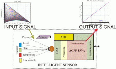
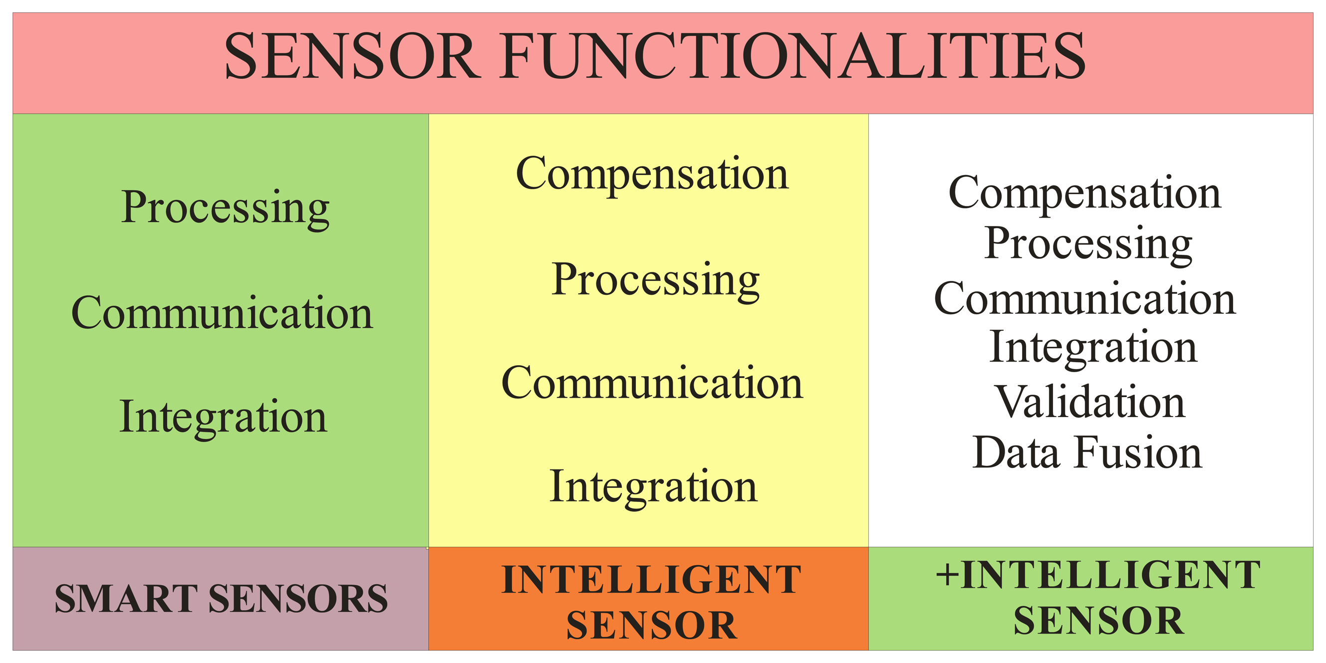
2.1. Intelligent Sensors Functionalities
2.2. Progressive Polynomial for Self-adjustment Method
- Based on the adjustment process of measuring systems [27], N readjustment points into of measurement range of the sensor are chosen and called readjustment vector, x′. The readjustment vector is supplied to the sensor and the output signal is recorded to generate the vector y′. Using Equations (2) and (3) the signals are normalized to get x(i) = [x1,x2,…,xN] and y(i) = [y1,y2,…,yN] for i = 1 to N. The ideal output for each point is defined by Equation (4), t(i) = [t1,t2,…,tN]. These values are required only to compute the coefficients k1 to kN as described in the following steps.
- With the first points x1, y1 and t1 any offset problem is fixed. This involves computing coefficient k1:and a new function f1 is defined as follows:If the y function does not include an offset error, the coefficient k1 is zero and the equation f1 is equal to y. Remember, the normalized output signal for any input signal is represented by y and this signal is generated by the sensor under normal operation.
- Using the points x2 and y2 the gain problem, if any, is eliminated. Where x2 is the upper limit of the measure scale. Then the k2 coefficient is obtained by:The new function f2(k2,t1, f1), without the gain problem is defined as:If a gain error is not observed in y, the k2 coefficient is zero and equation f2 is equal to equation f1.For sensors with linear transfer function three foregoing steps are enough to self-readjustment of the sensor, but if the transfer function is nonlinear, more coefficients k and functions f are required.
- If the transfer function of the sensor is nonlinear, a new set of coefficients and functions are defined. The coefficients k3 to kN are defined by:and the function f3 to fN defined by:The new transfer function of the sensor is represented by:
3. Improved Progressive Polynomial Algorithm to Self-Adjustment
3.1. Permutation Vector Analysis
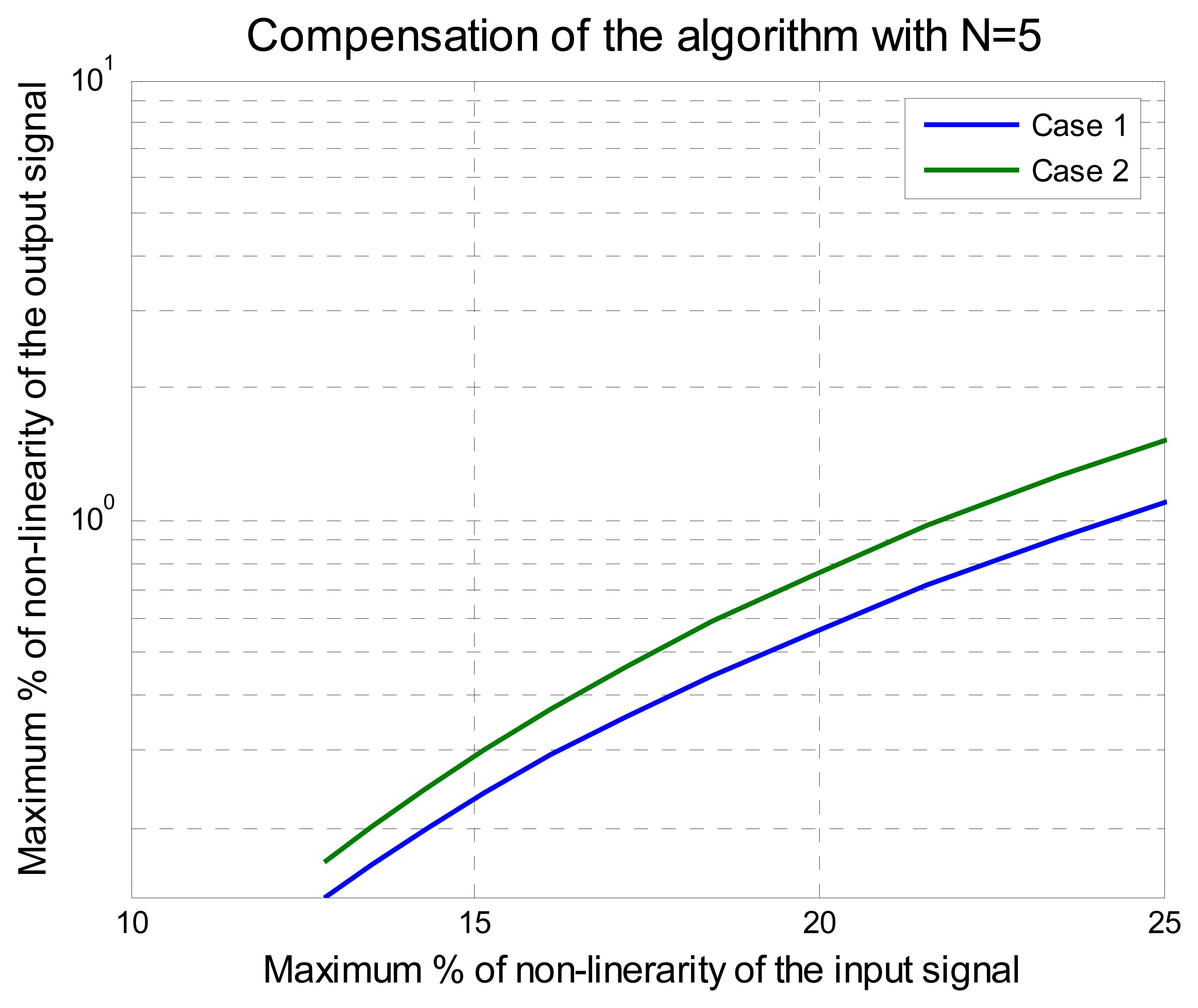
- Case 1 with:
- xN = [0, 1.0, 0.45, 0.15, 0.30], N = 5
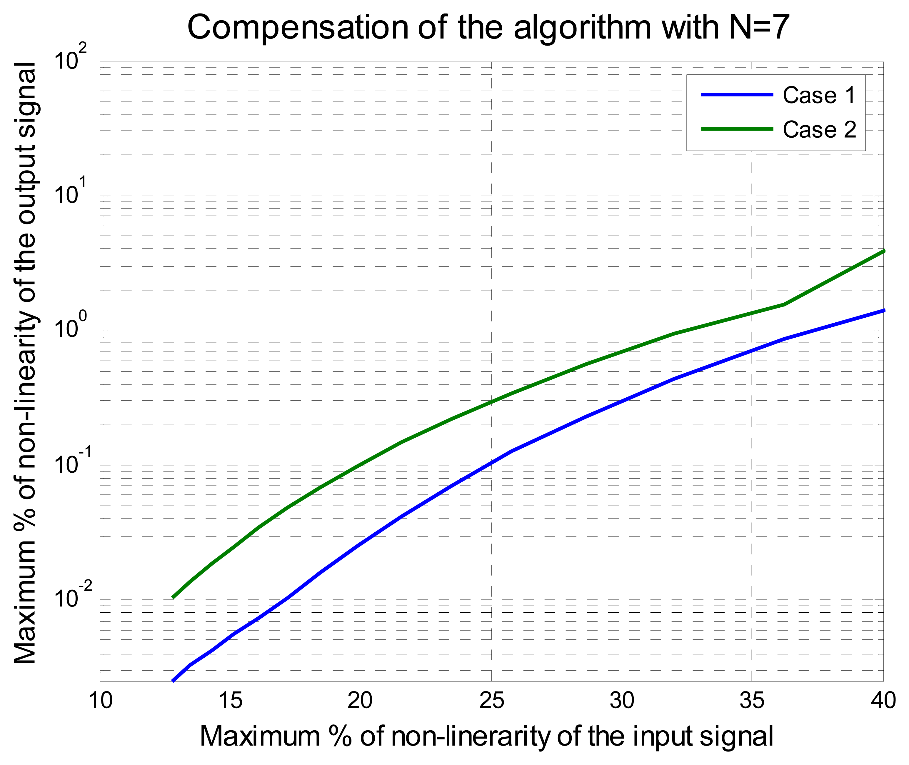
- xN = [0, 1.0, 0.45, 0.15, 0.30, 0.60, 0.75], N = 7
- and Case 2 with:
- xN = [0, 1.0, 0.15, 0.30, 0.45], N = 5
- xN = [0, 1.0, 0.15, 0.30, 0.45, 0.60, 0.75], N = 7
3.2. Improved Polynomial Progressive Algorithm with Permutation Vector Analysis
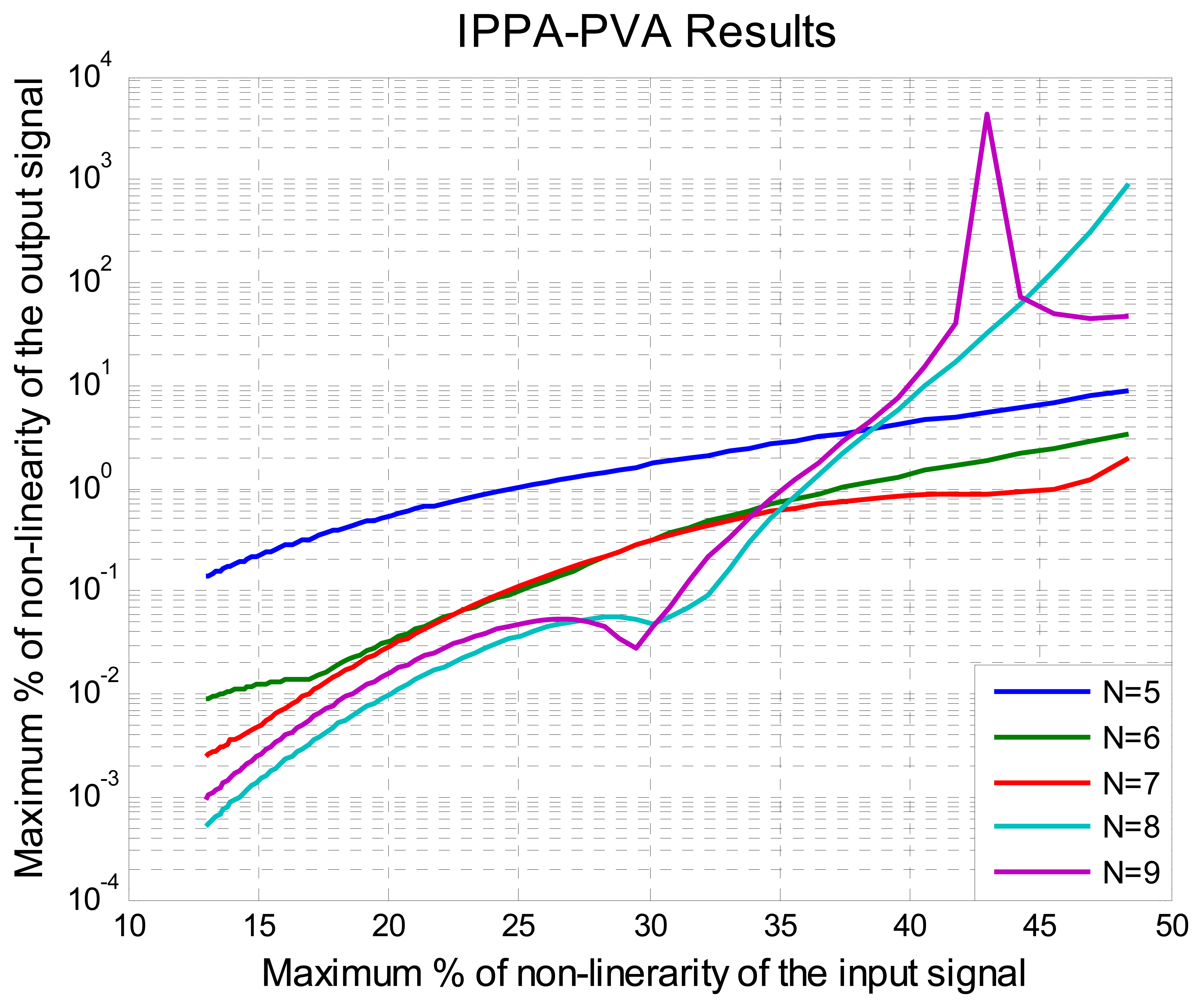
- xN = [0, 0.15, 0.30, 0.45, 1], N=5
- xN = [0, 0.15, 0.30, 0.45, 0.6, 1], N=6
- xN= [0, 0.15, 0.30, 0.45, 0.60, 0.75, 1], N=7
- xN = [0, 0.14, 0.28, 0.42, 0.56, 0.70, 0.84, 1], N=8
- xN = [0, 0.12, 0.24, 0.36, 0.48, 0.60, 0.72, 0.84, 1], N=9
- , N=5
- , N=6
- , N=7
- , N=8
- , N=9
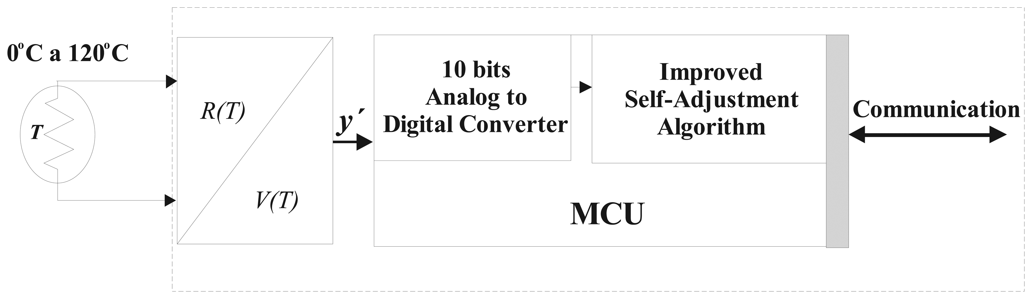
4. Intelligent Sensor Design with IPPA-PVA for self-Adjustment implemented on small MCU
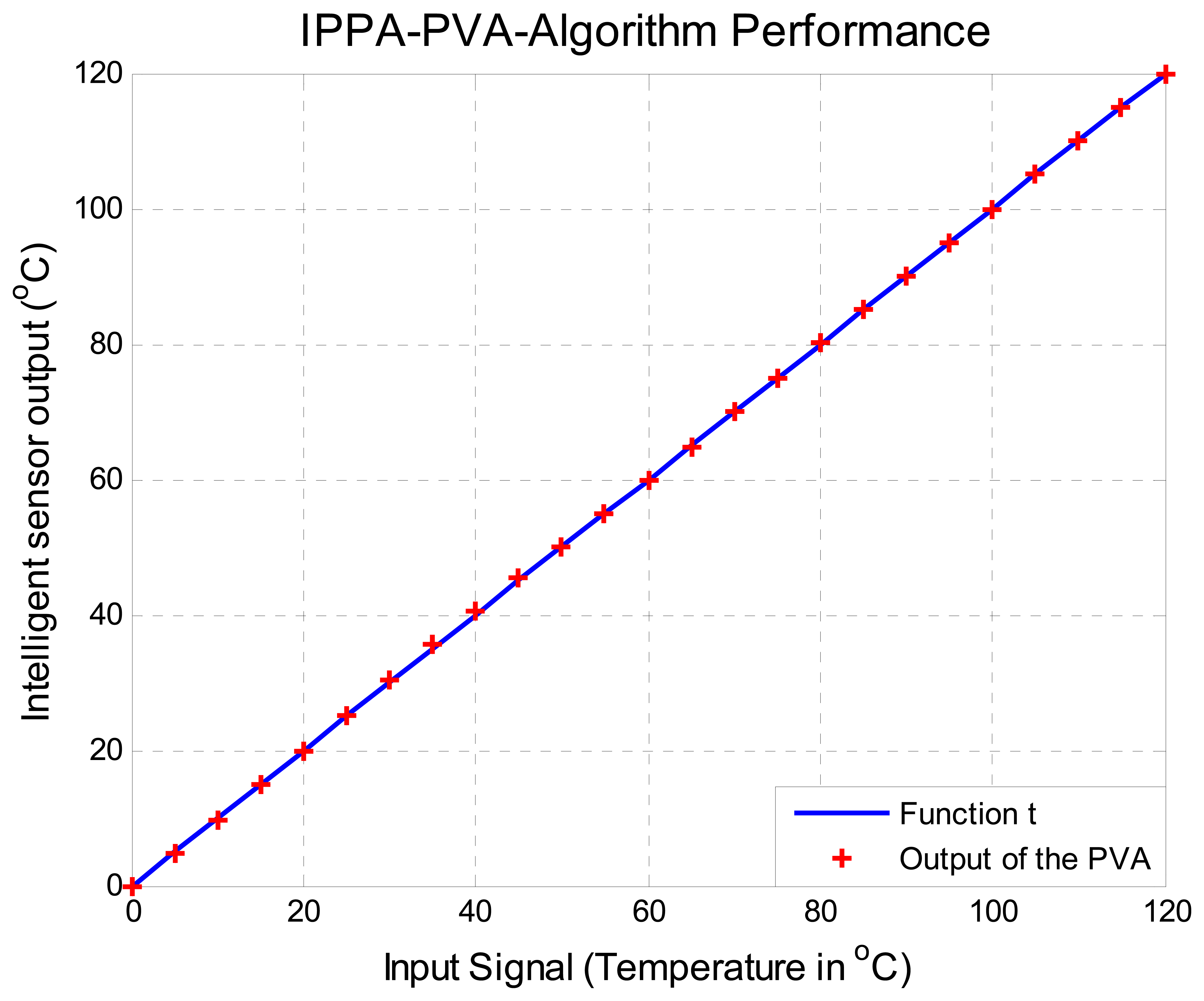
5. Tests and Results
6. Conclusions
Acknowledgments
References
- Khachab, N.I.; Ismail, M. Linearization Techniques for n-th Order Sensor Model in Mos VLSI Technology. IEEE Trans. Circuits Syst. 1991, 38, 1439–1449. [Google Scholar]
- Guangbin, Z.; Sooping, S.; Jin, L.; Sterrantino, S.; Johnson, D.K.; Jung, S. An Accurate Current Source With On-Chip Self-Calibration Circuits for Low-Voltage Current-Mode Differential Drivers. IEEE Trans. Circuits Syst. 2006, 53, 40–47. [Google Scholar]
- Iglesias, G.E.; Iglesias, E.A. Linearization of Transducer Signal Using an Analog to Digital Converter. IEEE Trans. Instrum. Meas. 1988, 37, 53–57. [Google Scholar]
- Vargha, B.; Zoltán, I. Calibration Algorithm for Current-Output R-2R Ladders. IEEE Trans. Instrum. Meas. 2001, 50, 1216–1220. [Google Scholar]
- Dent, AC.; Cowan, C. F.N. Linearization of Analog to Digital Converters. IEEE Trans. Circuits Sys. 1990, 37, 729–737. [Google Scholar]
- Kaliyugavaradan, S.; Sankaran, P.; Murti, V.G. K. A New Compensation Scheme for Thermistors and its Implementation for Response Linearization Over a wide Temperature Range. IEEE Trans. Instrum. Meas. 1993, 42, 952–956. [Google Scholar]
- Cristaldi, L.; Ferro, A.O; Lazzaroni, M.; Ottoboni, R. A Linearization Method for Commercial Hall-Effect Current Transducer. IEEE Trans. Instrum. Meas. 2001, 50, 1149–1153. [Google Scholar]
- Malcovati, P.; Leme, C.A.; O'Leary, P.; Maloberti, F.; Baltes, H. Smart sensor interface with A/D conversion and programmable calibration. IEEE J. Solid-State Circuits 1994, 29, 963–966. [Google Scholar]
- Yamada, M.; Watanabe, K. A capacitive pressure sensor interface using oversampling Δ-Σdemodulation techniques. IEEE Trans. Instrum. Meas. 1997, 46, 3–7. [Google Scholar]
- Taylor, J.H.; Antoniotti, A.J. Lineariation Algorithm for Computer Aided Control Engineering. IEEE Control Syst. Mag. 1993, 58–64l. [Google Scholar]
- Patranbis, D.; Gosh, D. Anovell software based transducer linearizer. IEEE Trans. Instrum. Meas. 1989, 38, 1122–1126. [Google Scholar]
- Kikuchi, S.; Tsuji, H.; Sano, A. Autocalibration Algorithm for Robust Capon Beamforming. IEEE Antennas Wirel. Propag. Lett. 2006, 5, 251–255. [Google Scholar]
- Depari, A.; Flammini, A.; Marioli, D.; Taroni, A. Application of an ANFIS Algorithm to Sensor Data Processing. IEEE Trans. Instrum. Meas. 2007, 56, 75–79. [Google Scholar]
- Depari, A.; Ferrari, P.; Ferrari, V.; Flammini, A.; Ghisla, A.; Marioli, D.; Taroni, A. Digital Signal Processing for Biaxial Position Measurement With a Pyroelectric Sensor Array. IEEE Trans. Instrum. Meas. 2006, 55, 501–506. [Google Scholar]
- Hooshmand, R.A.; Joorabian, M. Design and optimisation of electromagnetic flowmeter for conductive liquids and its calibration based on neural networks. IEE Proc. Sci. Meas. Technol. 2006, 153, 139–146. [Google Scholar]
- Abu, K.N.; Lonsmann, I.J.J. Calibration of a Sensor Array (an Electronic Tongue) for Identification and Quantification of Odorants from Livestock Buildings. Sensors 2007, 7, 103–128. [Google Scholar]
- Patra, J.C.; Luang, A.E.; Meher, P.K. A Novel Neural Network-based Linearization and Auto-compensation Technique for Sensors. Presented at the IEEE International Symposium on Circuits and Systems, Island of Kos, Greece, May 2006.
- Tao, J.; Qingle, P.; Xinyun, L. An Intelligent Pressure Sensor Using Rough Set Neural Networks. Proceedings of the IEEE International Conference on Information Acquisition, Shandong, China, July 2006.
- Hutchins, M.A. Twenty-First Century Calibration; The Institution of Electrical Engineers the IEE, 1996; Savoy Place, London WC2R OBL, UK. [Google Scholar]
- Dack, P. So What Does Industry Want From Calibration. IEE Colloquium on The Contribution of Instrument Calibration to Product Quality, London, UK, 25 Apr 1995; pp. 2/1–2/6.
- Williams, T.A. Quality Management: Quality Spending Nears $3B Mark. Qual. Mag. Improving Manuf. Process. 2004. www.qualitymag.com August 2006.
- Robins, M. Quality Management: $4.4 Billon and Growing. Qual. Mag. Improving Manuf. Process. 2005. www.qualitymag.com.
- Powell, G. Calibration Services to Continue Growth Path. Qual. Mag. Improving Manuf. Process. 2003. www.qualitymag.com.
- Rivera, M.J.; Carrillo, R.M.; Chacón, M.M.; Herrera, R.G.; Bojoquez, G. Self-Calibration and Optimal Response in Intelligent Sensors Design Based on Artificial Neural Networks. Sensors 2007, 7, 1509–1529. [Google Scholar]
- Fouad, L.K.; Horn, G.; Huijsing, J.H. A Noniterative Polynomial 2-D Calibration Method Implemented in a Microcontroller. IEEE Trans. Instrum. Meas. 1997, 46, 752–757. [Google Scholar]
- Dias, P.J.M.; Postolache, O.; Silva, G.P. Adaptive Self-Calibration Algorithm for Smart Sensors Linerization. Presented at the IEEE Instrumentation and Measurement Technology Conference, Ottawa, Ontario, Canada, May 2005.
- ISO International vocabulary of basic and general terms in metrology, 2nd Edition ed; ISO Publishing: Geneve, Switzerland, 1993.
- Hernandez, W. Improving the Response of a Rollover Sensor Placed in a Car under Performance Tests by Using a RLS Lattice Algorithm. Sensors 2005, 5, 613–632. [Google Scholar]
- Frank, R. Understanding Smart Sensors; Artech House: Norwood, Massachusetts, 2000. [Google Scholar]
- Samir, M. Further Structural Intelligence for Sensors Cluster Technology in Manufacturing. Sensors 2006, 6, 557–577. [Google Scholar]
- Hernandez, W. Improving the Response of a Load Cell by Using Optimal Filtering. Sensors 2006, 6, 697–711. [Google Scholar]
- Miskowiccz, M. Asimptotic Effectiveness of the Event-Based Sampling according to the Integral Criterion. Sensors 2007, 7, 16–37. [Google Scholar]
- Hernandez, W. A Survey on Optimal Signal Processing Thechniques Applied to Improve the Performance of Mechanical Sensors in Automotive Applications. Sensors 2007, 7, 84–102. [Google Scholar]


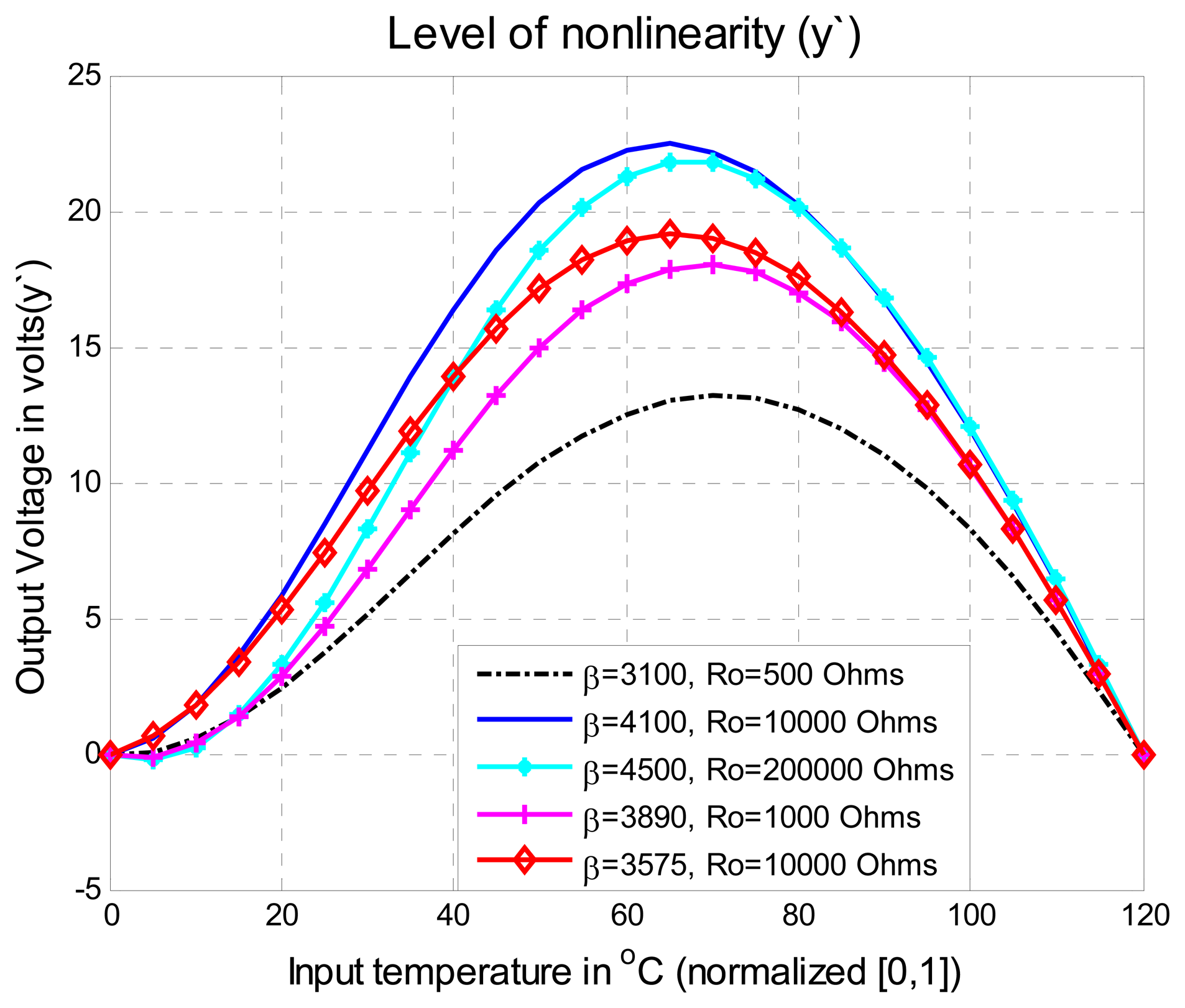
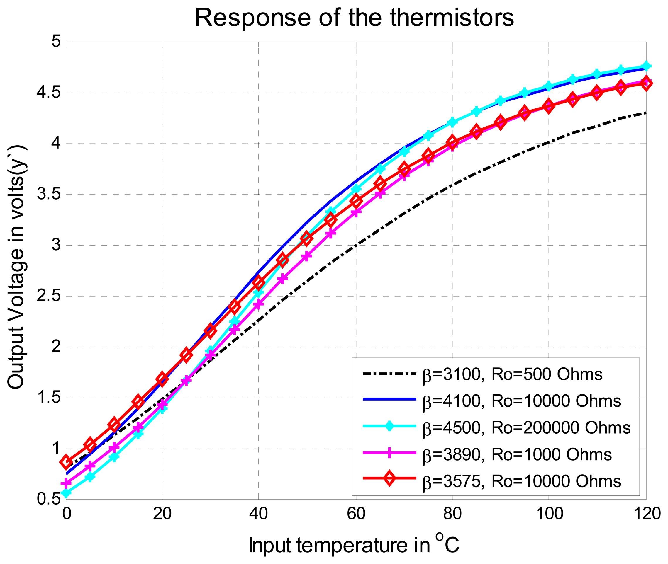
| Thermistors Features | % max. initial error εr | Order of the vector | % max εr6 of |
|---|---|---|---|
| β=3100; To=25°C Ro=500 Ohms | 13.20% | -0.043 a 0.0192 | |
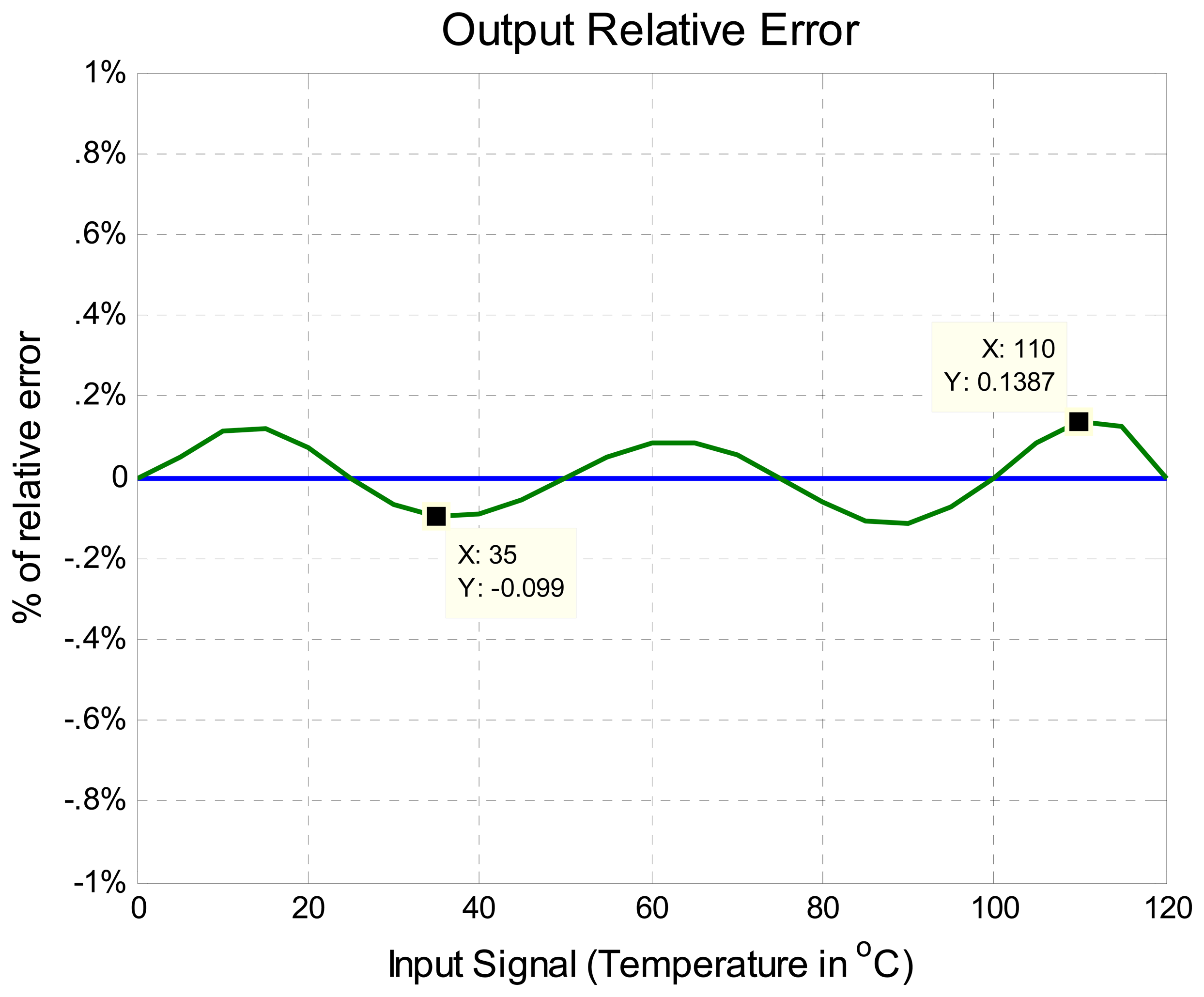
| β=4100; To=25°C Ro=10000 Ohms | 22.47% | -0.099 a 0.1383 | |
| β =4500; To=25 Ro=200000 Ohms | 21.79% | -0.155 a 0.1931 | |
| β =3890; To=25°C Ro=1000 Ohms | 18.02% | -0.099 a 0.091 | |
| β =3575; To=25°C Ro=10000 Ohms | 19.17% | -0.0493 a 0.0718 | |
© 2008 by the authors; licensee Molecular Diversity Preservation International, Basel, Switzerland. This article is an open-access article distributed under the terms and conditions of the Creative Commons Attribution license (http://creativecommons.org/licenses/by/3.0/).
Share and Cite
Rivera, J.; Herrera, G.; Chacón, M.; Acosta, P.; Carrillo, M. Improved Progressive Polynomial Algorithm for Self-Adjustment and Optimal Response in Intelligent Sensors. Sensors 2008, 8, 7410-7427. https://doi.org/10.3390/s8117410
Rivera J, Herrera G, Chacón M, Acosta P, Carrillo M. Improved Progressive Polynomial Algorithm for Self-Adjustment and Optimal Response in Intelligent Sensors. Sensors. 2008; 8(11):7410-7427. https://doi.org/10.3390/s8117410
Chicago/Turabian StyleRivera, José, Gilberto Herrera, Mario Chacón, Pedro Acosta, and Mariano Carrillo. 2008. "Improved Progressive Polynomial Algorithm for Self-Adjustment and Optimal Response in Intelligent Sensors" Sensors 8, no. 11: 7410-7427. https://doi.org/10.3390/s8117410