Laboratory Evaluation of Acoustic Backscatter and LISST Methods for Measurements of Suspended Sediments

Abstract

The limitation of traditional sampling method to provide detailed spatial and temporal profiles of suspended sediment concentration has led to an interest in alternative devices and methods based on scattering of underwater sound and light. In the present work, acoustic backscatter and LISST (the Laser In Situ Scattering Transmissometry) devices, and methodologies were given. Besides a laboratory study was conducted to compare pumping methods for different sediment radiuses at the same concentration. The glass spheres (ballotini) of three different radiuses of 115, 137 and 163 μm were used to obtain suspension in the sediment tower at laboratory. A quite good agreement was obtained between these methods and pumping results with the range at 60.6-94.2% for sediment concentration and 91.3-100% for radius measurements. These results and the other studies show that these methods have potential for research tools for sediment studies. In addition further studies are needed to determine the ability of these methods for sediment measurement under different water and sediment material conditions.

1. Introduction

The transport of suspended sediments has a growing interest because of environmental pollution, siltation problem in water storage structures and channels, and the removing of fine soil from agricultural lands. Measuring suspended sediment is difficult as it changes temporally and spatially with the effects of flow and turbulence.

The traditional sediment measurement method is to take periodic water samples for water analyses. Application of this method is simple, but labor intensive to collect and process. Also, this method is restrictive in its capability to provide detailed spatial and temporal profiles of suspended sediment concentration. Over the past decade, technological advances in electronics and computer sciences have led to new devices that produce accurate measurements of suspended sediment concentration in water. In particular, instruments based on the scattering of underwater sound [1-4], and light [5-7], have been investigated in some detail for suspended sediment measurements.

The acoustic backscatter system (ABS) involves the propagation of sound around a megahertz through the water column. Short bursts of high frequency sound, 0.5 MHz -5.0 MHz, those transmitted from a transducer are directed towards the measurement volume. Sediment in suspension directs a portion of this sound back to the transducer. The strength of the backscattered signal allows the calculation of sediment concentration. The backscatter amplitude depends on the concentration, particle size, and acoustic frequency. This can be exploited by using multiple frequencies to determine both particle size and concentration. The strong signal from the bed can be used to measure the bed forms. Acoustic devices measure the concentration in a range-gated vertical profile of 1-2 m in depth [8-10].

This method has been demonstrated and utilised successfully under laboratory and field conditions by several investigators. Results showed that sediment concentration and particle size can be measured relatively non-intrusive, with high spatial and temporal resolution with acoustic backscatter systems. But acoustic measurement has some limitations; the signal is susceptible to absorption and scattering by bubbles, from the biological materials and flow depth limitation for shallow rivers [11].

In recent years, the application of laser scattering techniques have opened new possibilities for the measurement of sediment concentration and size distribution. The LISST-100 (the Laser In Situ Scattering Transmissometry) which is developed by Sequoia Scientific Inc. for laser scattering technique, directs a laser beam through a sample of water where particles in suspension will scatter, absorb and reflect the beam. The diffracted laser beam is received by ring detectors that allow measurement of the scattering angle of the beam. Particle size and volumetric concentration can be calculated from knowledge of this angle [12, 13]. Gartner et al., (2001) have reported that laboratory and field measurements indicate the potential of the LISST as a powerful research tool for sediment measurement studies and the instrument is capable of determining size distribution and volume concentration within acceptable limits [7]. Traykovski et al. (1999) performed several experiments with natural sediments in the laboratory to compare LISST results to traditional sieving, filtering and weighing techniques [14]. They found the LISST was able to adequately determine the particle volumetric size distribution of two different natural sediments. Van Wijgaarden and Roberti (2002) have used LISST for the measurement of the particle size and settling velocity of suspended sediment in calm fresh water [15] and Thonon et al. (2005) have used LISST on river floodplains [16]. Both of these authors report a greatly expanded capacity for the collection of the spatial and temporal variability of suspended sediment in these conditions.

A disadvantage of the LISST instrument is its large size, which causes a significant flow obstruction. Another disadvantage is the design of the LISST laser mount, which is sensitive to impacts that can easily throw it out of alignment. The high energy regime of the surf zone could easily provide impacts of such magnitude [11].

These methods are still in an ongoing developmental phase and the studies are needed to introduce and explore of methodology details and to compare with each other. The objectives of this paper are to describe of ABS and LISST devices, to give an explanation of the basic physics which is used to interpret the backscatter signal methodology, and to determine methods of mean mass concentration and mean particle size using LISST results of volumetric particle size distribution. Finally a laboratory study was conducted to compare ABS and LISST methods with pumping method for different sediment radius.

1.1 Acoustic methodology; backscattering

The concentration of suspended sediments in water can be determined from backscattered signal from suspensions using following approach [17, 18, 10, 9, 2, 19, 1]. The suspended sediment concentration M, can be expressed as:

$$M={\left\{\frac{V_{\mathit{\text{rms}}}\psi r}{k_S{k}_t}\right\}}^2{e}^{4r({\alpha }_w+{\alpha }_s)}$$

(1)

M is the suspended sediment concentration, V_rms is recorded voltage from the transducer, ψ, accounts for the departure from spherical spreading within the transducer nearfield.

$$\psi =\frac{1+1.35z+{(2.5z)}^{3.2}}{1.35z+{(2.5z)}^{3.2}}$$

(2)

where;

$$z=r/rn,r_n=\pi {a_t}^2/\lambda$$

a_t is the effective radiating radius of the transducer, λ is the sound wavelength and r is range from transducer. k_t is a constant and found from calibration, α_w is the attenuation coefficient due to water absorption; its dependence upon water temperature, depth and salinity can be obtained from tables or by formulae. The absorption of sound for freshwater at atmospheric pressure can be written as [20]:

$${\alpha }_w=(55.9-2.37T+4.77*{10}^{-2}{T}^2-3.84*{10}^{-4}{T}^3){10}^{-3}f{r}^2$$

(3)

T is degrees Celsius, f_r frequency in MHz. α_s is the attenuation due to scattering in suspension and can be described by

$${\alpha }_S=\frac{1}{r}\int \xi (r)M(r)$$

(4)

$$\xi =\frac{3}{4a_S\rho }\chi$$

(5)

χ, is the normalised total scattering cross-section. a_s is the radius of the particles in suspension. ρ_S is the density of the particles in suspension (∼2650 kg.m^-3 for sandy sediments).

$$k_S=\frac{f}{\sqrt{a_S{\rho }_S}}$$

(6)

f is form function and describes scattering properties of the particle. The normalised total scattering cross-section and form function values are related with particle radius and wave number of the sound(k) in water. This relation was given by Thorne and Meral (2008) as [21];

$$\chi =\frac{0.29{({\mathit{\text{ka}}}_S)}^4}{0.95+1.28{({\mathit{\text{ka}}}_S)}^2+0.25{({\mathit{\text{ka}}}_S)}^4}$$

(7)

$$f=\frac{{\mathit{(}{\mathit{\text{ka}}}_S\mathit{)}}^2\mathit{(}1-0.35e^{-{\mathit{(}\mathit{(}{\mathit{\text{ka}}}_S-1.5\mathit{)}/0.7\mathit{)}}^2}\mathit{)}\mathit{(}1+0.5e^{-{\mathit{(}\mathit{(}{\mathit{\text{ka}}}_S-1.8\mathit{)}/2.2\mathit{)}}^2}\mathit{)}}{1+0.9{\mathit{(}{\mathit{\text{ka}}}_S\mathit{)}}^2}$$

(8)

Calibration constant, k_t, is determined from the acoustic backscatter strength of homogenous suspended sediment of known particle size and concentration level.

Suspended sediment equation (Eq. (9)) contains two M values. If the all other equation parameters are known the following procedures are used for obtaining suspended sediment concentration and particle size.

$$M={\left\{\frac{V_{\mathit{\text{rms}}}\psi r}{k_s{k}_t}\right\}}^2{e}^{4r\left[\frac{1}{r}\int \xi (r)M(r)\right]}$$

(9)

The second M (on right of equation) is accepted as zero and the first M is computed which is called M₀. After that the final M value is computed using M₀ with Eq.(9). This procedure is applied for different particle radiuses and each range(r) values, and β coefficients are computed for selected particle radius.

$$\beta =\frac{M_{\mathit{\text{std}}}}{M_{\mathit{\text{mean}}}}$$

(10)

where; M_std is standard deviation and M_mean is mean of computed M values. The particle radius is chosen as real one which gives a minimum β value [1].

1.2 The LISST-100 devices and principle of laser scattering; diffraction

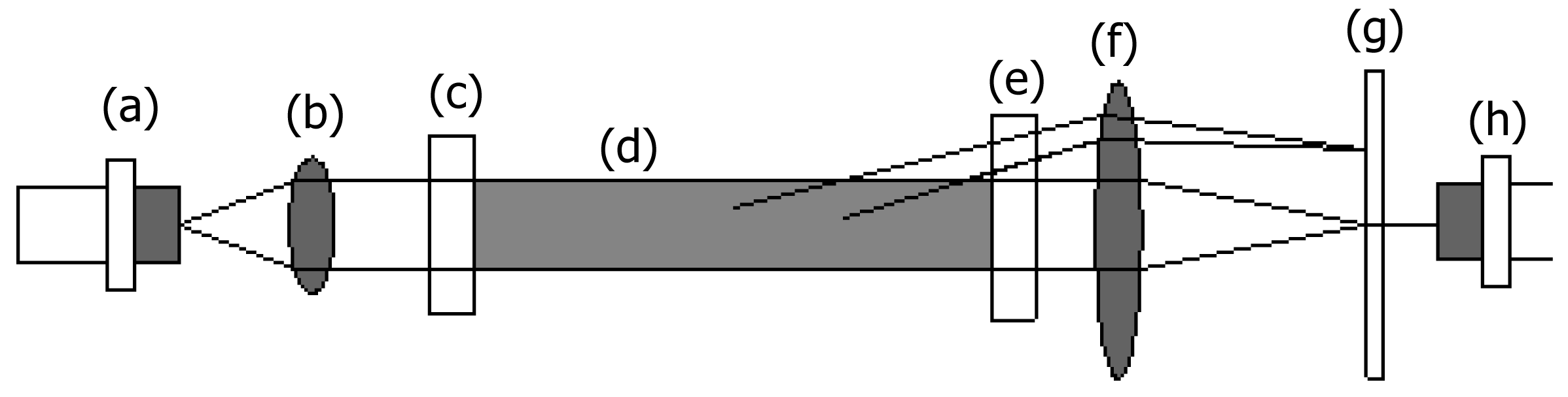
The LISST-100, with diameter of 13 cm and length of 81 cm, is a laser particle size analyser and consists of a diode laser operating at 670 μm which is collimated to form a parallel beam of light (figure 1). The beam passes through a 5 cm sample cell of water where particles produce scattering. The forward diffracted beam is collected by a set of 32 ring detectors that are logarithmically spaced and located in the focal plane of the laser receiving lens. Each ring detector measures scattering over a sub-range of angles. The ring radius and focal plane length of the receiving lens determine the range of the angles. A photo-diode is placed behind the ring detector which detects the main laser beam. This supplies the optical transmissometer function [5].

The light scattering measured by the LISST represents light scattering within a thin radial annulus in the focal plane of radius r and with dr. This annulus represents an area, dA=2 πrdr, and the light gathered by this annulus is all the light that is forward scattered into the solid range for distance f is, θ+dθ =atan(r+dr/f). The scattering per unit solid angle into angle θ, from a single particle radius is defined as light power(energy). The light power can be written in the matrix form (K_i,j) for each detector (i= 1, 2, 3……N) and each size class (j =1, 2, 3……N), and its relation between the volume distribution (Vj) can be expressed as;

$$E_i=K_{i,j}{V}_j$$

(11)

$$V_j=\underset{a_{j,min}}{\overset{a_{j,max}}{\int }}{a}^{3}n(a)\mathit{\text{da}}$$

(12)

a_j,min and a_j,max are minimum and maximum particle diameter in the jth class and n(a) is the number of particles of size [13].

The scattered power must be corrected with background scattering, z, the optical transmission, τ, which is recorded by optical transmissometer, and detector correction factor (D_c) which is provided by the instrument manufacturer.

$$E=D_c\lfloor \left(E_i/\tau \right)-z\rfloor$$

(13)

The background scattering is recorded to account for the optical effect of the flow-through chamber. To obtain z, the flow-through chamber is filled with clear water, and LISST scans are recorded and averaged.

Finally, the volume concentration;

$$V=\frac{D_c\lfloor \left(E_i/\tau \right)-z\rfloor }{Cv}$$

(14)

C_v, volume conversion constant, is determined from LISST measurement of known volume concentration particles (V₀). The background scattering distribution from de-ionised water, and the scattering distribution from the suspension are recorded, and E is computed. Finally volume conversion constant,

$$C_v=\sum E/V_0$$

(15)

LISST measurements were logged using a standard LISST-TOP software provided by Sequoia Scientific and further processed in the MATLAB.

2. Materials and Methods

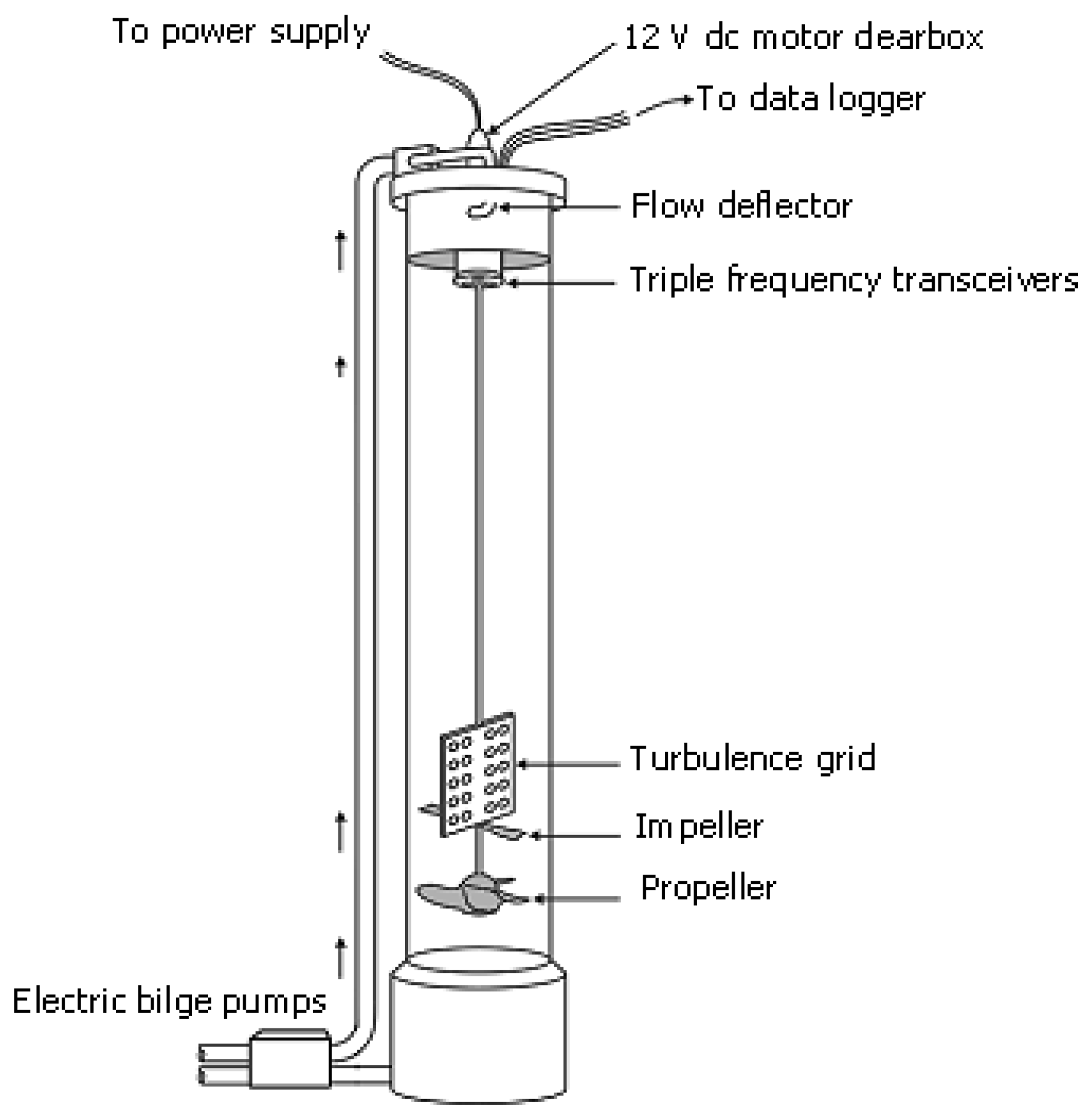
This experiment was carried out under laboratory conditions and all measurements were conducted in the vertical sediment tower shown in figure 2. The tower was built to obtain a homogeneous suspension of sediments within the central region of the tower, using the re-circulation bilge pumps and a mixing unit composed of a turbulence grid impellor and propeller driven by a 12 V dc motor. The ABS transducers are located around the central shaft of the grid shaft [22].

Initially the tower was filled with water and the system was run to remove bubbles in the water for fifteen minutes every fifteen minutes during 3 days which is known as degassing. The ABS background measurements were taken during one hour using 3 different transducers operating at 1, 2 and 4 MHz frequencies.

Before starting of LISST measurement, the background scattering distribution was measured using clear water to take into scattering and attenuation due to water itself.

The glass spheres (ballotini) of three different radiuses of 115, 137 and 163 μm with a 10% variation in the mean size, were used to prepare of suspended sediment because all the acoustic parameters were known and they provided an unambiguous condition of the prediction of sediment concentration. 120 gr wetted and degassed ballotini was added to the tower for each radius application and homogeneous suspension was obtained with the circulation of water with pump and mixer unit which consist of turbulence grid, impeller and propeller. ABS and LISST measurements were taken during 1 hour for each radius, and pumping samples were taken three times during this period. The average suspended sediment concentration was determined with gravimetric methods from these samples. The sediment was removed from the tower using a conical mesh, of aperture size 20 μm, placed on the top of the tower, for another experiment.

The voltage values are calculated for background (V_b) and suspended measurement (V_s) and finally backscatter voltages are obtained using the final expression;

$$V=\sqrt{{V_s}^2-{V_b}^2}$$

(16)

LISST-100 Particle Size Analyzer program gives results as particle size distribution and cumulative volumetric concentration for each radius. In addition a script was written to obtain mass sediment concentration, and mean particle size as follows. The LISST takes measurement for each second and each radius classes. The individual mass concentrations for each radius, M_cind, (kg.m^-3);

• $$M_{c_{\mathit{\text{ind}}}}=\rho V_c$$

  (17)

  • ρ : particle density (2480 kg.m^-3), V_c: volumetric concentration
  • The total mass concentration;
• $$M_{c_{\mathit{\text{total}}}}=\rho \sum _1^n{V}_c$$

  (18)

  • n; radius range number (1-32)
  • The mean individual mass concentrations(M_{cmean_ind}) for each radius class were obtained with considering all measurements;
• $$M_{c_{\mathit{\text{mean}}\_\mathit{\text{ind}}}}=\sum _1^m{M}_{c_{\mathit{\text{ind}}}}/m$$

  (19)

  • m; record range number

The mean sediment radius (d50) value is equal to radius versus %50 cumulative mass value

$$\%\mathit{\text{cumulative}}\_\mathit{\text{mass}}=\frac{\text{∑}_1^n{M}_{c_{\mathit{\text{mean}}\_\mathit{\text{ind}}}}}{M_{c_{\mathit{\text{total}}}}}$$

(20)

3. Results and Discussion

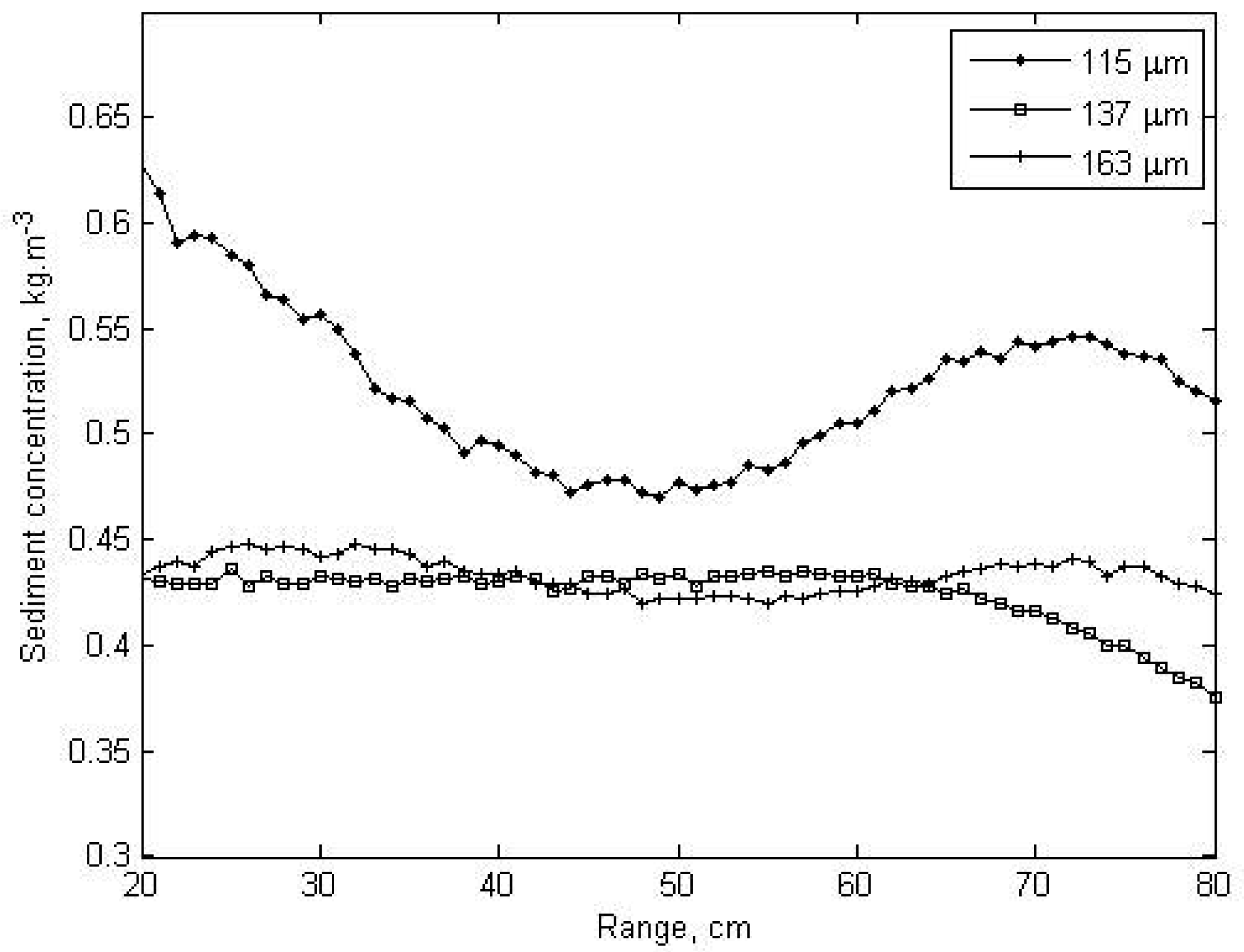
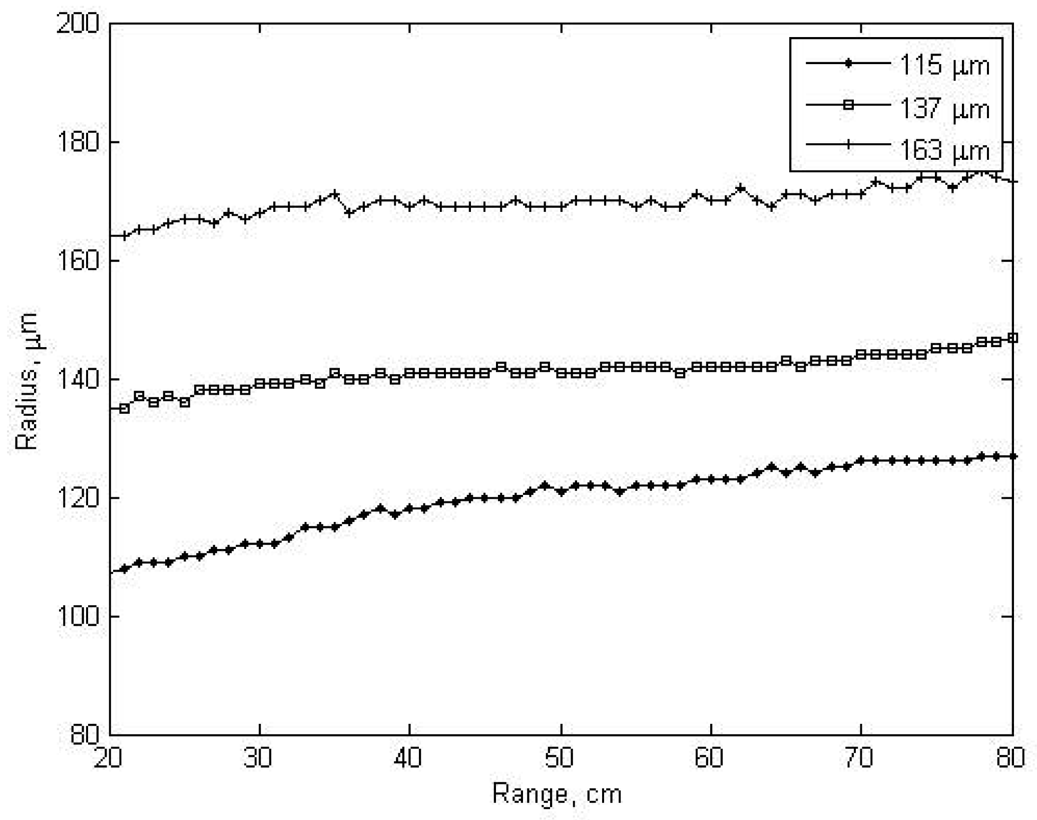
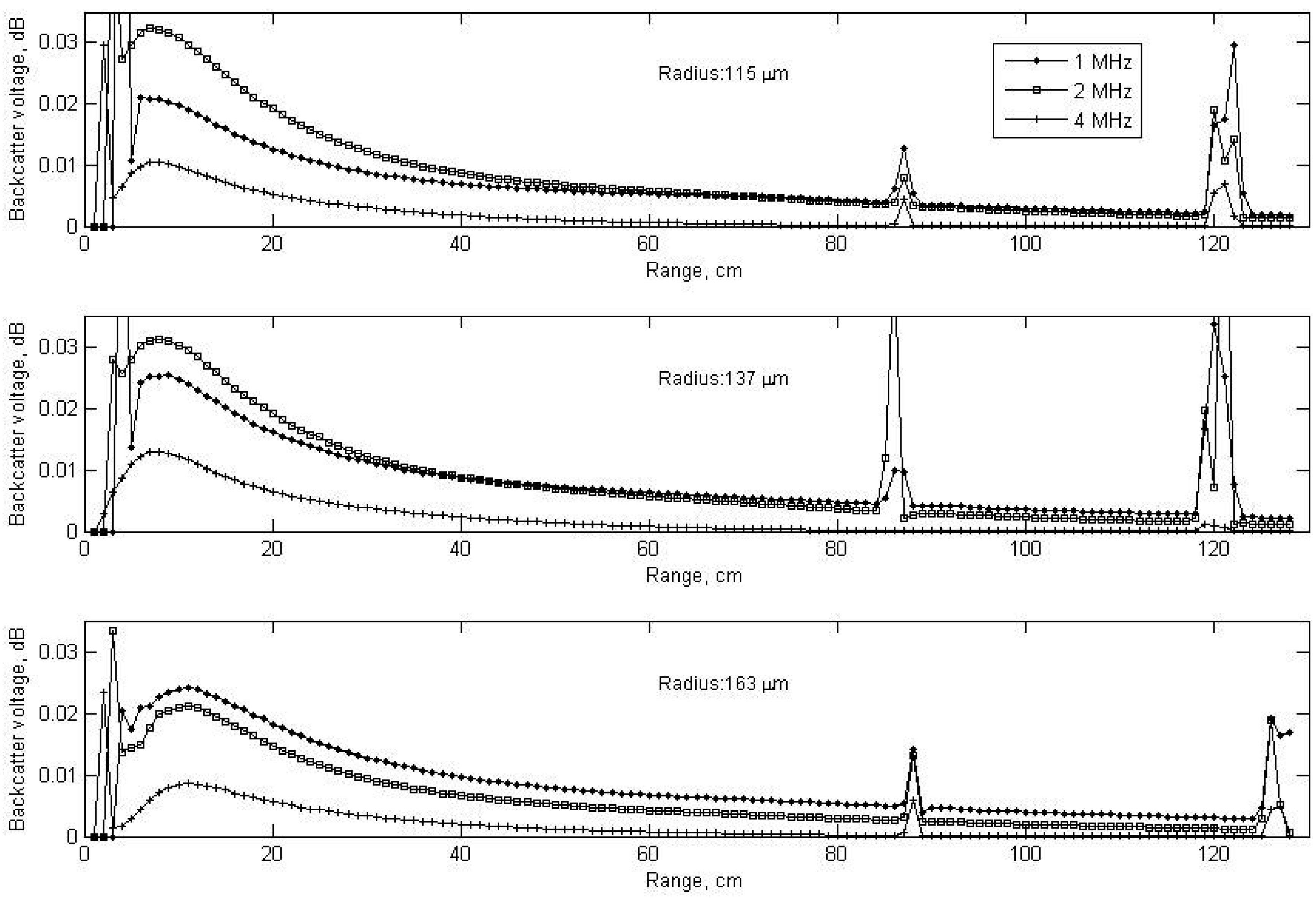
The backscatter voltage values, sediment concentration and radius results for each measurement of ABS are shown figures 3, 4 and 5. The backscatter voltages drop with increasing range from transducer. Similar results are given by Thorne at all (1991) [23] and are explained with water and particle attenuation and spreading of the beam. The nearfield region of the transducer was seen in the first 0.2 m range, and the reflections from the paddle were seen at about 0.9 m and 1.25 m. Therefore, sediment concentrations and radius were determined for 0.2-0.8 m range.

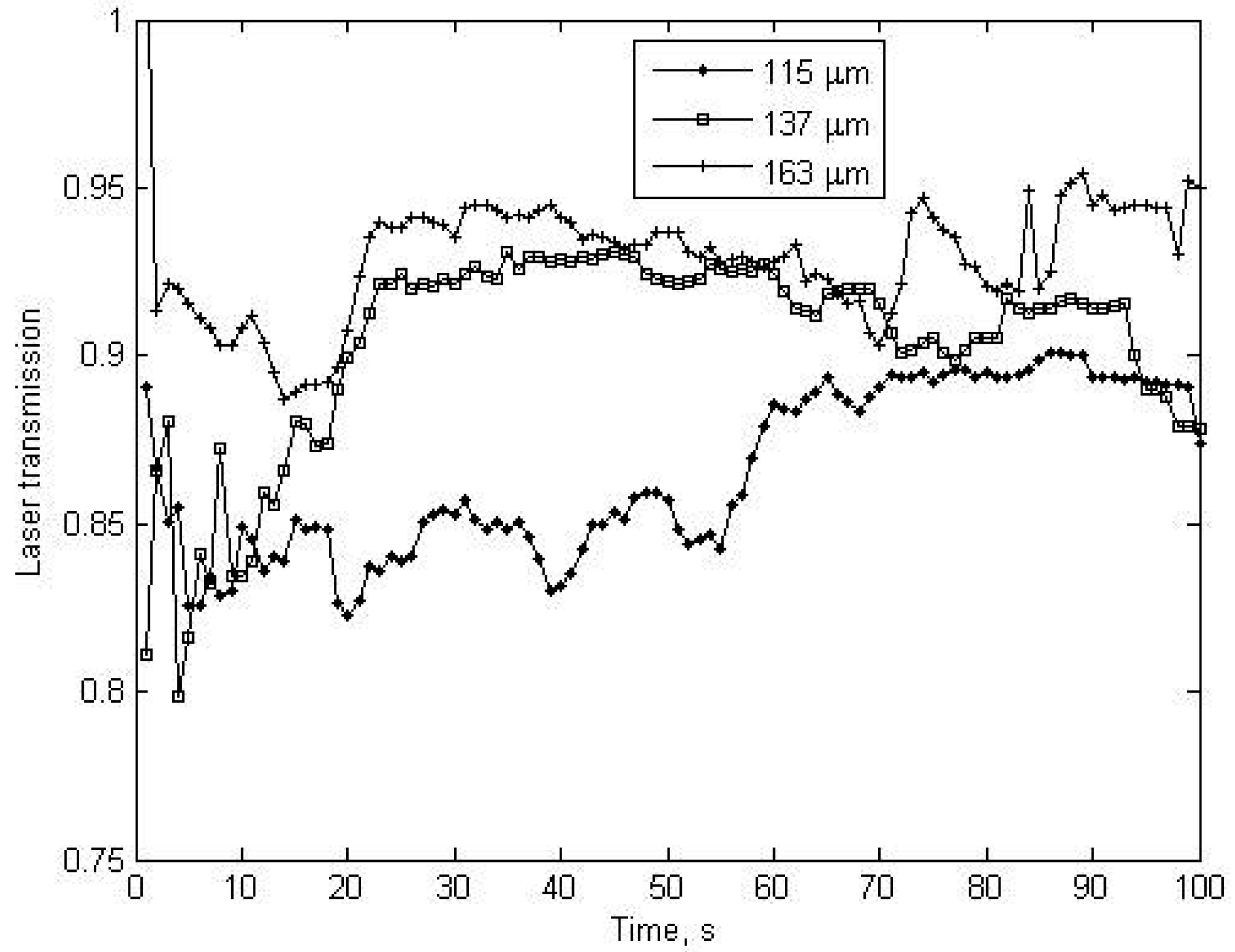
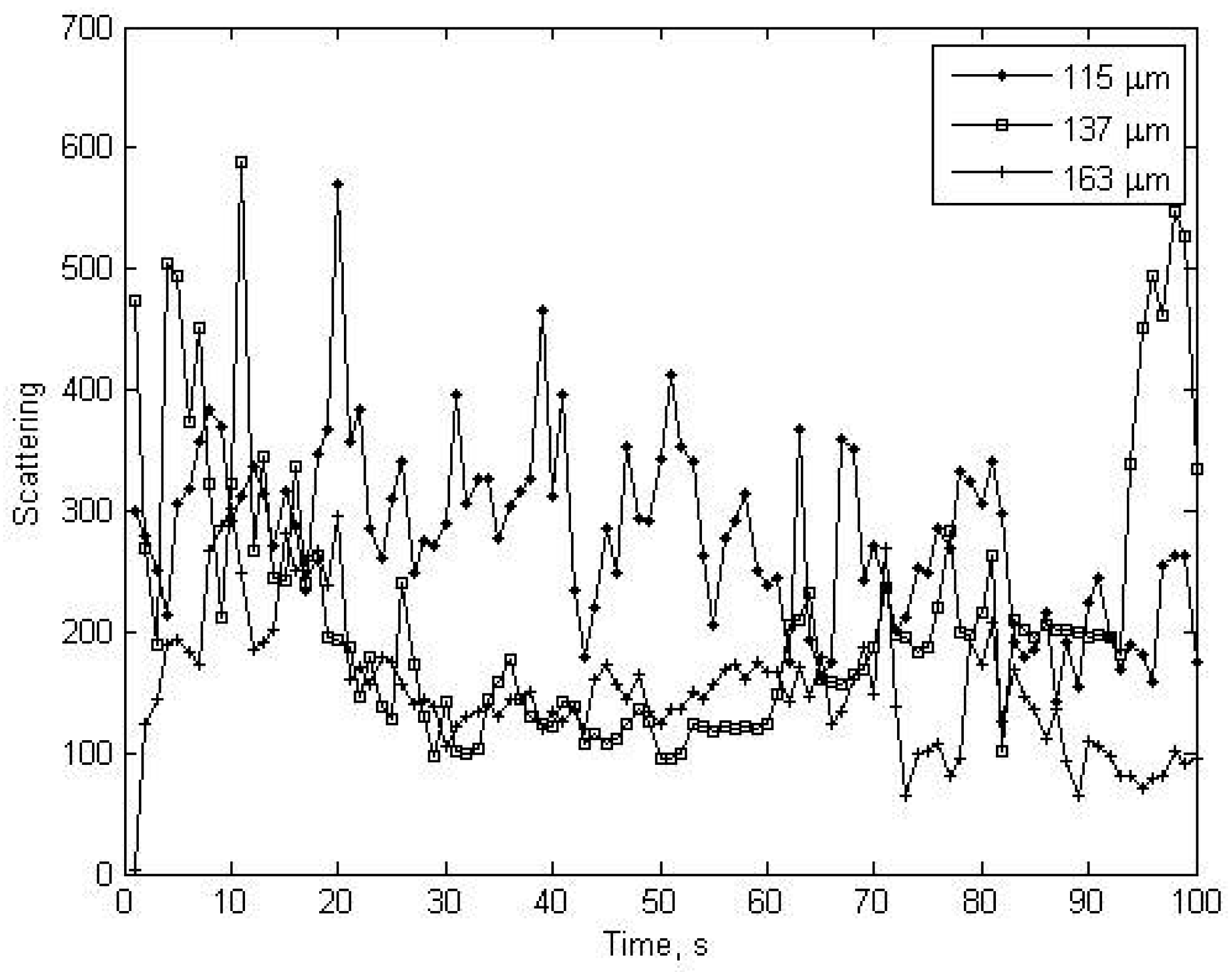
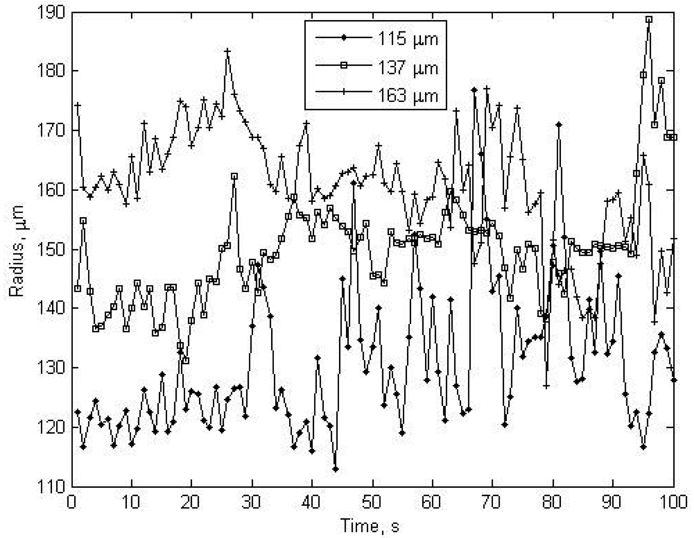
The first 100 seconds were considered because sediment concentration decreased in the course of time due to settling of ballotini. The homogenised suspension condition was obtained exactly during this time. Because when the LISST devices was put in the tower the mixing unit was stopped due to physical limitation and re-circulation was obtained just by pumps. The laser transmission, scattering distribution, sediment concentration and radius results are given each measurement of LISST in figures 6, 7, 8 and 9. Figure 6 and 8 show that the high laser transmission represents low sediment concentration, and the inverse relation is seen between radius and scattering (Figure 6 and 9).

The statistical analyses of results are tabulated in

Table 1. Sediment concentration results and statistical evaluation.

			mean	standard error	agreement with pumping,%
First measurement (115 μm)	ABS	1 MHz	0.497	0.017	90.2
		2 Mhz	0.481	0.015	87.3
		4 MHz	0.385	0.021	69.9
	LISST		0.660	0.016	80.2
Second measurement (137 μm)	ABS	1 Mhz	0.508	0.011	92.2
		2 Mhz	0.494	0.011	89.7
		4 MHz	0.275	0.011	49.9
	LISST		0.510	0.020	92.6
Third measurement (163 μm)	ABS	1 Mhz	0.519	0.012	94.2
		2 Mhz	0.486	0.009	88.2
		4 MHz	0.291	0.008	52.8
	LISST		0.334	0.012	60.6
Pumping			0.551	0.014

and

Table 2. Sediment radius results and statistical evaluation.

		mean	standard error	agreement with pumping,%
First measurement (115 μm)	ABS	110	1.314	95.6
	LISST	125	0.808	91.3
Second measurement (137 μm)	ABS	132	1.176	96.4
	LISST	131	1.237	95.6
Third measurement (163 μm)	ABS	163	1.296	100.0
	LISST	161	0.993	98.8

. ABS measurements were considered for 45 cm range and 100 s duration to compare LISST measurements under similar conditions.

Both methods have good agreement with pumping results in determining of radius. Similarly, Thosteson and Hanes (1998) found less than 20% error in laboratory test in determining sediment concentration and size [24].

In concentration measurements, the best agreement was obtained in ABS measurements for 1 and 2 MHZ frequency. Generally, 4 MHZ frequency measurements estimated lower values than the observed values and it had low agreement with pumping. This may be due to the length of transducer connection cable. It is known that signal attenuation occurs in high frequency depending upon cable length [25].

The lowest agreement (60.6%) was obtained in LISST concentration measurements for 163 μm radius. It was observed that LISST measurements were more sensitive to sediment radius. It can be said that accuracy decreases as sediment radius increases. Because LISST makes estimation based on sediment radius and radius-based scattering angle.

4. Conclusion

In both methods (ABS and LISST), quite good results were obtained for measurement of sediment concentration and radius in laboratory conditions. These results and other former studies show that ABS and LISST methods have potential for research tools for sediment studies. It is an advantage that LISST method can make measurement without calibration and can determine particle size distribution. This method can be preferred to optical backscattering sensors or single frequency acoustic sensors which suffer from calibration difficulties but has difficulties in representing a profile. ABS method determines mean sediment radius, but its important advantage is making measurement along a profile. Acoustic measurement is still in an ongoing developmental phase and there are limitations and shortcomings; signal highly susceptible to absorption and scattering by air bubbles, evaluation difficulties of backscatter signal from the biological materials. However the continuous and non-intrusive measurement with the centimetre interval along a profile using backscattering data, is a useful addition to the measurement of suspended sediment.