Automated Directional Measurement System for the Acquisition of Thermal Radiative Measurements of Vegetative Canopies

Abstract
:
1. Introduction
2. Materials and Methods
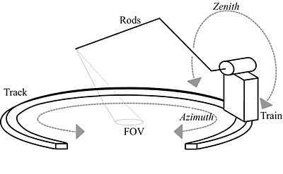
2.1. Original Goniometric Setup
2.2. Improvements
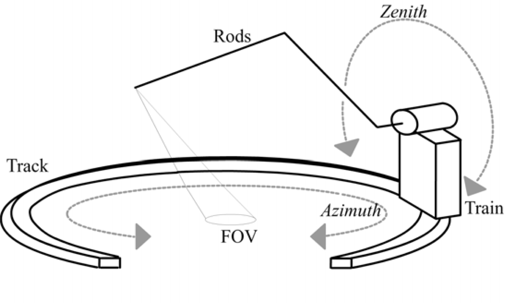
2.2.1. Automated Control
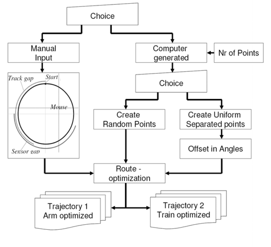
2.2.2. Viewing Angles
2.2.3. Operational calibration
2.3. Sensors
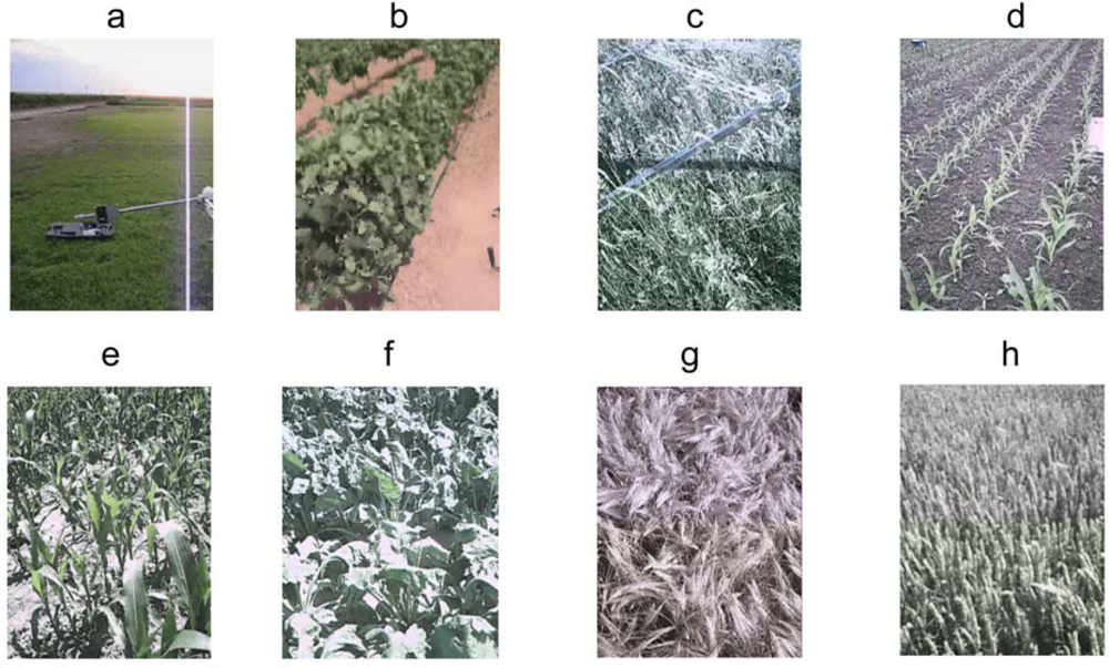
2.4. Fieldsites
3. Results and Discussion
3.1. Within-species Differences in Canopy Structure
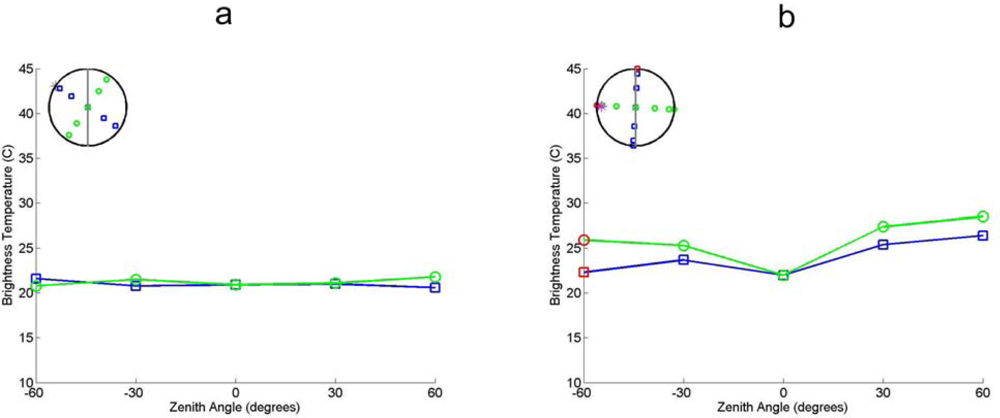
3.1.1. Grass
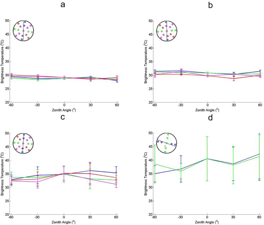
3.1.2. Maize
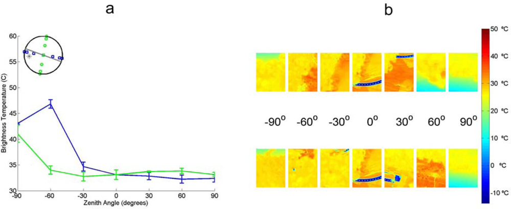
3.2. Inter-species Differences in Canopy Structure
3.3. Discussion
4. Conclusions
Acknowledgments
References and Notes
- Jiménez-Muñoz, J.C.; Sobrino, J.A.; Gillespie, A.; Sabol, D.; Gustafson, W.T. Improved land surface emissivities over agricultural areas using ASTER NDVI. Remote Sens. Environ 2006, 103, 474–487. [Google Scholar]
- Gitelson, A.A.; Wardlow, B.D.; Keydan, G.P.; Leavitt, B. An evaluation of MODIS 250-m data for green LAI estimation in crops. Geophy. Res. Lett 2007, 34, L20403. [Google Scholar] [CrossRef]
- Su, Z. The Surface Energy Balance System (SEBS) for estimation of turbulent heat fluxes. Hydrol. Earth Syst. Sci 2002, 6, 85–99. [Google Scholar]
- Su, Z.; Pelgrum, H.; Menenti, M. Aggregation effects of surface heterogeneity in land surface processes. Hydrol. Earth Syst. Sci 1999, 3, 549–563. [Google Scholar]
- Giorgi, F.; Avissar, R. Representation of heterogeneity effects in earth system modeling: experience from land surface modelling. Rev. Geophys 1997, 35, 413–437. [Google Scholar]
- Yamaguchi, Y.; Kahle, A.B.; Tsu, H.; Kawakami, T.; Pniel, M. Overview of Advanced Spaceborne Thermal Emission and Reflection Radiometer (ASTER). IEEE Trans. Geosci. Remote Sen 1998, 36, 1062–1071. [Google Scholar]
- Milton, E.J.; Schaepman, M.E.; Anderson, K.; Kneubühler, M.; Fox, N. Progress in field spectroscopy. In Remote Sens. Environ; 2007. [Google Scholar] [CrossRef]
- Verhoef, W. A Bayesian optimization approach for model inversion of hyperspectral-multidirectional observations: the balance with a priori information. Proceedings of the 10th International Symposium of Physical Measurements and Spectral Signatures in Remote Sensing, Davos, Switzerland, March 12–14, 2007; pp. 208–213.
- Gobron, N.; Pinty, B.; Verstraete, M.M.; Martonchik, J.V.; Knyazikhin, Y.; Diner, D.J. Potential of multiangular spectral measurements to characterize land surfaces: conceptual approach and exploratory application. J. Geophys. Res 2000, 105, 17539–17549. [Google Scholar]
- Knyazikhin, Y.; Martonchik, J.V.; Diner, D.J.; Myeni, R.B.; Verstraete, M.M.; Pinty, B.; Gobron, N. Estimation of vegetation canopy leaf area index and fraction of absorbed photosynthetically active radiation from atmosphere-corrected MISR data. J. Geophys. Res 1998, 103, 32239–32256. [Google Scholar]
- Tang, S.; Chen, J.M.; Zhu, Q.; Li, X.; Chen, M.; Sun, R.; Zhou, Y.; Deng, F.; Xie, D. LAI inversion algorithm based on directional reflectance kernels. J. Environ. Manage 2007, 85, 638–648. [Google Scholar]
- Martonchik, J.V.; Bruegge, C.J.; Strahler, A.H. A review of Reflectance nomenclature used in remote sensing. Remote Sens. Rev 2000, 19, 9–20. [Google Scholar]
- Verhoef, W.; Jia, L.; Xiao, Q.; Su, Z. Unified optical - thermal four - stream radiative transfer theory for homogeneous vegetation canopies. IEEE Trans. Geosci. Remote Sen 2007, 45, 1808–1822. [Google Scholar]
- Gastellu-Etchegorry, J.P.; Martin, E.; Gascon, F. DART: a 3D model for simulating satellite images and studying surface radiation budget. Int. J. Remote Sens 2004, 25, 73–96. [Google Scholar]
- Schopfer, J.; Dangel, S.; Kneubühler, M.; Itten, K. The Improved Dual-view Field Goniometer System FIGOS. Sensors 2008, 8, 5120–5140. [Google Scholar]
- Li, Z.-L.; Zhang, R.; Sun, X.; Su, H.; Tang, X.; Zhu, Z.; Sobrino, J.A. Experimental system for the study of the directional thermal emission of natural surfaces. Int. J. Remote Sens 2004, 25, 195–204. [Google Scholar]
- FieldSpec Pro, User Guide; Analytical Spectral Devices, Inc: Boulder, CO, USA, 2000.
- Legrand, M.; Pietras, C.; Brogniez, G.; Haeffelin, M.; Abuhassan, N.K.; Sicard, M. A high-accuracy multiwavelength radiometer for in situ measurements in the thermal infrared. Part 1: Characterization of the instrument. J. Atmos. Ocean. Technol 2000, 71, 1203–1214. [Google Scholar]
- Su, Z.; Timmermans, W.J.; Gieske, A.; Jia, L.; Elbers, J.A.; Olioso, A.; Timmermans, J.; van der Velde, R.; Jin, X.; van der Kwast, H.; Nerry, F.; Sabol, D.; Sobrino, J.A.; Bianchi, R. Quantification of land-atmosphere exchanges of water, energy and carbon dioxide in space and time over the heterogeneous Barrax site. Int. J. Remote Sen 2008, 29, 5215–5235. [Google Scholar]
- Yin, X.; van Laar, H.H. Crop Systems Dynamics: An Ecophysiological Model of Genotype-by-Environment Interactions (GECROS); Wageningen Academic Publishers: Wageningen, 2005. [Google Scholar]
- Timmermans, J.; van der Tol, C.; Verhoef, W.; Su, Z. Contact and directional radiative transfer temperature measurements of sunlit and shaded surface components during the SEN2FLEX 2005 campaign. Int. J. Remote Sen 2008, 29, 5183–5192. [Google Scholar]
- Sobrino, J.A.; Romaguera, M.; Sòria, G.; Zaragoza, M.M.; Gomez, M.; Cuenca, J.; Julien, Y.; Jiménez-Muñoz, J.C.; Su, Z.; Jia, L.; Gieske, A.S.M.; Timmermans, W.J.; van der Kwast, H.; Olioso, A.; Nerry, F.; Sabol, D.; Moreno, J. Thermal measurements in the framework of SPARC. Proceedings of the ESA WPP-250: SPARC final workshop, Enschede: ESA, July 4–5, 2005.
- Painter, T.H.; Dozier, J. Measurements of the hemispherical-directional reflectance of snow at the fine spectral and angular resolution. J. Geophys. Res 2004, 109, D18115. [Google Scholar]
- Schneider, T.; Zimmerman, S.; Menaces, I. Field Goniometer system for Accompanying directional measurements. Proceedings of the 2nd CHRIS/PROBA workshop, Frascati, Italy (ESA SP-578), April 28–30, 2004.
- Van Olden, A.P.; Wiring, J. Atmospheric boundary layer research at Cabauw. Bound-Lay Meteorol 1996, 78, 39–69. [Google Scholar]
- Su, Z.; Timmermans, W.J.; Dost, R.; Bianchi, R.; Gomez, J.A.; House, A.; Hansel, I.; Menenti, M.; Magill, V.; Esposito, M.; Harrick, R.; Bossed, F.; Rother, R.; Blink, H.K.; Vekerdy, Z.; Sobrino, J.A.; van der Tol, C.; Timmermans, J.; van Lake, P.; Salaam, S.; van der Kwast, H.; Classes, E.; Stalk, A.; Jia, L.; Moors, E.; Autogenesis, O.; Gillespie, A. EAGLE 2006 – Multi-purpose, multi-angle and multi-sensor in-situ and airborne campaigns over grassland and forest. Proceedings of the AGRISAR and EAGLE campaigns, final workshop, October 15–16, 2007. ESA/ESTEC, Norwalk, The Netherlands. ESA, (ESA Proceedings WPP-279)..


| Accuracy (K) | Spectral Res. (K) | IFOV° | Specifics | |
|---|---|---|---|---|
| Thermal Radiometers | ||||
| CIMEL 312-1 | ±0.5 | 0.05 | 10 | 4 Bands |
| CIMEL 312-2 | ±0.5 | 0.05 | 10 | 6 Bands |
| Everest 3000 | ±0.5 | 0.10 | 20 | broadband |
| Thermal Cameras | ||||
| Thermal Irisys 1010 | ±0.5 | 0.10 | 20.0 × 20.0 | 16 × 16 pixels |
| Thermotracer TH9100 Pro | ±2.0 | 0.06 | 21.7 × 16.4 | 320 × 240 pixels |
| Net radiation Optical | Campbell CNR1 |
| Net radiation Thermal | Campbell CNR1 |
| Wind speed | Campbell A100R |
| Wind direction | Campbell W200P |
| Pressure | Campbell PTB101B |
| Humidity | Campbell HMP45C |
| Air temperature | Campbell HMP45C |
| Soil temperature | Campbell 107T |
| Kinematic temperatures | SEMI 833 ET |
© 2009 by the authors; licensee MDPI, Basel, Switzerland This article is an open-access article distributed under the terms and conditions of the Creative Commons Attribution license (http://creativecommons.org/licenses/by/3.0/).
Share and Cite
Timmermans, J.; Ambro Gieske, A.S.M.; Van der Tol, C.; Verhoef, W.; Su, Z. Automated Directional Measurement System for the Acquisition of Thermal Radiative Measurements of Vegetative Canopies. Sensors 2009, 9, 1409-1422. https://doi.org/10.3390/s90301409
Timmermans J, Ambro Gieske ASM, Van der Tol C, Verhoef W, Su Z. Automated Directional Measurement System for the Acquisition of Thermal Radiative Measurements of Vegetative Canopies. Sensors. 2009; 9(3):1409-1422. https://doi.org/10.3390/s90301409
Chicago/Turabian StyleTimmermans, Joris, A.S.M. Ambro Gieske, Christiaan Van der Tol, Wout Verhoef, and Zhongbo Su. 2009. "Automated Directional Measurement System for the Acquisition of Thermal Radiative Measurements of Vegetative Canopies" Sensors 9, no. 3: 1409-1422. https://doi.org/10.3390/s90301409