Article

Observational Studies and a Statistical Early Warning of Surface Ozone Pollution in Tangshan, the Largest Heavy Industry City of North China

1
College of Atmospheric Science, Lanzhou University, Lanzhou, Gansu 730000, China
2
State Key Laboratory of Atmospheric Boundary Layer Physics and Atmospheric Chemistry, Institute of Atmospheric Physics, Chinese Academy of Sciences, Beijing 100029, China
3
Unit 93534 of PLA, Beijing 101212, China
4
College of Material Science, Hebei United University, Tangshan, Hebei 063009, China
*
Author to whom correspondence should be addressed.
Int. J. Environ. Res. Public Health 2013, 10(3), 1048-1061; https://doi.org/10.3390/ijerph10031048
Submission received: 31 January 2013 / Revised: 4 March 2013 / Accepted: 5 March 2013 / Published: 13 March 2013

Abstract

:
Continuous measurements of surface ozone (O3) and nitrogen oxides (NOX) at an urban site (39°37′N, 118°09′E) in Tangshan, the largest heavy industry city of North China during summertime from 2008 to 2011 are presented. The pollution of O3 was serious in the city. The daily maximum 1 h means (O3_1-hr max) reached 157 ± 55, 161 ± 54, 120 ± 50, and 178 ± 75 μg/m3 corresponding to an excess over the standard rates of 21%, 27%, 10%, and 40% in 2008–2011, respectively. The total oxidant level (OX = O3 + NO2) was high, with seasonal average concentrations up to 100 μg/m3 in summer. The level of OX at a given location was made up of NOX-independent and NOX-dependent contributions. The independent part can be considered as a regional contribution and was about 100 μg/m3 in Tangshan. Statistical early warning analysis revealed that the O3 levels would exceed the standard rate by 50% on the day following a day when the daily average ozone concentration (O3_mean) exceeded 87 μg/m3 and the daily maximum temperature (T_max) exceeded 29 °C. The exceed-standard rate would reach 80% when O3_mean and T_max exceeded 113 μg/m3 and 31 °C. Similarly, the exceed-standard rate would reach 100% when O3_mean and T_max exceeded 127 μg/m3 and 33 °C, respectively.

1. Introduction

Ozone (O3) in the lower part of the atmosphere (troposphere) is one of the most widespread global air pollution problems today. Evidence for the adverse effects of O3 on both human health and the environment at existing concentrations can currently be found in many developed countries, as well as developing countries [1,2,3]. Therefore, many countries and regions have established appropriate environmental standards for this pollutant, but human exposure to high concentrations of ground level ozone continues to be a serious problem in many areas in the US and China, despite the implementation of government-mandated emission control strategies [4,5]. The control of ground level ozone is more difficult than for many other primary pollutants because ozone is a secondary pollutant. The formation of ground level ozone depends on the intensity of solar radiation, the absolute concentrations of its precursors such as nitrogen oxides (NOX) and volatile organic compounds (VOCs), and the VOCs/NOX ratios [6,7,8]. Owing to the chemical coupling of O3, nitric oxide (NO), and nitrogen dioxide (NO2), the levels of O3 and NO2 are inextricably linked. Therefore, the response to reductions in the nitrogen oxides emissions is remarkably not linear, and any resultant reduction in the level of nitrogen dioxide is invariably accompanied by an increase in the air concentration of ozone [9,10]. Moreover, the increasing O3 background concentration influences local levels of O3, and NO2 and the efficiency of local emission controls. It is therefore necessary to obtain a thorough understanding of the relationships and the chemical coupling among O3, NO, and NO2 under various atmospheric conditions.
A number of previous studies showed that tropospheric O3 was increasing in many countries and regions [9,10,11,12,13,14]. Recently, many Chinese scientific researchers have monitored and analyzed the pollution of O3 in the northwest, southeast and Beijing-Tianjin-Hebei regions of China [11,13,15,16,17,18,19]. Some studies found that the mountainous northwest area of the Beijing-Tianjin-Hebei region was a storage area for O3, where O3 and OX (=O3 + NO2) levels were remarkably higher than in the Beijing-Tianjin-Hebei plain [15,18], and O3 has become a serious threat to the environment during summertime in certain cities of China. The Beijing-Tianjin-Hebei Atmospheric Environment Monitoring Network was established by the Institute of Atmospheric Physics, Chinese Academy of Sciences (IPA, CAS). The results of the network showed that the complex atmospheric pollution exhibited high concentrations of O3 and fine particles and oxidation in summer, with ubiquitous regional sources [18]. To achieve a reduction in the comprehensive pollution of O3 and particulate matter will be a very serious and difficult challenge in the region [16,18,19].
Tangshan is the largest heavy-industry city with a long history in the Beijing-Tianjin-Hebei regions. Coal emissions and photochemical smog pollution have increased dramatically with the rapid growth of Tangshan’s industrial sector since the 1990s. According to the 2010 Report of the Tangshan Environmental Protection Agency (TEPA), the ambient air quality of Tangshan city has improved gradually in recent years [20]. However, the environmental pollution caused by industrial and transport emissions should not be viewed optimistically. The 2016 International Horticultural Exposition will soon be hosted by Tangshan City, and there is a great need to assess and improve the air quality of the city. Based on the monitoring data from 2008 to 2011, the present study investigated the relationships between ambient levels of O3, NO, NO2, and OX, and developed an early warning assessment method to provide a scientific basis for the prevention of air pollution in Tangshan.

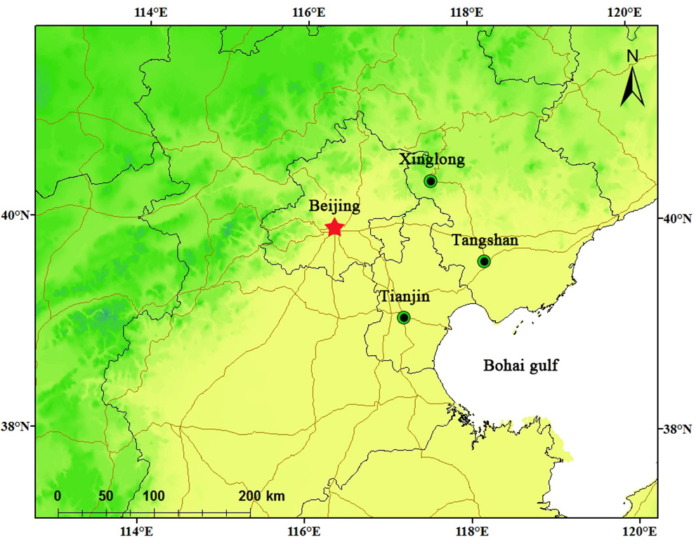
2. Materials and Methods

The data were collected from 2008 to 2011 at the Tangshan station, a site of the Air Quality Monitoring Network, which was established by IPA, CAS and Hebei United University. Figure 1 shows the location of the Tangshan station within the Beijing-Tianjin-Hebei region.
Figure 1. Location of Tangshan station in the Beijing-Tianjin-Hebei region.
Ijerph 10 01048 g001
The station was in the urban center, located on the top of the four-layer office building of Hebei United University (39°37′N, 118°09′E, the air intake was 12 m from the ground). Within a radius of about 5 km of the measured area, the land was relatively flat with some low residential buildings and commercial buildings, without remarkable point emission sources. The station was equipped with the online robotic instruments from Thermo Scientific (Franklin, MA, USA), including a 49I UV photometric O3 Analyzer and 42I NO-NO2-NOX precision chemiluminescence analyzers. Quality control checks, including automatic zero calibration and span checks of gas analyzers, were performed daily, and manual calibrations with standard gases were conducted weekly. Multi-point calibrations of the O3 analyzer used an O3 calibrator (TEI Model 49CPS, Franklin, MA, USA). The NOX analyzers have been zero-checked and span-checked using a zero gas generator (TEI Model 111, Franklin, MA, USA) and an internal O3 source of a multi-gas calibrator (TEI Model 146C, Franklin, MA, USA) with NO standard (National Centre for Standard Materials, Beijing, China). Sampling methods and instrument protocols, as well as quality assurance/quality control (QA/QC) procedures for air quality monitoring, were be executed based on the Chinese National Environmental Protection Standard, Automated Methods for Ambient Air Quality Monitoring. The real-time data was collected and transferred via the internet. The meteorological data were from actual Meteorological Information Comprehensive Analysis and Process System (MICAPS), which was established by the National Meteorological Center of China.

3. Results and Discussion

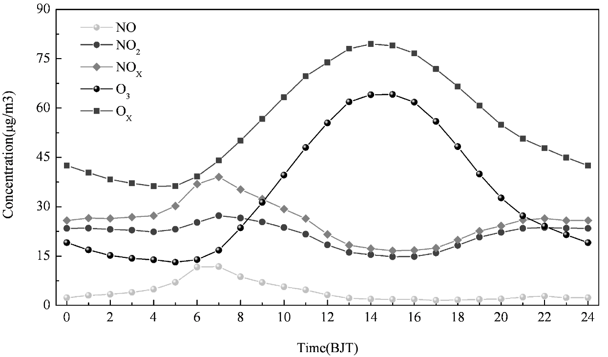
3.1. Variation of O3 in Tangshan during the Summertime

Table 1 shows the mean concentrations of atmospheric pollutants observed in Tangshan during the observation period. Total oxidant was taken to be the sum of O3 and NO2. The daily average (O3_mean), daily maximum 1 h mean (O3_1-h max) and daily maximum 8 h mean (O3_8-h max) were used to describe the changes of O3 concentration. The seasonal average concentrations of O3_mean, O3_1-h max, and O3_8-h max were 69 ± 28, 154 ± 61, and 124 ± 51 μg/m3 in summer during the 4 years study period, respectively. The lowest value of O3_mean was 53 ± 22 μg/m3 in 2010, and the highest was 79 ± 35 μg/m3 in 2011. The result is consistent with a previous study [17]. Xin et al. found that the daily average concentration of O3 were 69 ± 22 μg/m3 in Beijing, 73 ± 16 μg/m3 in its surrounding area (including the Tangshan city), and 100 ± 25 μg/m3 in Xinglong during the Beijing 2008 Olympic Games, respectively [18]. Tang et al. found that were 66 μg/m3 and 54 μg/m3 in Beijing and its surrounding area from July to September during 2001–2006, respectively [16,19]. Compared with the above results, the pollution of O3 was very serious in the city, the same as in Beijing and its surrounding area.
Table 1. The mean concentrations of atmospheric pollutants observed in Tangshan in summer (μg/m3).
PeriodO3NONO2NOXOX
O3_meanO3_1-h maxO3_8-h max
2008: 06/01–09/3075 ± 25157 ± 55129 ± 465 ± 441 ± 1046 ± 13116 ± 27
2009: 07/13–09/3069 ± 29161 ± 54126 ± 527 ± 543 ± 1050 ± 13113 ± 28
2010: 06/01–09/3053 ± 22120 ± 5097 ± 426 ± 547 ± 1354 ± 14100 ± 32
2011: 06/01–08/1079 ± 35178 ± 75143 ± 644 ± 439 ± 1044 ± 12118 ± 36
Mean69 ± 28154 ± 61124 ± 515 ± 543 ± 1149 ± 13112 ± 31
The hourly averaged concentrations of O3, NO, NO2, NOX, and OX are shown in Figure 2. A distinct daily cycle of the pollutants was observed. In general, the daily cycle of O3 reached a peak during the middle of the day and had lower nighttime concentrations. The O3 concentration slowly increased as the sun rose, reached the maximum at 14:00, and then slowly decreased until 05:00 of the next morning. The daily cycle of NO, NO2, and NOX concentration showed morning peaks and evening peaks. It can be seen that nitrogen oxides increased with increasing traffic in the morning and evening. NO is converted to NO2 via the reaction with O3 and during daylight hours, and NO2 is converted back to NO by photolysis, which also regenerates O3 [6,7,21,22]. As long as O3 was present in excess, NO did not rise throughout the day. Since the photolysis rate at nighttime is zero there is net removal of O3 by NO. The daily variation patterns of O3 and OX during the study period were similar.
Figure 2. Daily variation of mean concentrations of O3, NO, NO2, NOX, and OX during the summertime in Tangshan.
Ijerph 10 01048 g002

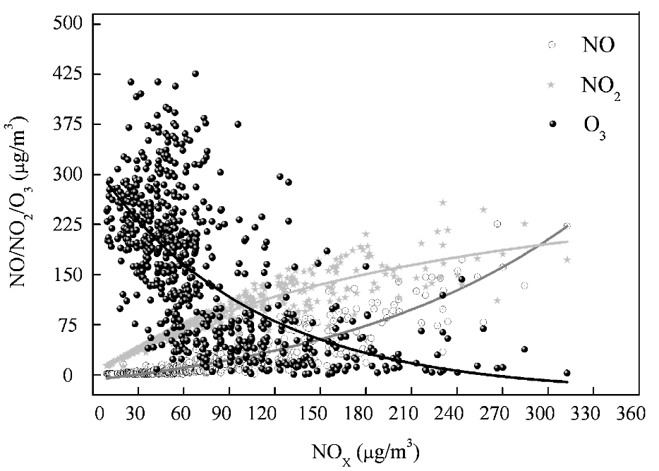
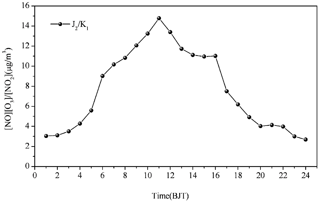
3.2. Chemical Coupling of O3, NO and NO2

Photochemical oxidants play key roles in the atmospheric pollution over urban areas. Among these, O3 and NO2 are important. Produced in the atmosphere through a set of complex reactions [9,10], they are capable of causing adverse impacts on human health and the environment. It is well established that the inter-conversion of O3, NO and NO2 under atmospheric conditions is generally dominated by the following Equations [21,22]:
NO + O3 → NO2 + O2
NO2 + hγ (+O3) → NO + O3
In Equations (1)–(2), NO is initially oxidized by O3 to form NO2 which is then further converted to O3 through photolysis. Moreover, O3 can be consumed by a set of photochemical reactions. In polluted regions, however, peroxy radicals (RO2) participate in Reaction (1) instead of O3 (NO + RO2 → NO2 + RO). Under these conditions, pollution is caused by the accumulation of O3, if the concentration of O3 has reached a certain level. An analysis of the NOX cycle in the atmosphere can contribute to understanding the process of O3 pollution in Tangshan. The previous Equations cycle (1)–(2) allows a determination of the concentrations of these chemical species in this photostationary state, as shown by the following expression [19,21]:
Ijerph 10 01048 i001
In this expression, J2 is the rate of NO2 photolysis and K1 the rate coefficient for the reaction of NO with O3. Coefficient J2 is a function of the solar radiation intensity. Coefficient K1 is a function of the temperature. The variation of the mean values J2/K1 is shown in Figure 3. The range of the mean J2/K1 was from 3 to 15 μg/m3 and the maximum occurred at 11:00.
Figure 3. Daily variation of mean values of J2/K1 (μg/m3).
Ijerph 10 01048 g003
Figure 4. Variation of [NO2]/[OX] as a function of NOX.
Ijerph 10 01048 g004
On the basis of the photostationary state relationship, it is possible to infer an expected variation of daily average [NO2]/[OX] values with [NOX]. The variation of [NO2]/[OX] with NOX concentration is shown in Figure 4. It could be seen that the ratio of [NO2]/[OX] as a function of NOX was higher at night than during day. The greater portion of OX was in the form of NO2 at night. The day and night variation could be explained in terms of variation of the photolysis rate constant (J2), which was a function of the solar radiation intensity and the time required for conversion of NO to NO2 (related to wind speed) [10]. At night O3 and NO cannot coexist and the conversion to NO2 occurs in a short time. Thus, more NOX was speciated as NO2 at night. Further, this showed that the reaction with freshly emitted NO and O3 via the O3 channel mainly controlled NO2 concentration and the O3 remaining after reaction with NO determined O3 concentration. This implied that the contribution of the NOX channel for OX production was major and the radical channel was minor. The residual O3 remaining after the NO-NO2-O3 reaction controlled the O3 concentration in the urban atmosphere during the monitoring period.
The observed variation of daylight average concentrations of O3, NO, and NO2 with the total level of NOX is shown in Figure 5. The lines in Figure 5 were fitted using the multiple regression method to investigate the assumption of a photostationary state. The curves of [O3] and [NO] indicated that the [NOX] crossover point occurred at about 160 μg/m3. When [NOX] < 160 μg/m3, O3 levels were higher than the NO levels, whereas NO dominated at higher [NOX]. The intersection point of the curves represented the two oxidants as [NOX] = 100 μg/m3. When [NOX] < 100 μg/m3 O3 was the dominant form and NO2 dominated at higher [NOX] levels. This pattern was consistent with other research results [10,23,24], although the intersection points vary with local conditions.
Figure 5. Variations of daylight average concentrations of O3, NO, and NO2 with the level of NOX.
Ijerph 10 01048 g005

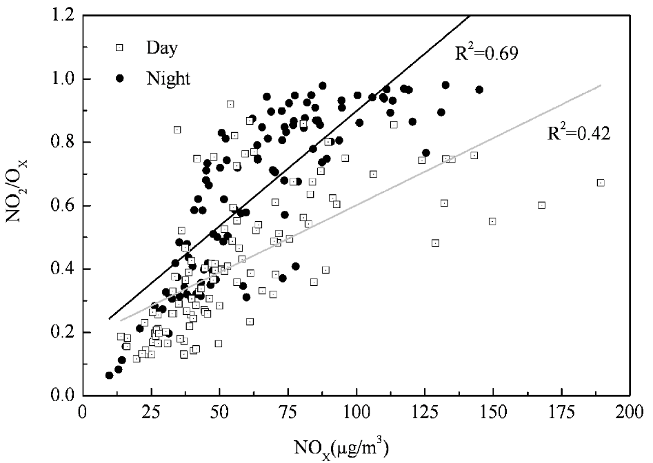
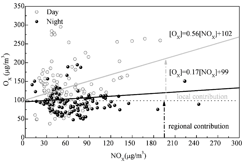
3.3. Local and Regional Contributions to Oxidant

The variation of daylight and nighttime values of OX concentration with the level of NOX are included in Figure 6.
Figure 6. Variation of daily average OX with level of NOX.
Ijerph 10 01048 g006
Total [OX] increased with NOX, where the data were fitted by linear regression. Due to the influence of the photochemical reactions on the formation of O3, there were differences in the values and the linearly fitted equations between daytime and night. It could be observed that the total OX at a given location had an NOX-independent contribution, and an NOX-dependent contribution. The former was effectively a regional contribution which equated to the regional background O3 level, whereas the latter was effectively a local contribution which was correlated with the level of primary pollution. It was found that the NOX-dependent local contribution to OX at nighttime was 25% lower than during the daytime. However, the regional contribution, approximately to 100 μg/m3, was almost equivalent during both day and night. The regional contribution to O3 was highly consistent with the values observed at Xinglong, which is the background station of the Beijing-Tianjin-Hebei region [18]. This result implied that O3 pollution had a similar source throughout the Beijing-Tianjin-Hebei region. It implied that the air quality problem in Tangshan was not only a local problem mainly from street-level pollutions, but also a regional problem from the Beijing-Tianjin-Hebei region. The territorial character of O3 pollution was consistent with the results reported by Xin et al. [18].

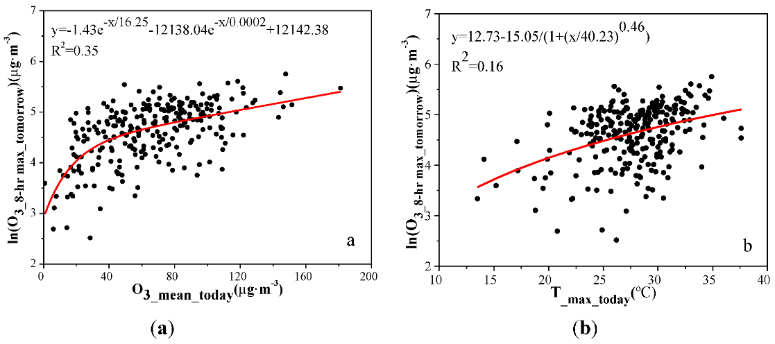
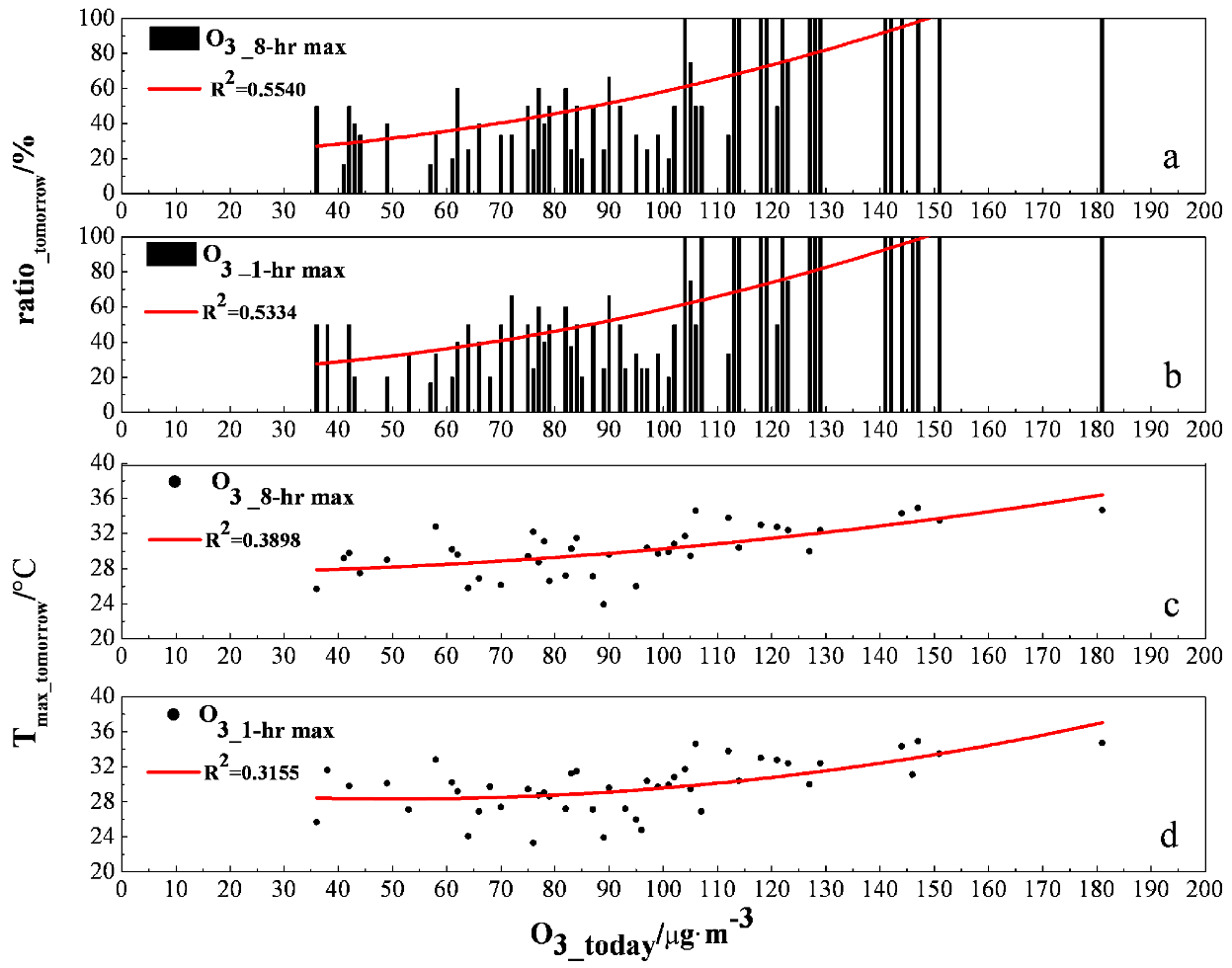
3.4. Ozone Assessment and Early Warning

Based on the National Ambient Air Quality Standards (NAAQS) which will be implemented in 2016 in China, the urban air quality standards of level II for the 1 h average and 8 h average of the O3 concentration were used in this paper. These standards specify a concentration not to exceed 160 μg/m3 and 200 μg/m3, respectively. Table 2 shows the results for the O3 exceed-standard days and exceed-standard rates based on the level II standards. The exceed-standard rates were very high in summer and were 22%, 28%, 10%, and 41% during 2008, 2009, 2010, and 2011, respectively. The highest value (38%) appeared in June, and the lowest value (8.3%) appeared in September. Except in 2010, the number of exceed-standard days during the past 4 years exceeded 25, and the exceed-standard rates exceeded 20% (Table 2). The exceed-standard rates calculated by 8 h average standard were 2.2% higher than those by 1-hour average standard of level II. Therefore, the Tangshan government would need to assume stricter control of O3 pollution over the coming years.
Table 2. Exceed-standard days and exceed-standard rates in Tangshan during the past four years.
2008200920102011Mean
No.RatesNo.RatesNo.RatesNo.RatesNo.Rates
1-h average2521%2127%1010%2740%8323%
8-h average2924%2329%1010%2943%9125%
Mean5422%4428%2010%5641%17424%
Several methods were employed in ozone forecasting in many studies, such as Principal Components Analysis (PCA) which is a statistical technique used to investigate the structure of a data sets [25,26,27,28,29], Artificial Neural Networks (ANN) which is a mathematical model capable of determining a non-linear relationship between two data sets [30,31,32,33], Support Vector Machines (SVM) which have become more popular for air quality prediction [34,35,36], etc. Previous studies had shown that the temperature, humidity, and wind speed can affect the formation of O3, but high temperatures, low humidities and low wind speeds may not have contributed to a high concentration of O3 in all cases [7,37,38,39]. It was also indicated that the formation of O3 was a strongly coupled and complex nonlinear multivariable process [40].
We analyzed the meteorological factors selected to represent the relevant conditions, such as the temperature (T_mean, T_max), dew point temperature (Td_mean), depression of the dew point (Ttd_mean), wind speed (WS_mean), visibility (Vis_mean), 24 h isallobaric value (△P24), and 24 h isallotherm value (△T24). The OX_mean, O3_mean, NO_mean, NO2_mean, NOX_mean, and [NO/NO2] _mean were also introduced in this paper. Table 3 shows the correlation coefficients between the selected factors on the current day and the O3 concentrations at the following day.
Table 3. Coefficients of correlation between 15 factors and O3 concentrations in the next day.
FactorO3_1-h maxO3_8-h max FactorO3_1-h maxO3_8-h max
1T_mean0.38 **0.39 **9△T24−0.01−0.01
2T_max0.45 **0.46 **10OX_mean0.45 **0.45 **
3Td_mean0.28 **0.24 **11O3_mean0.54 **0.57 **
4Ttd_mean0.110.1312NO_mean−0.24 **−0.24 **
5RH_mean−0.12 *−0.14 *13NO2_mean−0.19 *−0.22 *
6WS_mean−0.17 *−0.14 *14NOx_mean−0.27 *−0.27 *
7Vis_mean0.030.0915[NO/NO2]_mean−0.15 *−0.19 *
8△P240.080.09
** Correlation is significant at the 0.01 level (2-tailed); * Correlation is significant at the 0.05 level (2-tailed).
Figure 7 shows 2 two indicators which have been chosen to represent the O3 concentration on the following day. The maximum R-square value observed in these analyses 0.35, was found for O3_mean. The next highest value 0.15, was found for T_max(Figure 7). For all of the functions used in the analysis, the remaining factors had consistently weak effects on the O3 concentration. It implied that O3_mean(X1) and T_max(X2) had more significant effects on the O3 concentration of the next day. A multiple nonlinear regression equation corresponding to these factors was:
Y = 0.005X12 + 0.487X22 − 0.091X1X2 + 2.524X1 − 16.434X2 + 209.977 (R2 = 0.21, P < 0.001).
Figure 7. The changes of O3_8-hr max at the following day in the response to (a) ozone concentration; (b) temperature on the first day during the study periods.
Ijerph 10 01048 g007
Using the multiple nonlinear regression equation, we can estimate the exceed-standard rate of O3 in the next day. Under stable meteorological conditions, when the O3_mean was less than 36 μg/m3 and T_max was less than 24 °C, the next day’s O3 concentration would not exceed the urban air quality standards of level II, the exceed-standard rate at the following day equivalent to 0.
Figure 8 shows the exceed-standard rates of O3 at the following day associated with an increase of 1 μg/m3 on the first day. The figure also indicated the changes of T_max as the concentration of O3 exceeded the standard. An exceed-standard rate of 50% can be defined as the level 1 early warning for O3 pollution, an exceed-standard rate of 80% can be defined as the level 2 early warning for O3 pollution, an exceed-standard rate of 100% can be defined as the level 3 early warning for O3 pollution. The following results were obtained from the curve fitting and statistical analysis used in this study. It showed that under stable meteorological conditions, if O3_mean was less than 36 μg/m3 and T_max was less than 24 °C, the exceed-standard rate at the following day would be 0; if the O3_mean was higher than 87 μg/m3 and T_max was higher than 29 °C, the exceed-standard rate would reach 50%; if the O3_mean was greater than 113 μg/m3 and T_max was greater than 31 °C, the exceed-standard rate would reach 80%; if the O3_mean was greater than 127 μg/m3 and T_max was greater than 33 °C, the exceed-standard rate would reach 100%.
Figure 8. The corresponding exceed-standard ratios at the following day of (a) O3_8-h max and (b) O3_1-h max on the current day, and the corresponding max temperature on the current day when (c) O3_8-h max, and (d) O3_1-h max exceed the standard at the following day.
Ijerph 10 01048 g008

4. Conclusions

Tangshan city is the largest heavy-industry city in North China. In recent decades, the economical development was very rapid, leading to serious air pollution. The observations showed that the concentrations of O3 and OX were very high in summer. The pollution of O3 in Tangshan was not only a local problem resulting mainly from street-level pollution, but also a regional problem from the Beijing-Tianjin-Hebei region. With the statistical analysis of the long-term data, we developed a simple method to assess the exceed-standard rate of O3 at the following day. The short-term early warning method would strengthen the capability to prevent regional atmospheric pollution accidents. In conjunction with other methods, the method could be used to estimate some governmental control strategies for photochemical pollutants in Tangshan city.

Acknowledgments

This work was partially supported by the National Natural Science Foundation of China (41222033, 41021004), the CAS Strategic Priority Research Program Grant (XDA05100102, XDB05020200), the Gong-Yi Program of China Meteorological Administration (GYHY201106034), and the Research Subject of State Science and Technology Support Program of China (2012BAJ18B08).

References

  1. Ramzi, M.K.; James, K. Ozone enhances Diesel Exhaust Particles (DEP)-induced interleukin-8 (IL-8) gene expression in human airway epithelial cells through activation of nuclear factors-kappaB (NF-kappaB) and IL-6 (NF-IL6). Int. J. Environ. Res. Public Health 2005, 2, 403–410. [Google Scholar] [CrossRef]
  2. World Health Organization. Air Quality Guidelines for Particulate Matter, Ozone, Nitrogen Dioxide and Sulfur Dioxide-Global Update, 2005. Available online: http://whqlibdoc.who.int/hq/2006/WHO_SDE_PHE_OEH_06.02_eng.pdf (accessed on 18 December 2012).
  3. Lee, D.S.; Holland, M.K.; Falla, N. The potential impact of ozone on materials in the UK. Atmos. Environ. 1996, 30, 1053–1065. [Google Scholar] [CrossRef]
  4. Duanjun, L.; Remata, S.R.; Rosa, F.; William, R.S.; Quinton, L.W.; Paul, B.T. Sensitivity odeling study for an ozone occurrence during the 1996 Paso Del Norte ozone campaign. Int. J. Environ. Res. Public Health 2008, 5, 181–203. [Google Scholar] [CrossRef]
  5. Roselle, S.J.; Pierce, T.E.; Schere, K.L. The sensitivity of regional ozone modeling to biogenic hydrocarbons. J. Geophys. Res. 1991, 96, 7371–7394. [Google Scholar] [CrossRef]
  6. Tang, X.Y.; Zhang, Y.H.; Shao, M. Chemistry of the Atmospheric Environment(in Chinese), 2nd ed; Higher Education Press: Beijing, China, 2006. [Google Scholar]
  7. Logan, J.A.; Prather, M.J.; Wofsy, S.C. Troposphere chemistry: A global perspective. J. Geophys. Res. 1981, 86, 7210–7254. [Google Scholar] [CrossRef]
  8. Geng, F.H.; Tie, X.X.; Xu, J.M.; Zhou, G.Q.; Peng, L.; Gao, W.; Tang, X.; Zhao, C.S. Characterizations of ozone, NOX, and VOCs measured in Shanghai, China. Atmos. Environ. 2008, 42, 6873–6883. [Google Scholar] [CrossRef]
  9. Lynette, J.C.; Michael, E.J. Analysis of the relationship between ambient levels of O3, NO2 and NO as a function of NOX in the UK. Atmos. Environ. 2001, 35, 6391–6405. [Google Scholar] [CrossRef]
  10. Mazzeo, N.A.; Venegasa, L.E.; Choren, H. Analysis of NO, NO2, O3 and NOX concentrations measured at a green area of Buenos Aires City during wintertime. Atmos. Environ. 2005, 39, 3055–3068. [Google Scholar] [CrossRef]
  11. Wang, S.G.; Zhang, L.; Chen, C.H.; Yuan, J.Y. Retrospect and prospect for the studies of atmospheric environment in the Lanzhou area (in Chinese). J. Lanzhou Univ. 1999, 35, 189–204. [Google Scholar]
  12. Lu, W.Z.; Wang, X.K.; Wang, W.J.; Leung, A.Y.T.; Yuen, K.K. A preliminary study of ozone trend and its impact on environment in Hong Kong. Environ. Int. 2002, 28, 503–512. [Google Scholar] [CrossRef]
  13. Wang, X.S.; Li, J.L.; Zhang, Y.H.; Xie, S.D.; Tang, X.Y. Ozone source attribution during a severe photochemical smog episode in Beijing, China. Sci. Chin. B Chem. 2009, 39, 548–559. [Google Scholar]
  14. Lee, Y.C.; Calori, G.; Hills, P.; Carmichael, G.R. Ozone episodes in urban Hong Kong 1994–1999. Atmos. Environ. 2002, 36, 1957–1968. [Google Scholar] [CrossRef]
  15. Zheng, X.D.; Ding, G.A.; Yu, H.Q.; Liu, Y.; Xu, X.D. Vertical distribution of ozone in the planetary boundary layer at the Ming Tombs, Beijing. Sci. Chin. Ser. D Sci. 2005, 35, 45–52. [Google Scholar]
  16. Tang, G.; Wang, Y.; Li, X.; Ji, D.; Ren, S.; Gao, X. Surface ozone trend details and interpretations in Beijing, 2001-2006. Atmos. Chem. Phys. 2009, 9, 8813–8823. [Google Scholar] [CrossRef]
  17. Wang, X.Y.; Xin, J.Y.; Wang, Y.S.; Feng, X.X.; Zhang, Y.P. Observation and analysis of air pollution in Tangshan during summer and autumn time. Environ. Sci. 2010, 31, 878–885. [Google Scholar]
  18. Xin, J.Y.; Wang, Y.S.; Tang, G.Q.; Wang, L.L.; Sun, Y.; Wang, Y.H.; Hu, B.; Song, T.; Ji, D.S.; Wang, W.F.; et al. Variability and reduction of atmospheric pollutants in Beijing and its surrounding area during the Beijing 2008 Olympic Games. Chin. Sci. Bull. 2010, 55, 1937–1944. [Google Scholar] [CrossRef]
  19. Tang, G.; Wang, Y.; Li, X.; Ji, D.; Gao, X. Spatial-temporal variations in surface ozone in Northern China as observed during 2009–2010 and possible implications for future air quality control strategies. Atmos. Chem. Phys. 2012, 12, 2757–2776. [Google Scholar] [CrossRef]
  20. Tangshan Environmental Protection Agency. Tangshan Environment Bulletin. Available online: www.tshbj.net/portal/manage/manage.action?column=e253b3528d2c467b8c9e362a9b5c6280&article=3358424b72dd4b12afa1f16613e9c5f7 (accessed on 18 December 2012).
  21. Seinfeld, J.H.; Pandis, S.N. Atmospheric chemistry and physics. In Air Pollution to Climate Changes; Wiley: New York, NY, USA, 1998. [Google Scholar]
  22. Leighton, P.A. Photochemistry of Air Pollution; Academic Press: New York, NY, USA, 1961. [Google Scholar]
  23. Lu, K.D.; Zhang, Y.H.; Su, H.; Shao, M.; Zeng, L.M.; Zhong, L.J.; Xiang, Y.R.; Chang, C.C.; Chou, C.K.C.; Andreas, W. Regional ozone pollution and key controlling factors of photochemical ozone production in Pearl River Delta during summer time. Sci. Chin. 2010, 53, 651–663. [Google Scholar] [CrossRef]
  24. Clapp, L.J.; Jenkin, M.E. Analysis of the relationship between ambient levels of O3, NO2 and NO as a function of NOx in UK. Atmos. Environ. 2001, 35, 6391–6405. [Google Scholar]
  25. Lu, W.Z.; He, H.D.; Dong, L.Y. Performance assessment of air quality monitoring networks using principal component analysis and cluster analysis. Build. Environ. 2011, 46, 577–583. [Google Scholar] [CrossRef]
  26. Diamantaras, K.I.; Kung, S.Y. Principal Component Neural Networks: Theory and Applications; Wiley: New York, NY, USA, 1996. [Google Scholar]
  27. Cangelosi, R.; Goriely, A. Component retention in principal component analysis with application to cDNA microarray data. Biol. Direct 2007, 2, 1–21. [Google Scholar] [CrossRef]
  28. Guo, Y.; Schuurmans, D. Efficient Global Optimization for Exponential Family PCA and Low-Rank Matrix Factorization. In Proceedings of Allerton Conference on Communication Control, and Computing, Urbana, IL, USA, 23–26 September 2008.
  29. Olawale, F.; Garwe, D. Obstacles to the growth of new SMEs in South Africa: A principal component analysis approach. Afr. J. Bus. Manag. 2010, 4, 729–738. [Google Scholar]
  30. Corani, G. Air quality prediction in Milan: Feed-forward neural networks, pruned neural networks and lazy learning. Ecol. Model. 2005, 185, 513–529. [Google Scholar] [CrossRef]
  31. Gomez-Sanchis, J.; Martin-Guerrero, J.D.; Soria-Olivas, E.; Vila-Frances, J.; Carrasco, J.L.; Valle-Tascon, S.D. Neural networks for analysing the relevance of input variables in the prediction of tropospheric ozone concentration. Atmos. Environ. 2006, 40, 6173–6180. [Google Scholar] [CrossRef]
  32. Heo, J.S.; Kim, D.S. A new method of ozone forecasting using fuzzy expert and neural network systems. Sci. Total Environ. 2004, 325, 221–237. [Google Scholar] [CrossRef]
  33. Gardner, M.W.; Dorling, S.R. Neural network modelling and prediction of hourly NOX and NO2 concentrations in urban air in London. Atmos. Environ. 1999, 33, 709–719. [Google Scholar] [CrossRef]
  34. Lin, Y.; Lee, Y.; Wahba, G. Support Vector Machines for Classification in Nonstandard Situations; Technical Report 1016 for Department of Statistics, University of Wisconsin: Madison, WI, USA, 2000. [Google Scholar]
  35. Rish, I.; Grabarnilk, G.; Cecchi, G.; Pereira, F.; Gordon, G. Closed-Form Supervised Dimensionality Reduction with Generalized Linear Models. In Proceedings of the International Conference on Machine Learning (ICML), Helsinki, Finland, 5–9 July 2008.
  36. Lu, W.Z.; Wang, D. Ground-level ozone prediction by support vector machine approach with a cost-sensitive classification scheme. Sci. Total Environ. 2008, 395, 109–116. [Google Scholar] [CrossRef]
  37. Xu, X.D.; Shi, X.H.; Xie, L.A.; Ding, G.A.; Miao, Q.J.; Ma, J.Z.; Zheng, X.D. Spatial character of the gaseous and particulate state compound correction of urban atmospheric pollution in winter and summer. Sci. Chin. Ser. DSci. 2005, 35, 53–65. [Google Scholar]
  38. Jacob, D.J. Introduction to Atmospheric Chemistry; Princeton University Press: Princeton, NJ, USA, 1999. [Google Scholar]
  39. Wang, G.C.; Kong, Q.X.; Chen, H.B.; Xuan, Y.J.; Wan, X.W. Characteristics of ozone vertical distribution in the atmospheric over Beijing. Adv. Earth Sci. 2004, 19, 743–748. [Google Scholar]
  40. An, J.L.; Wang, Y.S.; Li, X.; Sun, Y.; Shen, S.H.; Shi, L.Q. Analysis of the relationship between NO, NO2 and O3 concentrations in Beijing. Environ. Sci. 2010, 28, 706–711. [Google Scholar]

