Article

A Comparison of Exposure Metrics for Traffic-Related Air Pollutants: Application to Epidemiology Studies in Detroit, Michigan

1
Department of Environmental Health Sciences, School of Public Health, University of Michigan, 1420 Washington Heights, Ann Arbor, MI 48109, USA
2
National Exposure Research Laboratory, U.S. Environmental Protection Agency, 109 T.W. Alexander Drive, Research Triangle Park, NC 27711, USA
3
Department of Pediatric Pulmonary, Medical School, University of Michigan, 1500 East Medical Center Drive, Ann Arbor, MI 48109, USA
4
Department of Biostatistics, School of Public Health, University of Michigan, 1420 Washington Heights, Ann Arbor, MI 48109, USA
*
Author to whom correspondence should be addressed.
Int. J. Environ. Res. Public Health 2014, 11(9), 9553-9577; https://doi.org/10.3390/ijerph110909553
Submission received: 6 June 2014 / Revised: 25 August 2014 / Accepted: 26 August 2014 / Published: 15 September 2014
(This article belongs to the Special Issue Air Pollution Modeling)

Abstract

:
Vehicles are major sources of air pollutant emissions, and individuals living near large roads endure high exposures and health risks associated with traffic-related air pollutants. Air pollution epidemiology, health risk, environmental justice, and transportation planning studies would all benefit from an improved understanding of the key information and metrics needed to assess exposures, as well as the strengths and limitations of alternate exposure metrics. This study develops and evaluates several metrics for characterizing exposure to traffic-related air pollutants for the 218 residential locations of participants in the NEXUS epidemiology study conducted in Detroit (MI, USA). Exposure metrics included proximity to major roads, traffic volume, vehicle mix, traffic density, vehicle exhaust emissions density, and pollutant concentrations predicted by dispersion models. Results presented for each metric include comparisons of exposure distributions, spatial variability, intraclass correlation, concordance and discordance rates, and overall strengths and limitations. While showing some agreement, the simple categorical and proximity classifications (e.g., high diesel/low diesel traffic roads and distance from major roads) do not reflect the range and overlap of exposures seen in the other metrics. Information provided by the traffic density metric, defined as the number of kilometers traveled (VKT) per day within a 300 m buffer around each home, was reasonably consistent with the more sophisticated metrics. Dispersion modeling provided spatially- and temporally-resolved concentrations, along with apportionments that separated concentrations due to traffic emissions and other sources. While several of the exposure metrics showed broad agreement, including traffic density, emissions density and modeled concentrations, these alternatives still produced exposure classifications that differed for a substantial fraction of study participants, e.g., from 20% to 50% of homes, depending on the metric, would be incorrectly classified into “low”, “medium” or “high” traffic exposure classes. These and other results suggest the potential for exposure misclassification and the need for refined and validated exposure metrics. While data and computational demands for dispersion modeling of traffic emissions are non-trivial concerns, once established, dispersion modeling systems can provide exposure information for both on- and near-road environments that would benefit future traffic-related assessments.

1. Introduction

Residential location and proximity to major roads have been widely used in analyses of exposures and adverse health effects that can result from traffic-related air pollutants, reflecting the elevated concentrations found near busy roads [1,2,3,4,5,6,7,8,9]. As an indicator or exposure surrogate, residential distance to roads, or more generally, residence location, is intended to reflect the portion of exposure received at home, which is generally the dominant share since most individuals spend the majority of their time at home [10]. Residence location or proximity to roads can be used as a surrogate exposure metric itself, or as an input to land use regression, dispersion, space-time (geostatistical), and hybrid models, which are designed to estimate ambient air concentrations and sometimes personal exposures [11,12,13,14,15].
Actual exposure for any particular individual will be the result of many factors, e.g., the amount of time spent indoors and outdoors, building and vehicle cabin air exchange rates, and breathing rates [12]. Unfortunately, direct measurement of traffic-related air pollutant exposure is rarely practicable due to cost and logistical issues [15]. Ambient air quality monitoring networks do not provide the spatial coverage needed to estimate near-road exposures [13], and personal, home or biomarker measurements rarely are feasible in large scale studies. Still, it remains important to improve exposure estimates that are used in epidemiology, health impact, environmental justice and other studies [1,14,16,17,18]. Improved estimates will minimize exposure misclassification that can bias results of epidemiology studies towards the null [19], incorrectly predict risks in health impact studies, and misidentify affected populations in environmental justice studies.
This paper explores alternate metrics for characterizing exposure to traffic-related air pollutants, including metrics based on proximity to major roads, traffic volume and density, traffic type, traffic emissions density, and pollutant concentrations from dispersion modeling. These metrics are being utilized in an ongoing epidemiology study investigating effects of diesel exhaust emissions on the respiratory health of asthmatic children in Detroit, MI, USA [20]. The evaluation of the exposure metrics presented in this paper includes a comparison of exposure distributions, spatial variability using maps coded by exposure group, intraclass correlations, and concordance rates.

2. Methods

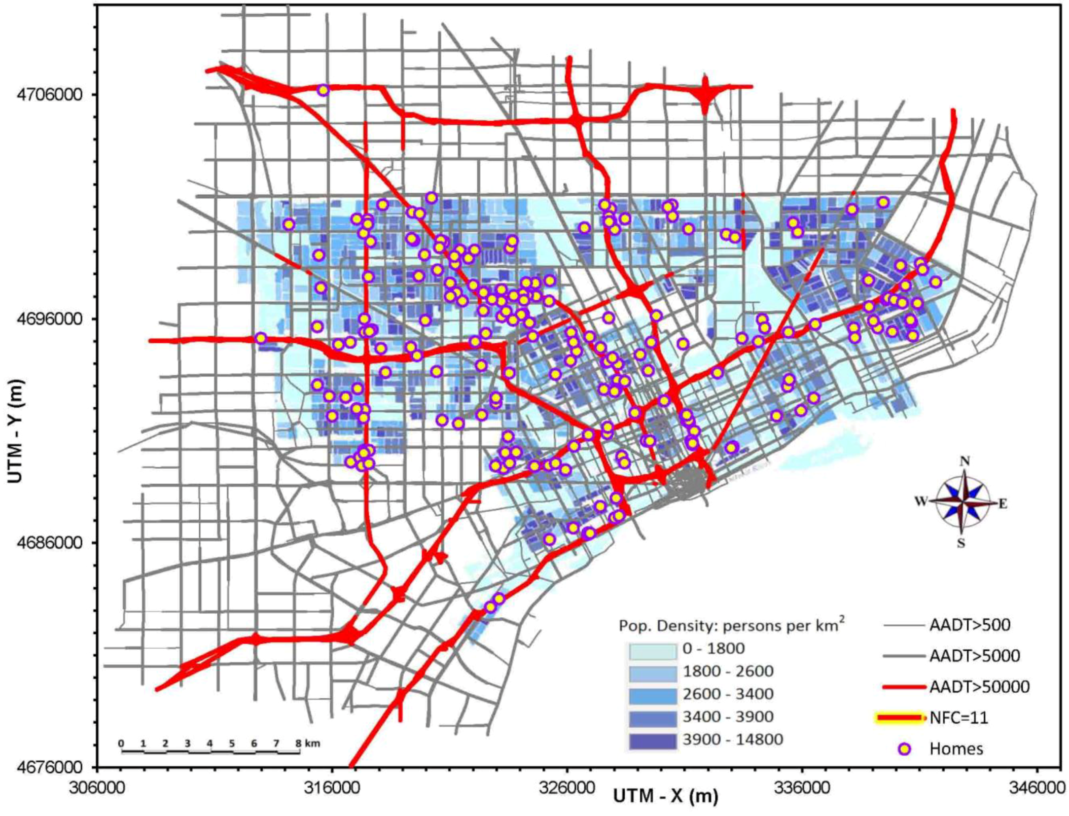
2.1. Study Population

The Near-road EXposures and effects of Urban air pollutants Study (NEXUS) was designed to examine near-roadway exposures to air pollutants and respiratory health in children with asthma living near major roads in Detroit, MI. This community-based participatory research (CBPR) study was designed and conducted with community input and consent. Children with asthma or symptoms of asthma from 6 to 14 years of age were recruited on the basis of the proximity of their home to major roads in three traffic categories: high diesel/high traffic (HDHT), defined as homes within 175 m of roads with >6000 commercial vehicles/day (commercial annual average daily traffic; CAADT) and >90,000 total vehicles/day (annual average daily traffic; AADT); low diesel/high traffic (LDHT), defined as homes within 175 m of roads with >90,000 AADT and <4500 commercial vehicles/day; and low diesel/low traffic (LDLT) homes located >300 m from roads with >25,000 AADT and greater than 500 m from roads with >90,000 AADT. In the initial groups, the designation of commercial vehicles was used as a surrogate for diesel vehicles. Children in the LDLT group were drawn from the same neighborhoods and school catchment areas as the other groups, but lived further from high-traffic corridors, thus minimizing possible confounding from unmeasured neighborhood-associated covariates.
Ultimately, 139 children were recruited and participated in the study from September 2010 to December 2012. Because a number of children moved during the study, a total of 218 residence locations were considered (Figure 1). The study population had approximately equal distribution across the three traffic categories. The population was primarily minority (non-Hispanic Blacks constituted 82% of the participants, Hispanics 8%, non-Hispanic Whites 4%, and other/multiracial 6%). Many households were poor (about one-third of families reported annual household incomes below $15,000).

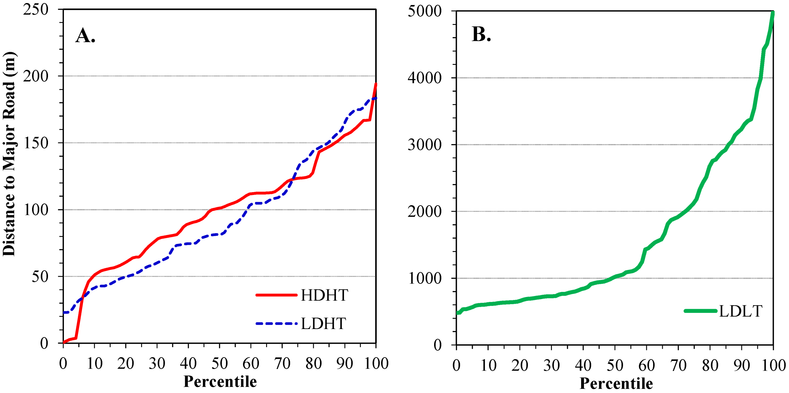
2.2. Residential Proximity to Major Roadways

Because concentrations of traffic-related air pollutants rapidly decrease with distance from roads, considerable effort was spent to obtain accurate estimates of home locations and the distance to major road. Initially, to guide field staff in their recruitment efforts, candidate homes were identified using GIS-produced maps, which identified buffers within 200 m of selected highways and the street and house numbers of residences within these buffers. For the children recruited and enrolled into the study, the resulting 218 home locations were geocoded using three approaches. The first used a hand-held GPS device (60CS, Garmin International Inc., Olathe, KS, USA) operated by our technician who stood as close as possible to the residence’s front door. When the indicated accuracy was <10 m, the location was recorded on a data entry form and as a waypoint in the device’s memory. The calibration of the device was confirmed using several other GPS units. Second, online automated geocoding software provided by “Bing Maps” [21] was used by entering the number, street, city and ZIP code of each residence into this application, which returned latitude and longitude. The Bing Map estimates used the European Petroleum Survey Group (EPSG) code, a Mercator projection, and a spherical model of the earth [22]. The third geocoding estimate used the address locator in the online U.S. Streets Geocode Service in ArcGIS, ESRI ArcMap 10.0 (Redlands, CA, USA). This system uses a cascading sequence of geolocators starting with the Tele Atlas Address Points database, followed by the Tele Atlas Street Address Range database, 9-digit ZIP code, and then the 5-digit ZIP code locators [23].
Figure 1. Map of modeled road network in study area, and locations of 218 homes of participants in NEXUS. Shaded area defines city of Detroit and population by Census Block group. Axis scales are Universal Traverse Mercator coordinates (m). AADT is annual average daily traffic (vehicles/day). Highlighted roads are National Functional Class 11, called high diesel/high traffic roads in NEXUS. Windsor, Canada (not shown), is immediately to the south-east.
Ijerph 11 09553 g001
All coordinates were converted to Universal Traverse Mercator (UTM) coordinates for use in subsequent analyses. If differences between the GPS and automated geocoding coordinates exceeded 100 m, data were checked, plotted, and if needed, our technician was sent out to confirm GPS coordinates a second (and sometimes a third) time, at which point all GPS measurements agreed. Final home locations are plotted in Figure 1. On average, the automated geocoding estimates diverged from GPS measurements at the NEXUS homes by an average 30 ± 23 m, although much larger errors were not infrequent, e.g., 75th and 95th percentile errors were ~50 and 75 m [24]. The bigger errors can represent a large fraction of the buffer width (200 m) used in the proximity metrics, suggesting that a fraction of homes geocoded using automated systems would be misclassified by such surrogate exposure metrics, especially since automated geocoding programs typically give larger errors than those found for Detroit [15,24].
Distances from each residence to the nearest roads and highways were determined using ESRI ArcMap (version 10.0) “NEAR” function within the Proximity toolset, the 2012 Topologically Integrated Geographic Encoding and Referencing (TIGER) 2012 road shape files, and the North American Datum (NAD) for 1983. A second measure of distance to the nearest highway was calculated using the link-based road network for the emissions inventory described next. This distance averaged 20 m greater than the TIGER estimate, representing the distance to the road centerline rather than to the road edge.

2.3. Road Network, Traffic Data and Emissions Inventory

The modeled road network used 9701 links (linear segments) to represent 3109 km of roads, which included all but the smaller and numerous local roads in the ~800 km2 study area (Figure 1). Major roads (e.g., freeways) were represented using separate links for each direction, large service roads, if any, and ramps. Road network data obtained from the Southeast Michigan Council of Governments (SEMCOG) included the locations, number of lanes, and roadway type (e.g., freeway, arterial). The road network extended at least 5 km beyond the locations of the NEXUS homes, and fully encompassed the city of Detroit (area of ~355 km2).
Hourly vehicle traffic volume and speed on each link were estimated using the SEMCOG Travel Demand Forecast Model, which used a TransCAD-based suite of applications, and temporal profiles for monthly, weekly and daily flows by vehicle class (e.g., heavy-duty diesel, light-duty gasoline). Where possible (e.g., for interstates), estimated vehicle flows were checked against observed traffic counts.
Estimates of total and diesel vehicle volumes on major roads formed the basis of the initial participant recruitment and the exposure classification. The initial grouping of roads (as HDHT, LDHT and LDLT) used 2006 and 2007 maps with AADT and CAADT flows prepared by the Michigan Department of Transportation [25]. As described earlier, subsequent analyses used state and regional data and a traffic demand model to derive AADT for each road link for the year 2010. Traffic on the major road closest to each HDHT and LDHT residence was estimated by summing AADT values on the corresponding road-links, which included at least two links (one for each direction) and occasionally additional links if the road split or if ramps added to the road’s traffic in the vicinity of the residence. At three homes, two major roads had similar proximity and both were counted in the AADT estimate. The corresponding number of lanes on these roads was summed as another measure of road size. Finally, the number of diesel vehicles on the closest major road was calculated as the product of the AADT (vehicles/day) and the fraction of diesel vehicles for the road type, which was 5.23% for “other freeways” (National Functional Class or NFC 12) and 9.18% for interstates (NFC 11). These fractions represent the sum of light-duty diesel trucks, heavy-duty diesel trucks, and heavy-duty diesel vehicles (LDDV, LDDT, HDDV) as derived using state-level data from the U.S. Federal Highway Administration [26], and the U.S. EPA Emission Inventory Improvement Program [27].
Primary mobile source emissions of particulate matter below 2.5 µm dia (PM2.5), oxides of nitrogen (NOx), carbon monoxide (CO) and other pollutants were estimated for each link on an hourly basis, thus producing a spatially and temporally resolved mobile source emissions inventory. The link-based inventory used emission factors representative of each vehicle class in the study area for the year 2010 calculated using the MOVES2010a model with inputs including the average speed and flow on each link, local vehicle mix and age distribution, ambient temperature, season, and road type [28,29]. Due to large uncertainties, particulate emissions for brake and pavement wear, and resuspension of dust were not included in the PM emissions estimates.
Emissions-based exposure metrics incorporate the quantity of traffic-related pollutant emissions released, providing an exposure metric that may be particularly relevant to policies addressing emission controls, transportation control measures, and other actions that directly affect emissions. Emissions density (g/day) was estimated as the daily vehicle exhaust emissions within a 300 m buffer around each home. PM2.5, NOx and CO emissions were considered.

2.4. Concentration Estimates and Dispersion Modeling

We evaluated whether simple “box” models using the emissions density information discussed above could provide useful estimates of near-road pollutant concentrations. We assumed a wind speed u = 3.66 m/s (the long term Detroit average), a mixing height h = 100 m, and the average traffic-related PM2.5 emission rate Q in the 300 m buffer (r = 300 m) around high traffic homes. Concentrations were calculated as C = Q/(2 × u × r × h).
Hourly pollutant concentrations for the year 2010 were predicted at each home for three cases: annual average concentrations due to on-road exhaust emissions; the maximum 24-h concentration also due to on-road exhaust emissions, and the “total” annual average concentration due to on-road, non-road and background sources. Each case used the road-link emissions inventory for the Detroit area described above, the new RLINE dispersion model specifically designed for roadway emissions [30,31], and hourly meteorological data from the Detroit City airport processed by AERMET. RLINE is a steady-state Gaussian formulation for near-surface releases with dispersion parameters that can simulate low wind meander conditions. (The model is available from the U.S. Environmental Protection Agency [32]. The third case used a hybrid model system that integrated RLINE, the ERMOD model for area and point sources in the region (including Canada) using source locations, emission rates and other parameters from the 2008 National Emissions Inventory (NEI), and estimated regional (background) concentrations determined using the Community Multiscale Air Quality (CMAQ) model, observations from air quality monitoring networks in the region, and a space/time kriging model. As described elsewhere in this issue [31], this system is highly flexible, and model outputs can provide spatial and temporal patterns of air pollutants by source category.
Detailed descriptions and evaluations of RLINE and the other dispersion models have been presented elsewhere [30,31,33,34,35]. In Detroit, model results have been compared to ambient observations collected in both routine monitoring networks (AQS) and during the NEXUS intensive campaign. Compared to AQS data, 24-h average PM2.5 concentrations correlated well (0.78 < r < 0.94) with 2010 data collected at four PM2.5 monitoring sites in Detroit, and most predictions were within a factor of two of observations. NOx concentrations predicted at the sole AQS monitoring site in Detroit reproduced morning and afternoon peaks but overpredicted the concentrations, likely due to contributions from regional sources since this site was several km from major highways. Compared to black carbon measured outside of 25 of the NEXUS homes and NOx measured at 9 homes in (September–November) 2010, a pollutant often specific to traffic-related emissions, the model generally captured the magnitude and dynamics of observed concentrations, although concentrations were overpredicted or missed at some sites and some specific hours, likely due to uncertainty in hourly traffic activity and emissions at the road link level. Further description of the evaluation of the modeling system in the Detroit application is presented elsewhere [35].

2.5. Data Analysis

Descriptive analyses included graphs of distributions stratified by the original HDHT, LDHT and LDLT groups. Differences in means between the HDHT and LDHT groups were evaluated using t-tests, and difference in distributions for the same groups were evaluated using the non-parametric Mann-Whitney (MW) tests. (Sample size n = 96 in all cases for both tests). Comparisons between exposure metrics used Spearman’s and Kendall’s τ-b correlation coefficients. The latter correlation coefficient measures interclass agreement by considering the number of concordant pairs of observations minus the number of discordant pairs, expressed as the fraction of total pairs, and accounts for ties. Both are non-parametric measures that range from −1 to 1.
Additional measures of concordance/discordance rates were derived for exposures divided into “high”, “medium” and “low” categories to provide estimates potentially relevant to exposure misclassification, as discussed in the text. The first measure was defined as the percentage of homes identically classified after grouping each metric into tertiles (high, medium and low categories). Thus, 100% agreement indicates that each home is placed in the same tertile for the pair of metrics considered, while random assignment would be expected to yield 33% agreement. For distance, tertiles were reversed, i.e., the shortest distances (presumably the highest exposure) were placed in the third tertile. The skewness of several metrics produced non-uniform tertile ranges, i.e., for the number of lanes (0–6, 6–8 and 8–14), PM2.5 emissions (0–306, 306–1837, 1837–4027 g/day), 24-h peak (6–14, 14–18, 18–47 µg/m3) and annual average (0.8–1.6, 1.6–2.7, 2.7–9.4 µg/m3) PM2.5 concentrations. Thus, another concordance measure was used to examine agreement between “thirds,” defined using three evenly spaced bins between the metric’s minimum and a nominal maximum value, either the actual maximum or an adjusted value that provided at least 15 observations in the top third. This gave ranges for the distance metric of 3067–5025, 1534–3067 and 1–1534 m (reversed); 0–1300, 1300–2600 and >2600 g/day for PM2.5 emissions; 0.8–1.6, 1.6–2.7 and >2.7 µg/m3 for annual average PM2.5 concentrations; and 6–17, 17–27 and >27 µg/m3 for peak 24-h PM2.5 concentrations (Figure 3D, shown in section 3.2, illustrates differences between tertiles and thirds). Again, 100% agreement denotes that the pair of metrics placed each home at the same (low, medium or high) level.

3. Results

3.1. Grouping of Homes by Distance to Roads

By design, many of the children participating in NEXUS lived close to major roads. Most children in the high traffic groups (HDHT and LDHT) lived near one of two interstate highways or two State of Michigan highways: I-75 (n = 30 residence locations), I-94 (n = 20), M10 (n = 30), and M-39 (n = 16). A few children lived near I-96 (n = 3), which was classified as a “medium” diesel high traffic road and not considered further in the present analysis.
The distributions of distances from high traffic roads for the HDHT, LDHT and LDLT groups are shown in Figure 2. Means and distributions in the two high traffic groups did not differ (t-test: p = 0.641; MW test: p = 0.376), and the mean distance was 96 ± 45 m from the road edge. The distributions were rectangular (uniform) in nature, and one residence was as close as 1 m from the road edge (along I-75 in southwest Detroit). In contrast, distances in the LDLT group were much longer, averaging 1,562 ± 1,133 m (±standard deviation).
Figure 2. Distribution of distances of homes to major roads for the three traffic exposure groups. (A) HDHT (high diesel/high traffic) and LDHT (low diesel/high traffic) homes; (B) LDLT (low diesel/low traffic) homes. Based on GPS home location and road edge.
Ijerph 11 09553 g002
Among the HDHT and LDHT groups, distances from roads did not vary among the four major roads (Kruskal-Wallace test, p = 0.628), although the average distance for M-39 was 10 m less than those for the three other major roads. No general trends were noted for residence-road distances with respect to region of the city or distance from downtown.
Exposure metrics such as the proximity to roads, as well as metrics based on traffic activity and dispersion modeling that are discussed later, depend on the accuracy of geocoding for home and other locations, and the positional accuracy of the road network. The latter depends on many factors, including the representation of the road network, e.g., as road edges as used in the preceding analysis, or as links that represent the road centerline as used later with line source dispersion models. Both road shape files and road-link network generally closely matched detailed maps and photographs, however, discrepancies for road-links increased at road sections that were curved since link-based networks simplify geometry using a minimal number of linear segments. Such positional errors can lead to exposure misclassification, particularly for locations very near (e.g., within 20 to 50 m) of major roads.

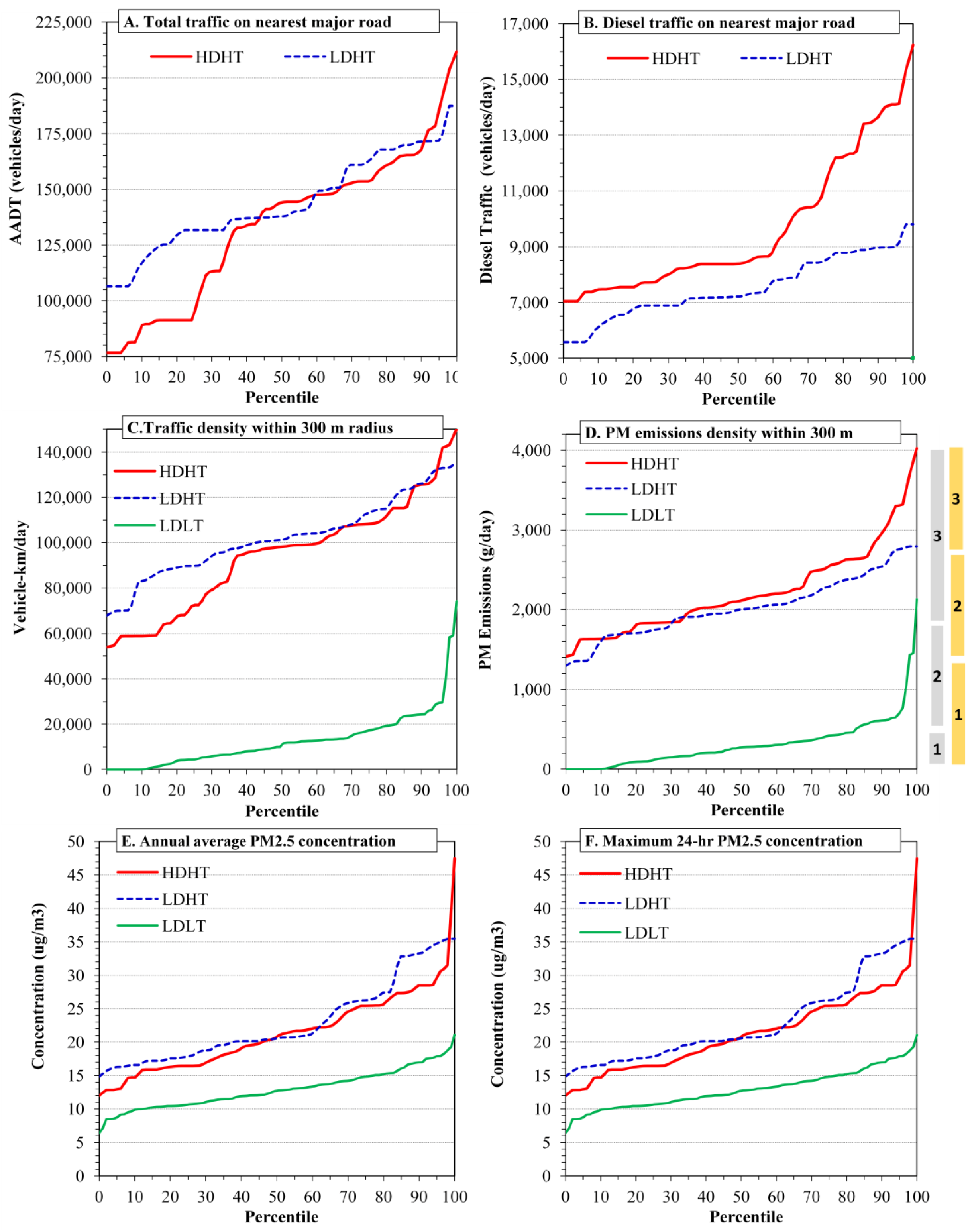
3.2. Total and Diesel Traffic Metrics

The distributions of total and diesel traffic volume on major roads near the NEXUS homes are shown in Figure 3A,B and mapped in Figure 4A,B; descriptive statistics are in Table 1.
As anticipated, diesel vehicle traffic was highly correlated to the total traffic (r = 0.93), however, there are important differences, as discussed below. The maps show the clustering of high traffic homes along five major highways: HDHT homes fall mostly in the south and east along I-75 and I-94 (red circles, Figure 4A); LDHT homes are mostly in the north and west along M10 and M39 (blue circles). The LDLT homes (green circles) are distributed throughout the region.
Table 1. Statistics of AADT volume, diesel traffic volume, and number of lanes for the nearest highways at the high traffic (HDHT and LDHT) homes. Maximum values are affected by the three homes had equal distance to two highways (both were counted).
StatisticAll Traffic (Vehicles/Day)Diesel Traffic (Vehicles/Day)Number of Lanes
HDHTLDHTAllHDHTLDHTAllHDHTLDHTAll
Average133,737 143,965 138,638 9663 7529 8640 7.86.67.2
St. Dev.34,962 21,614 29,634 2510 1130 2237 1.81.11.6
Minimum76,723 106,508 76,723 7043 5570 5570 666
25th Percentile94,202 131,718 124,586 7716 6889 7182 666
Median144,013 137,845 140,722 8386 7209 8218 866
75th Percentile153,576 162,808 160,968 11,297 8515 8974 978
95th Percentile185,442 171,849 180,417 14,098 8988 13,711 11910
Maximum 211,750 187,373 211,750 16,235 9800 16,235 141014
Number504696504696504696
Considering the total traffic (AADT) near the high traffic homes, the average volume was 134,000 ± 30,000 vehicles/day and the average number of lanes was 7.2 ± 1.6. As noted above, three homes were equally near two major roads, including the home with the highest AADT, which was located at the I-94‒M-10 intersection (AADT = 212,000 vehicles/day, counting both roads); the two other homes were at the I-94‒I-96 and I-75‒I-96 junctions (178,000 and 134,000 vehicles/day, respectively). Traffic volumes at such junctions can be difficult to estimate given the numbers of ramps and highway segments involved. Otherwise, the traffic volume estimates were due to a single road. The AADT distributions for HDHT and LDHT homes were similar (t-test: p = 0.091; MW test: p = 0.262; Figure 3A), although the HDHT group had a greater range and its lowest tertile had 25,000 fewer vehicles/day. AADT had negligible correlation with the home’s distance to the road (r = −0.006). The maps suggest that each road had a wide range of traffic volumes, i.e., no apparent geographic bias.
Figure 3. Distributions of selected exposure metrics coded by home group (HDHT = high diesel/high traffic; LDHT = low diesel/high traffic; LDLT = low diesel/low traffic). (A) Total traffic volume on major roads nearest home; (B) Diesel traffic volume on major roads nearest home; (C) Traffic density for roads within 300 m of home; (D) PM2.5 emissions density for roads within 300 m of home; (E) Annual average PM2.5 concentrations due to on-road emissions; (F) Maximum 24-h average PM2.5 concentrations due to on-road emissions. Panel D depicts differences between tertiles (in grey) and thirds (in orange).
Ijerph 11 09553 g003
Figure 4. Depiction of selected exposure metrics mapped by home group (HDHT = high diesel/high traffic; LDHT = low diesel/high traffic; LDLT = low diesel/low traffic). (A) Total traffic volume on major roads nearest home; (B) Diesel traffic volume on major roads nearest home; (C) Traffic density for roads within 300 m of home. (D) PM2.5 emissions density for roads within 300 m of home; (E) Annual average PM2.5 concentrations due to on-road emissions; (F) Maximum 24-h average PM2.5 concentrations due to on-road emissions. In (A) and (B), LDLT homes are shown as green circles without coding for traffic volume.
Ijerph 11 09553 g004
Considering diesel traffic near the high traffic homes, the volume averaged 8640 ± 2240 vehicles/day, and eight homes had over 12,500 diesel vehicles/day. HDHT homes had an average of 2100 diesel vehicles/day more than LDHT homes, a statistically significant difference (t-test: p < 0.001; MW test, p < 0.001). Still, the distributions of HDHT and LDHT homes had considerable overlap, and roughly half of the two sets of homes had a comparable range of diesel volume (7000–9000 vehicles/day; Figure 3B). The highest diesel volume occurred for homes along I-75, while homes along the eastern portion of I-94 had lower diesel traffic volumes than other HDHT homes (Figure 4B). This resulted in part from reclassifying this section of I-94 to an “other highway” (NFC 12) designation rather than “interstate” in an attempt to better match the observed traffic classification. Diesel volume had negligible correlation with distance to the road (r = 0.001). Overall, estimates of diesel traffic are less certain than those for total traffic due to the variation in fleet mix and the limited classification data available.
By design, the LDHT homes were intended to have commercial annual average daily traffic (CADT) below 4500 vehicles/day. There are several reasons for differences between the initial groupings and those computed using the road-link network. First, not all diesel traffic is “commercial” (and vice versa). Based on the fleet composition data used, the bulk of diesel traffic on major roads are heavy duty diesel vehicles (HDDV), which represent 84% of the diesel volume on interstates, and 71% on “other highways”. The balance of diesel vehicles is contributed by light duty diesel vehicles (LDDV) and light duty diesel trucks (LDDT), which respectively represent 11% and 6% of the diesel vehicles on interstates, and 20% and 9% on other highways. With the exception of the 6% to 9% of the diesel vehicles classified as LDDVs, most LDDTs and all HDDVs form part of CADT. With the LDDV fraction removed, differences between the HDHT and LDHT categories slightly increase, e.g., the average volume of diesel traffic is 8700 ± 2,500 vehicles/day near the HDHT homes, and 6300 ± 950 vehicles/day near the LDHT homes. Second, CADT will include some gasoline-powered vehicles. However, the emissions inventory classifications do not correspond well to the AADT/CADT classifications. Third, the initial and road-link estimates of CADT used different data sources: the former depended on local measurements, while the latter used a mix of local, Michigan and national-level data.

3.3. Traffic Density Metric

A measure of traffic density, the number of vehicle-km traveled (VKT) per day within a 300 m radius of each home, was calculated using the road-link network. The average VKT/day was 94,200 ± 24,900 for HDHT homes, 102,200 ± 17,230 for LDHT homes, and 12,700 ± 12,400 for LDLT homes. Differences in traffic density between HDHT and LDHT homes approached statistical significance (t-test: p = 0.071; MW test, p = 0.117; Figure 3C). This metric varied considerably within each home group, e.g., the range spanned a factor of 2.8 for HDHT homes, and variation for homes along the same highway could be considerable, e.g., the southwest section of I-75 has several HDHT homes with low traffic density (Figure 4C). Of the LDLT homes, 4% (n = 4) had moderately high traffic density (41,000 to 74,000 VKT/day), overlapping or nearly overlapping the high traffic homes. Based on this exposure metric, the LDHT homes had slightly greater exposure than HDHT homes.
For most high traffic homes, the largest share by far of the traffic density metric was contributed by interstates and other highways. This exposure metric can be very sensitive to the distance criterion since roads will drop out as the distance criterion (buffer size) decreases. For example, a 150 or 200 m buffer excluded the nearby highway for a few HDHT homes, dropping the KMT/day to nearly zero, despite large values obtained with the 300 m buffer.

3.4. Emissions Density Metrics

Figure 3D and Figure 4D show the PM2.5 emissions density distributions and levels at each home. For PM2.5, the emissions density averaged 2,226 ± 568 g/day at HDHT homes, 2029 ± 379 at LDHT homes, and only 315 ± 320 at LDLT homes. The distributions of PM2.5 emissions near HDHT and LDHT homes appeared similar, although outliers caused results of the statistical tests to vary (t-test: p = 0.052; MW test: p = 0.153), e.g., a few HDHT homes near intersections of major roads (e.g., I-95 and I-75) had very high emissions. For the high traffic homes, nearby highways contributed the bulk of emissions. Emissions rates in the 300 m buffers around LDLT homes were much lower, although a few homes had emissions densities that overlapped those in the high traffic group.
Distributions and maps for NOx and CO emissions density are shown in Supplemental Figures S1 and S2. Results for NOx parallel the findings for PM2.5. However, results for CO diverged as HDHT homes tended to have lower CO emissions within the 300 m buffer, although statistical significance was not reached (t-test: p = 0.072; MW test: p = 0.093). Some of the higher levels were found for homes along M39 (in the western portion of the study region), due to the lower CO contributions from diesel vehicles and the dominance of CO emissions from much more numerous (and gasoline-powered) automobiles. Overall, the pattern for CO closely resembled the traffic density metric (Figure 3C and Figure 4C).
Emission-based metrics may be especially relevant for the traffic analysis zones (TAZ) commonly used by metropolitan planning organizations for various purposes, although TAZs may be relatively large relative to the spatial variability of traffic-related air pollutants. Emission-based metrics can be developed for the major road nearest point of interest (e.g., a home), for roads within a local area, or for buffers around points of interest, as presented here. This metric is pollutant-specific and thus can account for differences in fleet mix, technology and transportation control measures (TCMs) that can affect emissions.

3.5. Concentration Metrics

The “box” model using the average emissions density around high traffic homes for PM2.5 (2226 g/day) gave a predicted PM2.5 concentration of 0.12 µg/m3. This low estimate does not account for temporal variation in emission rates (e.g., rush-hour emissions are approximately twice the average rate) or meteorology (e.g., wind speeds near 1 m/s are not uncommon and mixing heights also vary). In addition, some homes had twice the average emission rate, and results will be sensitive to the buffer size and source configuration. The most significant limitation, however, is the validity of the fully mixed assumption near major roads where vertical dispersion of roadway emissions may not reach 100 m. As shown below, dispersion models designed for near-road applications yielded concentrations that were one to two orders of magnitude higher. Thus, while box models have been used at a city-wide or regional level [36], they do not appear useful for near-road applications.
Dispersion modeling results for PM2.5 are summarized in Table 2, and concentration distributions and maps are shown in the bottom panels of Figure 3 and in Figure 4. Considering emissions from local traffic and annual average concentrations, PM2.5 levels at high traffic homes were 1.6 µg/m3 higher than those at LDLT homes, or about twice that at the LDLT homes. Considering 24-h peak concentrations, PM2.5 levels at several HDHT homes were estimated to exceed 40 µg/m3, which is high relative to PM2.5 standards. (Highly elevated concentrations at a few homes are shown as a sharp uptick in Figure 3E,F) (the U.S. National Ambient Air Quality Standards are currently 12 and 35 µg/m3 for annual and 24-h averages, respectively). The average 24-h peak across the high traffic homes was 11 µg/m3 more than levels at the LDLT homes, again about twice the level. Considering the “total” PM2.5 estimated by the hybrid model, regional sources were dominant, contributing about 12 µg/m3 on an annual average basis across the homes. Given the relatively high contribution of PM2.5 by regional sources, the spatial variability due to local sources was significantly reduced, e.g., PM2.5 levels at low and high traffic homes differed by only 10% to 20% (Distributions and maps of total PM2.5 are shown in the Supplemental Materials).
Table 2. Statistics of PM2.5 concentrations (µg/m3) predicted at home of NEXUS participants, classified by exposure group (HDHT = high diesel/high traffic; LDHT = low diesel/high traffic; LDLT = low diesel/low traffic). The hybrid annual average includes on-road, area, point and regional sources.
StatisticOnroad, Annual AverageOnroad, 24-hr PeakHybrid, Annual Average
HDHTLDHTLDLTHDHTLDHTLDLTHDHTLDHTLDLT
Average3.33.21.521.422.812.915.615.613.9
St. Dev.1.21.00.46.36.22.91.41.51.3
Minimum2.22.10.812.014.96.413.313.712.1
25th Percentile2.72.41.316.417.910.714.614.413.0
Median2.93.01.520.820.612.715.415.313.6
75th Percentile3.83.61.625.426.214.816.216.314.4
95th Percentile4.84.82.429.634.717.918.218.616.5
Maximum9.46.43.347.435.421.120.719.219.7
Number504610250461025046102
The distributions of annual average PM2.5 concentrations at HDHT and LDHT homes due to local traffic were very similar (t-test: p = 0.637; MW test: p = 0.523, Figure 3E and Figure S3); peak 24-h concentrations tended to be slightly but not statistically higher at the LDHT homes (t-test: p = 0.251; MW test: p = 0.235; Figure 3E,F). The highest prediction, considered an outlier since it considerably exceeded any other prediction, occurred at a home very near I-75. Excluding this point, concentrations due to local traffic varied by about 3-fold in each exposure group.
Unlike the metrics discussed earlier, dispersion modeling results are expressed as concentrations that permit direct and meaningful comparisons to air quality standards, monitoring data and other studies. For example, a recent application of a hybrid dispersion model in London, England showed annual average PM2.5 contributions from 1 to 5 µg/m3 due to local vehicle exhaust (depending on site), and about 11 µg/m3 due to other local and regional sources [11]. Both the traffic and regional PM2.5 contributions were very similar to those predicted for Detroit. While an intercity comparison incorporating meteorology and spatial factors is beyond the present scope, the volume of traffic and the number of large and high emitting diesel trucks on Detroit’s highways may produce PM2.5 concentrations that are comparable to those in London, despite Detroit’s smaller size and lower fraction of diesel vehicles.

3.6. Comparison of Exposure Metrics

Table 3 compares the exposure metrics using Spearman’s and Kendall’s τ-b correlation coefficients. To include the original categorical proximity classifications in this analysis, LDLT, LDHT and HDHT groups were coded two ways: as 1, 2 and 3 respectively in the “Group1” variable, with the assumption that exposures were ranked as HDHT > LDHT > LDLT; and as 1, 2 and 2 in the “Group2” variable with the assumption that exposures were HDHT ≈ LDHT > LDLT, as suggested by most metrics. Table 3 colors the higher (>0.6 and >0.8, absolute value) correlation coefficients. For the Spearman coefficients, absolute values above 0.17 (n = 96 for comparisons involving only high traffic groups) or 0.12 (n = 198 to 218 for other comparisons) are statistically significant (p < 0.05, 1-sided test). While the measures have some differences, e.g., the Spearman coefficients are 3% to 23% higher than the Kendall τ-b coefficients and contrasts in Kendall’s τ-b coefficients tend to be larger, similar patterns emerge.
The original proximity classifications (“Group1” and “Group2”) are related to distance to the nearest highway (defining variables), to traffic density (VKT/day in the 300 m buffer around each home), and to PM2.5 and CO emissions density metrics using the same buffers. While maximum 24-h and annual average PM2.5 concentrations from local traffic were closely correlated, predicted PM2.5 concentrations had only modest agreement with most of the other exposure metrics, although correlations with the traffic density and distance metrics might be viewed as reasonable.
Differences among the metrics can occur for a number of reasons. Metrics that depended on a single road, i.e., the original groups, distance to, traffic volume on, and number of lanes on the nearest major road, fared poorly in comparisons since these metrics excluded the influence of other roads, among other reasons. Still, these simple metrics have some value. Second, traffic density and emissions density are very strongly related, and may yield equivalent spatial patterns. Third, predicted concentrations (e.g., annual average and 24-h maxima) were not as strongly related to the two density metrics, most likely a result of the dispersion modeling accounting for meteorological influences, e.g., directional effects. Fourth, while concentrations of different pollutants and concentrations using different averaging times and statistics (e.g., average vs. peak) show differences, the long term spatial patterns are relatively similar and a single metric may be sufficient for many applications. (In contrast, short-term patterns, e.g., daily levels, will vary considerably due to both the influence of meteorology and traffic patterns.) In health effects studies such as NEXUS, it is also useful to understand the relative ranking of exposures, discussed next.
Table 4 presents results of the concordance analysis related to exposure misclassification (assuming that one of the metrics in the pairwise comparison reflects the true exposure). Metrics with higher (>60% and >80%) agreement are highlighted. The concordance measures estimate the misclassification relevant for comparison to the three original groups (HDHT, LDHT, LDLT). As discussed next, concordance measures can be sensitive to the metric’s distribution and the bin cutoffs used.
Table 3. Comparison of exposure metrics at the NEXUS homes using Spearman (top) and Kendall τ-b correlation coefficients. Shaded numbers show absolute value of correlations above 0.6 and 0.8. Variables: Group1 = LDLT, LDHT and HDHT assigned 1, 2, 3, respectively; Group2 = LDLT, LDHT and HDHT assigned 1, 2, 2, respectively; Distance = distance to nearest major highway (LDHT and HDHT only); AADT = traffic volume on nearest major road (LDHT and HDHT only); Lanes = number of lanes on nearest major road (LDHT and HDHT only); Diesel = diesel vehicles volume on nearest major road (LDHT and HDHT only); VKT = traffic density as vehicles-km-traveled/day in 300 m buffer around home; PMemis = PM2.5 emissions in 300 m buffer; COemis = CO emissions in 300 buffer; PMave = 2010 annual average PM2.5 concentration due to local traffic; PMmax = 2010 maximum 24-h average PM2.5 concentration from local traffic; PMtot = 2010 annual average PM2.5 concentration from all sources. Sample size is n = 218, except for comparisons involving AADT, Lanes, and Diesel metrics where n = 116 since only high traffic homes are considered. (a) not calculated due to variable definition.
Type and MetricGroup1Group2DistanceAADTLanesDieselVKTPMemisCOemisPMavePMmaxPMtot
(Group)(Group)(m)(veh/day)(no)(veh/day)(km/day)(g/day)(g/day)(ug/m3)(ug/m3)(ug/m3)
Spearman correlation coefficients
Group11.00
Group20.951.00
Distance−0.81−0.871.00
AADT−0.12(a)0.061.00
Lanes0.39(a)0.31−0.081.00
Diesel0.47(a)−0.020.660.121.00
VKT0.800.86−0.660.50−0.430.261.00
PMemis0.830.85−0.660.36−0.330.470.981.00
COemis0.790.86−0.660.48−0.430.251.000.981.00
PMave0.780.82−0.750.15−0.240.230.780.780.781.00
PMmax0.700.76−0.710.35−0.230.270.740.730.750.901.00
PMtot0.560.59−0.570.13−0.080.170.550.540.550.740.711.00
Kendall Tau-B coefficients matrix
Group11.00
Group20.901.00
Distance−0.62−0.711.00
AADT−0.10(a)0.041.00
Lanes0.36(a)0.23−0.071.00
Diesel0.39(a)−0.020.600.091.00
VKT0.610.71−0.420.42−0.340.191.00
PMemis0.660.70−0.420.28−0.260.360.901.00
COemis0.600.70−0.410.40−0.340.180.980.911.00
PMave0.620.67−0.580.12−0.180.160.550.560.551.00
PMmax0.540.62−0.520.27−0.180.190.530.520.530.741.00
PMtot0.440.49−0.400.09−0.060.120.380.370.380.560.521.00
Table 4. Comparison of exposure metrics at the NEXUS homes showing concordance with classifications using tertiles and “thirds”. Shaded numbers show percentage agreement above 60 and 80%. Variables and sample size are defined in Table 3.
Type and MetricGroup1Group2DistanceAADTLanesDieselVKTPMemisCOemisPMavePMmaxPMtot
(group)(group)(m)(veh/day)(no)(veh/day)(km/day)(g/day)(g/day)(ug/m3)(ug/m3)(ug/m3)
Agreement among tertiles (percent)
Group1100
Group275100
Distance5844100
AADT283633100
Lanes24261838100
Diesel3339275634100
VKT524549341937100
PMemis56454937174389100
COemis5345483321359690100
PMave605166322034586159100
PMmax54456241183558565775100
PMtot5552584222365150506464100
Agreement with thirds (percent)
Group1100
Group275100
Distance317100
AADT457116100
Lanes15331534100
Diesel5376216740100
VKT707628352842100
PMemis76901460317480100
COemis7073303328389778100
PMave648012473350707769100
PMmax65761560304868766677100
PMtot5668134439436162597267100
The original proximity classification for NEXUS homes (“Group1” in Table 4) matched the tertiles and thirds groupings for PM2.5 concentrations predicted by the dispersion model for 54% to 65% of homes. Considering only the low and high traffic categories (“Group2”), the percentage of homes that matched PM2.5 concentration tertiles was lower (45% to 52%), but higher for thirds (60% to 80%). The same five metrics that were highly correlated (traffic density, emissions density for CO and PM2.5, annual average and peak 24-h average PM2.5 concentrations from traffic, Table 3), and sometimes the total PM2.5 (including all sources) had higher agreement, e.g., 50% to 96% using tertiles, and 59% to 97% using thirds. Very high concordance was found (and expected) for traffic density and CO emissions density. Overall, the concordance measures in Table 4 and the correlations in Table 3 produced similar patterns among the metrics. While over half of the homes were similarly placed into “low”, “medium” or “high” traffic exposure classes using either the original groups or one of the other metrics discussed, 20% to 50% of homes, depending on the metric, were categorized differently.
We also examined rates of “severe” discordance using both tertiles and third, but considering homes placed in the high exposure group by one metric, but in the low exposure group by the second metric (Table S1). Paralleling the analysis above, severe discordance rates among five more comprehensive metrics (traffic density, CO and PM2.5 emissions densities, and annual average and 24-h peak concentration) were low (0%–6%).
However, rates using total or diesel traffic volume on the nearest major road with these five metrics were 11% to 22% using tertiles, and 43% to 52% using thirds. Severe discordance rates using the simple distance-to-highway metric compared to the five metrics were also low (1%–3% using tertiles), meaning that few LDLT homes were placed in the upper tertiles of the five metrics and few HDHT or LDHT homes were placed in low tertiles of the same metrics. In addition to reinforcing earlier conclusions, this analysis indicates severe discordance is rare among exposure metrics using traffic density, emissions density, or concentrations.

4. Discussion

Table 5 summarizes the exposure metrics, describing their strengths, limitations, data requirements, and key results in NEXUS. Each metric provides different information (noted in the table and not repeated here). Several additional points are noteworthy. First, traffic-related exposures should be viewed as a continuum, and exposure groups are not “homogeneous.” For example, most of exposure metrics for the NEXUS homes in each of the three initial groups (LDLT, LDHT and HDHT) typically spanned a 3-fold range, with considerable overlap between groups. Second, exposures result from multiple emission sources, and concentrations depend on source characteristics (e.g., emission rate) and dispersion (e.g., wind direction and stability), factors that vary in time. While an emphasis on nearby sources (e.g., major roads) makes analyses more tractable, such simplifying assumptions can be inaccurate, and the choice of a distance cut-off is arbitrary. As examples, concentrations of traffic-related pollutants at NEXUS homes near major highways varied greatly from day-to-day, and homes that were distant (>500 m) from highways sometimes still received considerable levels of traffic-related pollutants. Third, the minimum information needed to evaluate spatial variability (typically using the long term average) of traffic-related exposure includes the distance-to-road and traffic volume for the larger and nearby roads.
The suggested minimum information, distance-to-road and traffic volume, can be expressed in the relatively simple traffic density metric, which correlated reasonably well with predicted PM2.5 concentrations (r = 0.78 for annual averages, r = 0.74 for 24-h peaks). Traffic density has been identified as one of the strongest predictor variables in recent land-use regression (LUR) models of traffic related air pollutants [37]. However, traffic density metrics do not provide concentrations and, even if incorporated into LUR models, results may be limited in terms of comparability across cities and time [38,39]. The dispersion models provided spatial and temporal concentration predictions as well as source apportionment information, e.g., the PM2.5 share due to traffic. While data and computationally intensive, such models have a strong physical basis and also are amenable to forecasting and scenario analysis [14].
Table 5. Summary of metrics used for exposure to traffic-related air pollutants in NEXUS.
TypeExposure Metricas Defined for NEXUSStrengthsLimitationsResults in Detroit
1. Distance to major roadDistance from home to road edge, and distance from home to road centerline, using GPS home location.Simple to construct.
Low data needs.
Can potentially distinguish roads with varying traffic volume, vehicle mix, or other characteristics.
Distance limit used as cutoffs for classifying homes/receptors is arbitrary.
May not consider traffic volume, vehicle mix, and other factors.
Sensitivity to distance calculation, e.g., using road edge or centerline.
HDHT and LDHT roads had comparable distances to homes.
LDLT distances considerably exceeded HDHT and LDHT groups, by design and recruitment approach.
2. Total traffic volume on nearby roadsAADT roads within 200 m of homes, using nearest road edge and GPS home location.Relatively simple to construct.
Reasonably good volume estimates on major roads.
Can select period of day, e.g., rush-hour.
Traffic volume estimates needed.
Distance criterion used to determine road is arbitrary.
Does not provide metric for low traffic groups.
HDHT and LDHT groups largely indistinguishable.
HDHT group had considerable range.
3. Diesel (or truck or commercial) traffic volume on nearby roadsRoads within 200 m of homes using road edge and GPS home location.Relatively simple to construct.
May relate to PM emissions from diesel traffic.
Can select period of day.
Difficult to estimate diesel traffic volume accurately.
Does not account for type of diesel vehicles and emissions.
Otherwise as 2 above.
HDHT and LDHT groups were largely indistinguish-able. HDHT group had roughly 10%-20% higher diesel volumes than LDHT group, but about 2/3 of the values overlapped.
4. Local traffic densityAADT on road segments with 300 m distance (buffer) around each home, based on distance to road centerline, GPS home location, and traffic-demand model estimates of AADT.Includes local traffic emissions that might affect receptor.
Result (VKT/day) is easily interpretable and possibly generalizable.
Large range across sites.
Can be applied to irregular shaped sources and receptors.
Can select period of day.
Relevant to traffic analysis zones used by planners.
Moderately high data needs.
Computationally intensive.
Sensitive to distance criterion, which is somewhat arbitrary.
Uncertainty of traffic estimates on all but major roads.
Excludes smaller roads.
LDHT group had slightly greater exposure than the HDHT group.
All but a few LDLT homes had low values.
5. Emissions on local roadsAs 4 above with addition of annual average road-link emissions estimates for PM2.5, NOx and CO.Incorporates vehicle emissions of pollutants of interest.
Reflects vehicle mix on roads.
Also as 4 above.
Results depend on pollutant, to an extent.
High data needs.
Computationally intensive.
Difficult to estimate emissions accurately.
For PM2.5 and NOx, HDHT had slightly higher exposure than LDLT.
For CO, results are reversed but very similar
All but a few LDLT homes had much lower values.
6. Pollutant concentration predictionsPM2.5 predictions at homes used road-link emissions inventory and RLINE dispersion model; area and point sources using AERMOD and regional sources handled using CMAQ and kriging interpolations of monitoring data.Incorporates effects of emissions, meteorology, and location in physically-based approach.
Quantifies and apportions concentrations due to each sources, e.g., traffic.
Can be derived for specific periods of day, season or year, e.g., daily predictions at rush hour periods.
Inter-study comparisons are possible and meaningful.
Results depend on pollutant, averaging time, and statistic.
High data needs.
Computationally intensive.
Uncertainty not well characterized.
Results potentially sensitive to many factors, including home placement.
For PM2.5, HDHT and LDHT distributions were similar although some dependence on averaging time and statistic.
PM2.5 contributions from local traffic at HDHT and LDHT homes were about twice those at LDLT homes.
Regional sources provide much (80%) of total PM2.5, but smaller contributions of NOx and CO.
This paper has focused on exposure metrics for on-road vehicle emissions. Results for other pollutants and other locations will depend on the pollutant itself, the relative significance of on-road, area, point and regional emission sources, the locations of emission sources with respect to residence and other locations frequented by the population, the prevailing meteorology and terrain. In Detroit and many other cities, results expressed in Table 5 would likely be similar for NO2, carbon monoxide, elemental carbon, PAHs, and ultrafine PM given the significance of on-road emissions in urban areas. However, results for volatile organic compounds (VOCs) may differ given the large share of emissions occurring during refueling and at other non-road locations, while results for PM2.5 may be dominated by background levels and secondary formation. As noted in the table, these issues can be addressed by dispersion models, but these differences will not be captured by simpler metrics like proximity to roads and traffic density. Further differences may exist between regions and countries. In the U.S., for example, the vehicle mix is dominated by spark ignition (gasoline) engines that have low PM emissions, and most vehicles have catalytic and other controls that reduce gaseous emissions, however, most cities are surrounded and bisected by high traffic freeways. In Europe, in contrast, cities tend to have fewer freeways, thus traffic (and emissions) may be somewhat more evenly distributed, but the European fleet has a large fraction of diesel vehicles with higher PM2.5 emissions, and emissions of other pollutants historically have been less well controlled. While this can increase pollutant levels in urban areas and strengthen linkages between proximity, traffic intensity and pollutant concentrations, background levels can be high for pollutants like PM2.5. Given that land-use regression models have performed well in both U.S. and Europe for several pollutants, relationships between the simpler exposure metrics and pollutant concentrations in U.S. and European cities may be, in general, comparable to those in Detroit, although the reasons for the agreement may vary.

5. Conclusions

Surrogate exposure metrics for traffic-related air pollution exposures developed and compared in this study include proximity to highways, traffic volume, traffic density, number of lanes, emissions density, and concentration predictions from dispersion models. These metrics were critiqued individually and collectively, focusing on results obtained at the 218 home locations of participants in the Detroit-area NEXUS epidemiology study. Comparisons included examination of exposure distributions, spatial variability using maps coded by exposure group, Spearman’s and Kendal’s τ rank correlation coefficients, and concordance rates. While showing some agreement, simple categorical and proximity classifications (high diesel/low diesel traffic roads and distance from major roads) did not reflect the range and overlap of exposures seen in the other metrics. Information provided by the traffic density metric, defined as the number of kilometers traveled per day within a 300 m buffer around the home, was reasonably consistent with the more sophisticated metrics, although this metric does not provide information related to concentrations or temporal variability. Dispersion modeling provided this information, along with source apportionment results that separated concentrations from traffic emissions and other sources. At the NEXUS homes, the annual average and 24-h peak concentrations showed a high degree of spatial agreement. While there is broad agreement between several of the surrogate exposure metrics, including traffic density, emissions density and dispersion modeling, most of these alternatives still produced significantly different exposure classifications, suggesting the potential for exposure misclassification and the need for refined and validated exposure metrics.
The analyses also indicated the need for accurate geocoding of homes and roads given the spatial variability of pollutant levels near roads. Positional errors in the range of 30 to 50 m, and sometimes much more, should be anticipated using automated geocoding software and by positional errors in the representation of the road network.
Dispersion modeling systems can provide exposure information relevant to on- and near-road environments, not only at homes, as demonstrated in the Detroit, but also at schools, parks, workplaces, commuting routes and other locations where people are exposed. While assembling the data and the computational demands for dispersion modeling of traffic emissions in large urban areas are non-trivial issues, future traffic-related health assessments, including epidemiological, risk and environmental justice studies, would benefit from such information. Further, this information can be used in hybrid models that simulate indoor exposures and time-activity behaviors, thus providing a refined estimate of air pollution exposure. At the community level, exposure assessments used in conjunction with transportation planning tools would advance policy initiatives aimed at mitigating traffic-related air pollutant exposures and health effects.

Supplementary Files

Supplementary File 1

Acknowledgments

This research was conducted with input from several partners, including the Community Action Against Asthma (CAAA) Steering Committee and our EPA partners. We thank Rich Cook of U.S. EPA’s Office of Transportation and Air Quality and Michelle Snyder, Sarav Arunachalam and others at the University of North Carolina at Chapel Hill for help in developing locally-resolved traffic emissions and dispersion modeling. The NEXUS study involves a community-based participatory research partnership, and we thank CAAA and its member organizations. We also appreciate assistance from Ricardo Mayo, Laprisha Berry-Vaughn, Sonya Grant, Graciela Menz, Rajiv Ganguly, Christopher Godwin, Leonard Brakefield, and Feng-Chiao Su at the University of Michigan, and staff in the Air Monitoring Unit at the Michigan Department of Environmental Quality.
Funding sources that supported this research included the Office of Research and Development at the U.S. Environmental Protection Agency under cooperative agreement R834117 (University of Michigan), and the National Institute of Environmental Health Sciences (NIEHS) through grants 5R01 ESO14677-02 and R01 ES016769-01 for NEXUS. NIEHS provided additional support in grant P30ES017885 “Lifestage exposures and adult disease”. This article has been reviewed in accordance with U.S. Environmental Protection Agency policy and approved for publication. Portions of the research in this article were conducted under contract to the Health Effects Institute (HEI), an organization jointly funded by the United States Environmental Protection Agency (EPA) (Assistance Award No. R-82811201) and certain motor vehicle and engine manufacturers. The contents of this article do not necessarily reflect the views of HEI, or its sponsors, nor do they necessarily reflect the views and policies of the EPA or motor vehicle and engine manufacturers. Mention of trade names or commercial products does not constitute endorsement or recommendation for use.

Author Contributions

Stuart Batterman conceptualized the analysis, coordinated contributions from the team, produced drafts and coordinated revisions of the paper. Janet Burke contributed to the exposure assessment, coordinated input from U.S. EPA, edited and helped to revise the paper. Vlad Isakov led the dispersion modeling analysis. Toby Lewis and Thomas Robins led the design of the predecessor epidemiology study, and contributed to analyses of the exposure metrics. Bhramar Mukherjee provided statistical assistance. All authors read and approved the final manuscript.

Conflicts of Interest

The authors declare no conflict of interest.

References

  1. Health Effects Institute. Traffic-Related Air Pollution: A Critical Review of the Literature on Emissions, Exposure, and Health Effect; HEI: Boston, MA, 2010. [Google Scholar]
  2. Zhu, Y.; Kuhn, T.; Mayo, P.; Hinds, W.C. Comparison of daytime and nighttime concentration profiles and size distributions of ultrafine particles near a major highway. Environ. Sci. Technol. 2006, 40, 2531–2536. [Google Scholar] [CrossRef]
  3. Hitchins, J.; Morawska, L.; Wolff, R.; Gilbert, D. Concentrations of submicrometre particles from vehicle emissions near a major road. Atmos. Environ 2000, 34, 51–59. [Google Scholar] [CrossRef] [Green Version]
  4. Karner, A.A.; Eisinger, D.S.; Niemeier, D.A. Near-roadway air quality: Synthesizing the findings from real-world data. Environ. Sci. Technol. 2010, 44, 5334–5344. [Google Scholar] [CrossRef]
  5. Reponen, T.; Grinshpun, S.A.; Trakumas, S.; Martuzevicius, D.; Wang, Z.M.; LeMasters, G.; Lockey, J.E.; Biswas, P. Concentration gradient patterns of aerosol particles near interstate highways in the Greater Cincinnati airshed. J. Environ. Monit. 2003, 5, 557–562. [Google Scholar]
  6. Baldauf, R.; Thoma, E.; Hays, M.; Shores, R.; Kinsey, J.; Gullett, B.; Kimbrough, S.; Isakov, V.; Long, T.; Snow, R.; et al. Traffic and meteorological impacts on near-road air quality: Summary of methods and trends from the Raleigh near-road study. J. Air Waste Manag. Assoc. 2008, 58, 865–878. [Google Scholar] [CrossRef]
  7. Barzyk, T.M.; George, B.J.; Vette, A.F.; Williams, R.W.; Croghan, C.W.; Stevens, C.D. Development of a distance-to-roadway proximity metric to compare near-road pollutant levels to a central site monitor. Atmos. Environ. 2009, 43, 787–797. [Google Scholar] [CrossRef]
  8. Hagler, G.S.W.; Baldauf, R.W.; Thoma, E.D.; Long, T.R.; Snow, R.F.; Kinsey, J.S.; Oudejans., L.; Gullett, B.K. ltrafine particles near a major roadway in Raleigh, north Carolina: Downwind attenuation and correlation with traffic-related pollutants. Atmos. Environ. 2009, 43, 1229–1234. [Google Scholar] [CrossRef]
  9. Hu, S.S.; Fruin, S.; Kozawa, K.; Mara, S.; Paulson, S.E.; Winer, A.M. A wide area of air pollutant impact downwind of a freeway during pre-sunrise hours. Atmos. Environ. 2009, 43, 2541–2549. [Google Scholar] [CrossRef]
  10. Huang, Y.L.; Batterman, S. Residence location as a measure of environmental exposure: A review of air pollution epidemiology studies. J. Expo. Anal. Environ. Epidemiol. 2000, 10, 66–85. [Google Scholar]
  11. Beevers, S.D.; Kitwiroon, N.; Williams, M.L.; Kelly, F.J.; Ross Anderson, H.; Carslaw, D.C. Air pollution dispersion models for human exposure predictions in London. J. Expo. Sci. Environ. Epidemiol. 2013, 23, 647–653. [Google Scholar] [CrossRef]
  12. Özkaynak, H.; Baxter, L.K.; Dionisio, K.L.; Burke, J. Air pollution exposure prediction approaches used in air pollution epidemiology studies. J. Expo. Sci. Environ. Epidemiol. 2013, 23, 566–572. [Google Scholar] [CrossRef]
  13. Batterman, S. The near-road ambient monitoring network and exposure estimates for health studies. Environ. Manager. 2013, 24–30. [Google Scholar]
  14. Brauer, M. How much, how long, what, and where: air pollution exposure assessment for epidemiologic studies of respiratory disease. Proc. Amer. Thor. Soc. 2010, 7, 111. [Google Scholar] [CrossRef]
  15. Rioux, C.L.; Gute, D.M.; Brugge, D.; Peterson, S.; Parmenter, B. Characterizing urban traffic exposures using transportation planning tools: an illustrated methodology for health researchers. Journal of urban health : bulletin of the New York Academy of Medicine 2010, 87, 167–188. [Google Scholar]
  16. Jerrett, M.; Arain, A.; Kanaroglou, P.; Beckerman, B.; Potoglou, D.; Sahsuvaroglu, T.; Morrison, J.; Giovis, C. A review and evaluation of intraurban air pollution exposure models. J. Expos. Anal. Environ. Epidem. 2005, 15, 185–204. [Google Scholar]
  17. Sheppard, L.; Burnett, R.T.; Szpiro, A.A.; Kim, S.-Y.; Jerrett, M.; Pope, C.A., III; Brunekreef, B. Confounding and exposure measurement error in air pollution epidemiology. Air Qual. Atmos. Health. 2012, 5, 203–216. [Google Scholar] [CrossRef]
  18. Brauer, M.; Reynolds, C.; Hystad, P. Traffic-related air pollution and health in Canada. Can. Med. Assn. J. 2013, 185. [Google Scholar] [CrossRef]
  19. Kioumourtzoglou, M.-A.; Spiegelman, D.; Szpiro, A.A.; Sheppard, L.; Kaufman, J.D.; Yanosky, J.D.; Williams, R.; Laden, F.; Hong, B.; Suh, H. Exposure measurement error in PM2.5 health effects studies: A pooled analysis of eight personal exposure validation studies. Environ Health 2014, 13. [Google Scholar] [CrossRef]
  20. Vette, A.; Burke, J.; Norris, G.; Landis, M.; Batterman, S.; Breen, M.; Isakov, V.; Lewis, T.; Gilmour, M.I.; Kamal, A.; et al. The near-road exposures and effects of urban air pollutants study (NEXUS): Study design and methods. Sci. Total Environ. 2013, 448, 38–47. [Google Scholar]
  21. Bing Maps. Available online: http://www.bing.com/maps (accessed on 1 May 2014).
  22. Aitchison, A. The Google Maps/Bing Maps Spherical Mercator Projection. Available online: http://alastairawordpresscom/2011/01/23/the-google-maps-bing-maps-spherical-mercator-projection/ (accessed on 14 April 2014).
  23. ESRI. ESRI Geocoder Information. Available online: http://www.esri.com/software/arcgis/arcgisonline/credits/geocoding (accessed on 21 February 2010).
  24. Ganguly, R.; Batterman, S. Effect of geocoding errors on traffic-related air pollutant concentration estimates. J. Exp. Sci. Environ. Epid. 2014. under review.
  25. Michigan Department of Transportation. ADT & CADT Map Archive Lansing, MI: Michigan Department of Transportation. Available online: http://mdotcf.state.mi.us/public/maps_adtmaparchive/ (accessed on 1 April 2014).
  26. Office of Highway Policy Information, U.S. Federal Highway Administration, Department of Transportation. Highway Statistics Series—Highway Statistics 2010. Available online: https://www.fhwa.dot.gov/policyinformation/statistics/2010/vm4.cfm (accessed on 11 February 2014).
  27. U.S. Environmental Protection Agency. Technology Transfer Network Clearinghouse for Inventories & Emissions Factors—Emission Inventory Improvement Program 2014. Available online: http://www.epa.gov/ttn/chief/eiip/index.html (accessed on 11 February 2014).
  28. Cook, R.; Isakov, V.; Touma, J.S.; Benjey, W.; Thurman, J.; Kinnee, E.; Ensley, D. Resolving local-scale emissions for modeling air quality near roadways. J. Air Waste Manage. Assoc. 2008, 58, 451–461. [Google Scholar] [CrossRef]
  29. Isakov, V.; Touma, J.S.; Burke, J.; Lobdell, D.T.; Palma, T.; Rosenbaum, A.; Ozkaynak, H. Combining regional- and local-scale air quality models with exposure models for use in environmental health studies. J. Air Waste Manage. Assoc. 2009, 59, 461–472. [Google Scholar] [CrossRef]
  30. Snyder, M.G.; Venkatram, A.; Heist, D.K.; Perry, S.G.; Petersen, W.B.; Isakov, V. RLINE: A line source dispersion model for near-surface releases. Atmos. Environ. 2013, 77, 748–756. [Google Scholar] [CrossRef]
  31. Venkatram, A.; Snyder, M.G.; Heist, D.K.; Perry, S.G.; Petersen, W.B.; Isakov, V. Re-formulation of plume spread for near-surface dispersion. Atmos. Environ. 2013, 77, 846–855. [Google Scholar] [CrossRef]
  32. U.S. Environmental Protection Agency. RLINE—A Research LINE-Source Dispersion Model for Near-Surface Releases. Available online: https://www.cmascenter.org/r-line/ (accessed on 1 April 2014).
  33. Heist, D.; Isakov, V.; Perry, S.; Snyder, M.; Venkatram, A.; Hood, C.; Stocker, J.; Carruthers, D.; Arunachalam, S.; Owen, R.C. Estimating near-road pollutant dispersion: A model inter-comparison. Transp. Res. Pt. D-Transp. Enviro. 2013, 25, 93–105. [Google Scholar]
  34. Snyder, M.; Arunachalam, S.; Isakov, V.; Heist, D.; Batterman, S.; Talgo, K.; Ganguly, R.; Harbin, P. Sensitivity Analysis of Dispersion Model Results in the NEXUS Health Study due to Uncertainties in Traffic-Related Emissions Inputs. In Air & Waste Management Association Annual Conference & Exhibition, Chicago, IL, USA, 25–28 June 2013.
  35. Isakov, V.; Arunachalam, S.; Batterman, S.; Bereznicki, S.; Burke, J.; Dionisio, K.; Garcia, V.; Heist, D.; Perry, S.; Snyder, M.G.; et al. Air quality modeling in support of the near-road exposures and effects of urban air pollutants study (NEXUS). Int. J. Environ. Res. Public Health 2014. submitted. [Google Scholar]
  36. Apte, J.S.; Bombrun, E.; Marshall, J.D.; Nazaroff, W.W. Global intraurban intake fractions for primary air pollutants from vehicles and other distributed sources. Environ. Sci. Technol. 2012, 46, 3415–3423. [Google Scholar]
  37. Hoek, G.; Beelen, R.; de Hoogh, K.; Vienneau, D.; Gulliver, J.; Fischer, P.; Briggs, D. A review of land-use regression models to assess spatial variation of outdoor air pollution. Atmos. Environ. 2008, 42. [Google Scholar] [CrossRef]
  38. Allen, R.W.; Amram, O.; Wheeler, A.J.; Brauer, M. The transferability of NO and NO2 land use regression models between cities and pollutants. Atmos. Environ. 2011, 45. [Google Scholar] [CrossRef]
  39. Wang, R.; Henderson, S.B.; Sbihi, H.; Allen, R.W.; Brauer, M. Temporal stability of land use regression models for traffic-related air pollution. Atmos. Environ. 2013, 64. [Google Scholar] [CrossRef]

