Do REITs Outperform Stocks and Fixed-Income Assets? New Evidence from Mean-Variance and Stochastic Dominance Approaches

Abstract

This paper re-examines the performance of REITs, stocks, and fixed-income assets based on the preferences of risk-averse and risk-seeking investors using mean-variance and stochastic dominance approaches. Our findings indicate no first-order stochastic dominance and no arbitrage opportunity among these assets. However, our stochastic dominance results reveal that in order to maximize their expected utility, the risk-averse prefer fixed-income assets over real estate, which, in turn, is preferable to stocks. On the other hand, to maximize their expected utility, all risk-seeking investors would prefer to invest in stocks than in real estate, but real estate, in turn, is preferable to fixed-income assets.     

1. Introduction

The collapse of the dot-com mania in 2000 led investors to reshape their market expectations. Instead of sticking to the traditional choice between stocks and bonds, investors, motivated by expectations of falling interest rates, switched to real estate markets to maximize their portfolio returns. Investments in real estate are known to trade less frequently and bear high transaction costs. Alternatively, real estate investment trusts (REITs) offer investors a better instrument, one that is more liquid and has lower transaction costs compared with traditional real estate investment.

In recent years, REITs have developed into a relatively more efficient real estate instrument. Starting in 1992, REITs have grown significantly in both size and number. This is due to the fact that REITs pay stable dividends and are less sensitive to the state of the general economy. Lee and Stevenson (2005) document that REITs provide diversification benefits to mixed-asset portfolios, benefits that appear to come from both the enhanced returns on REITs and their reduced risk.

The statistical analysis of the relationship between real estate returns and the returns on other asset classes is important to investors, since it provides information to guide portfolio management. In the standard portfolio approach, the return differentials should reflect the risk differentials or other financial characteristics. Since returns on financial assets are often found to display skewness and leptokurtosis (see, e.g., Peiró, 1999; Patton, 2004; Brooks, et al., 2005), investors’ concerns about portfolio return distributions cannot be fully captured by the first two moments. Otherwise, the portfolio’s true riskiness will be underestimated. This motivates us to conduct a statistical analysis to evaluate REITs against stocks and fixed-income assets by considering the effect of the higher moments of the returns. This paper introduces an alternative technique for examining the performance of these assets that accounts for the preferences of risk-averters and risk-seekers among these assets. In particular, we re-examine market efficiency and the behavior of risk-averters and risk-seekers via a stochastic dominance (SD) approach by using the whole distribution of returns from these assets. To our knowledge, this is the first paper that uses SD techniques to analyze real estate returns.

As stated earlier, empirical studies have shown that asset returns may not be adequately described by the first two moments (Peiró, 1999; Harvey and Siddique, 2000; Patton, 2004; Brooks, et al., 2005; Smith, 2007). In particular, in most situations, the Gaussian assumption does not hold, distribution is skewed to either left or right, and fat tails present in the asset return series. Researchers recognize that using traditional mean-variance (MV) or CAPM-based models to analyze investment decisions is appropriate only when the return series is normally distributed or investors’ preferences are quadratic. Since the MV and CAPM criteria are restricted to the first two moments of the data, important information contained in the higher moments is ignored and, hence, group reactions may be neglected and investors may tend to get overconfident and take unsuspected risk. To overcome the shortcomings associated with the MV and CAPM-based models and to investigate the entire distributions of the returns directly, we employ a non-parametric SD approach to analyze the returns of REITs against three stock index returns and two fixed-income investments.

The assumptions underlying SD are less restrictive than those of the MV and CAPM models. In addition, SD that reveals the entire distribution covers all information from the distribution, rather than just the first two moments, as postulated by MV, and requires no precise assessment of the specific form of investors’ risk preference or utility function. Comparing portfolios using the SD approach is equivalent to making asset choice by employing utility maximization. It also allows us to determine if an arbitrage opportunity exists among the investment alternatives, so that once an arbitrage opportunity is identified, investors can increase their expected utility, and hence their wealth, by setting up zero dollar portfolios to exploit this opportunity.

Examining the data over the entire sample period of 1999-2005, this study finds that all REITs (except mortgage REITs) dominate the three stock indices but not fixed income investments using the mean-variance criterion. The results also show that there is no first-order SD between REITs and alternative assets, implying that investors cannot increase their wealth by switching from one asset to another. However, REITs stochastically dominate the stock index investments, but they are stochastically dominated by Treasury constant maturity at the second and third order for risk-averters. On the other hand, the reverse holds true for risk-seekers. These results reveal that to maximize their expected utility, all risk-averse investors would prefer to invest in real estate than in the stock market. However, if we compare REITs with fixed-income assets, they would prefer fixed-income assets. On the other hand, to maximize their expected utility, all risk-seeking investors would prefer to invest in stocks than in real estate, which, in turn, is preferable to fixed-income assets.

The remainder of the paper is organized as follows. Section 2 provides a literature review, which motivates us to conduct the SD analysis. Section 3 describes the data and methodologies. Section 4 presents the empirical results and provides our explanation. Section 5 contains the conclusion.

2. Literature Review

Returns on REITs have been extensively studied in the literature. A large and growing body of research examines REITs’ efficiency.1 Some researchers suggest that real estate returns are more predictable than the returns of other assets. Nelling and Gyourko (1998) find evidence that monthly returns on equity REITs are predictable using past performance. However, the predictability is not substantial enough to cover typical transaction costs, so that there is no evidence of unexploited arbitrage opportunities. Ling and Naranjo (2003) find that equity REIT flows are significantly positively related to the previous quarter's flows and negatively related to flows from two quarters ago.

Using a variant of time-series correlations, many researchers have attempted to analyze the determinants of REIT returns. For instance, Peterson and Hsieh (1997) report that the return behavior of REITs is similar to that of a portfolio of small stocks. Swanson et al. (2002) find that REIT returns are more sensitive to the maturity rate spread between short- and long-term Treasuries than to the credit rate spread between commercial bonds and Treasuries. They also find that REIT returns are significantly related to the default spread on returns and the term spread on interest rates. Moreover, Chui et al. (2003) report that in the pre-1990 period, REIT returns are affected by market momentum, firm size, turnover, and analyst coverage. In the post-1990 period, REIT returns are predominantly affected by market momentum. In addition, there are conflicting results as to whether REIT returns are negatively related to their market-to-book value.

A number of studies (e.g., McIntosh et al., 1991; Khoo et al., 1993) have observed an apparent decline in the market betas of equity REITs. If the decline is of statistical and economic significance, the implication is that estimates of equity REIT betas that rely on historical returns are biased upward. Chiang et al. (2005) find weak evidence for a decline in equity REIT betas based on a single-factor model. However, when the three-factor model is used, the declining trend in equity REIT betas disappears.

Firstenberg et al. (1988) and Liu et al. (1992) have suggested that real estate returns may not be independent over time. They find strong autocorrelation in real estate returns. Sagalyn (1990) and Goldstein and Nelling (1999) show that REITs’ risk and return are dependent on business cycles and the direction of market returns. They find that REITs more closely track the return of the stock market in a down market than in an up market. A low beta in an up market may be due to the decline in the relationship between REITs and the stock market.

Numerous studies have tested the efficient characteristics of REITs vis-a-vis the stock market. The evidence has been mixed. Specifically, Ambrose et al. (1992) and Seck (1996) report that equity REITs and the S&P 500 behave as a random walk and find that the real estate and stock markets are not segmented. Kleiman et al. (2002) provides further evidence of random walk behavior and weak-form efficiency in international real estate markets in Europe, Asia, and North America by applying the unit root, variance ratio, and runs tests. On the other hand, Kuhle and Alvayay (2000) find evidence of inefficiency in the price of 108 equity REIT companies during 1989-1998. Jirasakuldech and Knight (2005) find that from 1972 to 2004, efficiency increased for equity REITs and the Russell 2000 index of small capitalization stocks. Some predictability, but not necessarily inefficiency, persists for mortgage REITs and hybrid REITs.

Several studies test the market efficiency hypothesis for REITs by examining the seasonality and predictability of REITs. Colwell and Park (1990) find evidence of seasonality and the January effect in 28 equity REITs and 22 mortgage REITs between 1964 and 1986. Mclntosh et al. (1991) find size effect in REITs: small firms perform better than large firms. Bharati and Gupta (1992) document the profitable trading rules of REITs after transaction costs are considered. Liu and Mei (1992) suggest that expected excess returns on equity REITs are more predictable than those of small cap stocks and bonds. They decompose excess returns into expected and unexpected excess returns to examine what determines movements in expected excess returns because equity REITs are more predictable than all other assets. On the other hand, Liu et al. (1990) and Li and Wang (1995) provide evidence suggesting that REITs and the general stock market are integrated and that there is no predictability in the REIT markets.

Although there is a substantial amount of research on market efficiency, these studies mainly investigate the correlations of dependency over time and/or correlations with other state variables. Very few attempts go beyond the second moments, but there are some exceptions. For instance, Liu et al. (1992) document that co-skewness offers some explanation for REIT returns. However, Vines et al. (1994) and Cheng (2005) cannot find supporting evidence in favor of co-skewness as an explanation for REIT returns. These mixed findings may arise because different statistical tools were used in these studies, some of which may suffer from mis-specification or distributional problems. In this paper, as mentioned in the introduction, we apply an SD approach to analyze the returns of REITs against three stock index returns and two Treasury constant maturities. This approach allows us to examine the first three moments of the return series by focusing on the choice of assets via utility maximization.

3. Data and Methodology

To provide broader and consistent evidence, we use daily returns2 of all REITs, equity REITs, mortgage REITs, and US-DS real estate in our empirical examination. The data are taken from the National Association of Real Estate Investment Trusts. The index series is based to December 1971=100. To simplify, we call this asset group REITs. We compare REITs with three common stock indices: Dow Jones Industrials, the NASDAQ, and the S&P 500; and two fixed-income assets: the 10-year Treasury note and 3-month Treasury bill rate. Data for the stock indices are obtained from Yahoo Finance; data for the Treasury constant maturities are from the Federal Reserve Bank of St. Louis. The sample covers the period from January 1999 through December 2005.

Most REIT risk/return studies model risk using the CAPM-based model or MV of asset returns. The standard CAPM identifies two types of risk associated with an investment in REITs. For instance, Shalit and Yitzhaki (2002) link the poor empirical performance of betas to non-normality in return distributions and inadequate specification of investor utility functions. Enders (1995) maintains that if the investor’s utility function is quadratic and/or the excess returns from holding the asset are normally distributed, an increase in the variance of returns is equivalent to an increase in “risk.” The non-normal aspects of the financial data have been modeled by different distributions and fat tails (Loretan and Phillips, 1994; McDonald and Xu, 1995; Smith, 2007). However, closed-form expressions for the density functions of stable random variables are available only for special cases, such as the normal, the Cauchy, and the Bernoulli cases. However, the fat-tailed distributions have no mathematically closed form, making them grudgingly reliant on parameter estimations. To address the issue, Sivitanides (1998) and Sing and Ong (2000) propose that portfolios generated with a downside risk (DR) framework are more efficient than those generated with a classic MV and have better risk-return trade-offs. However, as pointed out by Cheng and Wolverton (2001), a non-stable return distribution is a problem in the application of DR and modern portfolio theory models. In light of the above considerations and evidence, it is clear that if normality does not hold, the MV criterion may produce some misleading results. To circumvent this problem, we use the SD approach in this paper.

Porter and Gaumnitz (1972) generate a Markowitz MV efficient set of portfolios from 140 stocks and apply first-, second-, and third-degree SD tests. They report that the most significant difference between the MV and SD portfolios is the tendency for SD to eliminate low return-low variance portfolios. Although they conclude that the choice between SD and MV models is not critical, the MV rule can lead highly risk-averse investors to make choices inconsistent with maximizing their expected utility.

For any two investments with variables for profit and return $Y_i$ and $Y_j$ with means ${\mu }_i$ and ${\mu }_j$ and standard deviations ${\sigma }_i$ and ${\sigma }_j$, respectively, $Y_j$ is said to dominate $Y_i$ by the MV criterion if ${\mu }_j$ $\ge$ ${\mu }_i$ and ${\sigma }_j$ $\le$ ${\sigma }_i$. The MV and CAPM criteria depend on the existence of normal return distributions and quadratic utility functions and are not appropriate if return distributions are not normal or if investors’ utility functions are not quadratic (Feldstein, 1969; Hakansson, 1972).

To illustrate the tenets of the SD approach, let F and G be the cumulative distribution functions (CDFs) and let f and g be the corresponding probability density functions (PDFs) of two assets Y and Z, respectively, with common support of [a, b], where a < b. Define:

$$H_0^A=H_0^D=h\text{, }{H}_j^A\left(x\right)={\displaystyle {\int }_a^x{H}_{j-1}^A\left(t\right)dt}\text{ and }{H}_j^D\left(x\right)={\displaystyle {\int }_x^b{H}_{j-1}^D\left(t\right)dt}$$

(1)

for h = f or g , $H=F,G$, $j=1,2,3$, where the superscript A refers to ascending and the superscript D refers to descending.

We note that $H_j^A$ can be used to develop the SD theory for risk-averters (see, for example, Quirk and Saposnik, 1962; Fishburn, 1964), whereas $H_j^D$ can be used to develop the SD theory for risk-seekers (see, for example, Meyer, 1977; Stoyan, 1983; Wong and Chan, 2007). As $H_j^A$ is integrated from $H_{j-1}^A$ in ascending order from the leftmost point of downside risk, we call the SD for risk-averters ascending stochastic dominance (ASD) and call the integral $H_j^A$ the $j^{th}$ order ascending cumulative distribution function (ACDF) or simply the $j^{th}$ order ASD integral. On the other hand, as $H_j^D$ is integrated from $H_{j-1}^D$ in descending order from the rightmost point of upside profit, we call the SD for risk-seekers descending stochastic dominance (DSD) and call the integral $H_j^D$ the $j^{th}$ order descending cumulative distribution function (DCDF) or simply the $j^{th}$ order DSD integral for j = 1, 2 and 33 and for $H=F$ and $G$. These definitions can be used to examine both risk-averse and risk-seeking preferences. FASD refers to first-order (ascending) stochastic dominance, SASD refers to second-order (ascending) stochastic dominance, and TASD refers to third-order (ascending) stochastic dominance for risk-averters. Likewise, similar definitions are applied to risk-seekers. Particularly, FDSD refers to first-order (descending) stochastic dominance, SDSD refers to second-order (descending) stochastic dominance, and TDSD refers to third-order (descending) stochastic dominance for risk-seekers.

The most commonly used ASD rules contain three broadly defined utility functions for risk-averters:

• investors exhibit non-satiation (more is preferred to less) under FASD;
• investors exhibit non-satiation and risk aversion under SASD;
• investors exhibit non-satiation, risk aversion, and decreasing absolute risk aversion (DARA) under TASD.

Similarly, the most commonly used DSD rules correspond with three broadly defined utility functions for risk-seekers:

• investors exhibit non-satiation (more is preferred to less) under FDSD;
• investors exhibit non-satiation and risk seeking under SDSD;
• investors exhibit non-satiation, risk seeking, and decreasing absolute risk aversion (DARA) under TDSD.

It is important to differentiate the SD rules for risk-averters and risk-seekers, respectively. These rules are given in the following sub-sections.

3.1. SD for the Risk-Averse

Following Quirk and Saposnik (1962), Fishburn (1964), and Hanoch and Levy (1969), we outline the SD rules for risk-averters as:

• Asset Y dominates asset Z by FASD (denoted $Y{\succ }_{1}Z$ or $F{\succ }_{1}G$), if and only if $F_1^A\left(x\right)\le G_1^A\left(x\right)$;
• Asset Y dominates asset Z by SASD (denoted $Y{\succ }_{2}Z$ or $F{\succ }_{2}G$), if and only if $F_2^A\left(x\right)\le G_2^A\left(x\right)$;
• Asset Y dominates asset Z by TASD (denoted $Y{\succ }_{3}Z$ or $F{\succ }_{3}G$), if and only if

  $$F_3^A\left(x\right)\le G_3^A\left(x\right);$$

  (2)

for all possible returns x, with strict inequality for at least one value of x, where $F_j^A$ and $G_j^A$ are defined in (1) for $j=1,2,3.$

The existence of SD implies that investors’ expected utility is always higher under the dominant asset than under the dominated asset, and, consequently, the dominated asset would never be chosen. Note that a hierarchical relationship exists in SD: first-order SD implies second-order SD, which, in turn, implies third-order SD. However, the converse cannot be true: a finding that second-order SD exists does not imply the existence of first-order SD. Likewise, a finding that third-order SD exists does not imply the existence of second-order SD or first-order SD. Thus, in practice, the lowest dominance order of SD is reported. Moreover, it is generally recognized that asset Y stochastically dominates asset Z at first order, if and only if there is an arbitrage opportunity between Y and Z, such that the investor will increase wealth as well as utility if investment is shifted from Z to Y (Jarrow, 1986). Hence, the SD approach provides a tool for revealing arbitrage opportunities among investment prospects. Hanoch and Levy (1969) indicate risk-averse investors will increase their utility but not necessarily their wealth by switching portfolios. The existence of second-order or third-order SD does not imply any arbitrage opportunity, and neither does it imply the failure of market efficiency or market rationality.4

3.2. SD for Risk-Seekers

The theory of SD for risk-seekers is also well established (Hammond, 1974; Meyer, 1977; Stoyan, 1983; Levy and Wiener, 1998; Wong and Li, 1999; Anderson, 2004). The SD rules for risk-seekers are:

• Asset Y dominates asset Z by FDSD (denoted $Y{\succ }^{1}Z$ or $F{\succ }^{1}G$), if and only if $F_1^D\left(x\right)\ge G_1^D\left(x\right)$;
• Asset Y dominates asset Z by SDSD (denoted $Y{\succ }^{2}Z$ or $F{\succ }^{2}G$), if and only if $F_2^D\left(x\right)\ge G_2^D\left(x\right)$; and
• Asset Y dominates asset Z by TDSD (denoted $Y{\succ }^{3}Z$ or $F{\succ }^{3}G$), if and only if

  $$F_3^D\left(x\right)\ge G_3^D\left(x\right);$$

  (3)

for all possible returns x, with strict inequality for at least one value of x, where $F_j^D$ and $G_j^D$ are defined in (1) for $j=1,2,3$.

Owing to its superiority in comparing prospects, the SD theory used to compare returns for both risk-averters and risk-seekers is well established. The advantages of SD have motivated previous studies to use SD techniques to analyze many financial puzzles (see, e.g., Seyhun, 1993; Larsen and Resnick, 1999; Kjetsaa and Kieff, 2003). Unfortunately, previous research was unable to determine the statistical significance of SD. However, recent advances in SD techniques allow researchers to determine the statistical significance. To date, the SD tests for the risk-averse have been well developed and documented by McFadden (1989), Klecan et al. (1991), Kaur et al. (1994), Anderson (1996, 2004), Davidson and Duclos (2000), Barrett and Donald (2003), and Linton et al. (2005).

Although Barrett and Donald’s (2003) test is a powerful instrument and Linton et al.’s (2005) test is useful because it is an extension of the Kolmogorov-Smirnov test for FASD and SASD by relaxing the iid assumption, the SD test developed by Davidson and Duclos (DD, 2000) is found to be one of the least conservative and most powerful SD tests, as argued by Tse and Zhang (2004) and Lean et al. (2006). We report the results of DD’s test to determine whether statistically significant SD occurs between REITs and other assets and skip those of BD’s and Linton et al.’s tests, since the results of both BD’s and Linton et al.’s tests are consistent with those of DD’s test.

3.3. Davidson and Duclos Test

To elucidate the DD test, let {$y_i$, $z_i$)} be pairs of observations drawn from the random variables Y and Z with distribution functions F and G, respectively. For a grid of pre-selected points x₁, x₂… x_k, the order-j ascending DD test statistic (which, in this paper, is also called the DD test statistic for the risk-averse or ADDj), $T_j^A(x)$ (j = 1, 2 and 3), is given by:

$$T_j^A(x)=\frac{{\widehat{F}}_j^A(x)-{\widehat{G}}_j^A(x)}{\sqrt{{\widehat{V}}_j^A(x)}},$$

(4)

where ${\widehat{V}}_j^A(x)={\widehat{V}}_{F_j}^A(x)+{\widehat{V}}_{G_j}^A(x)-2{\widehat{V}}_{F{G}_j}^A(x),$ ${\widehat{H}}_j^A(x)=\frac{1}{N(j-1)!}{\displaystyle \sum _{i=1}^N}{(x-h_i)}_{+}^{j-1},$$\begin{array}{l}{\widehat{V}}_{H_j}^A(x)=\frac{1}{N}\left[\frac{1}{N{((j-1)!)}^2}{\displaystyle \sum _{i=1}^N{(x-h_i)}_{+}^{2(j-1)}}-{\widehat{H}}_j^A{(x)}^2\right],H=F,G;h=y,z;\\ {\widehat{V}}_{F{G}_j}^A(x)=\frac{1}{N}\left[\frac{1}{N{((j-1)!)}^2}{\displaystyle \sum _{i=1}^N{(x-y_i)}_{+}^{j-1}{\left(x-z_i\right)}_{+}^{j-1}-{\widehat{F}}_j^A(x){\widehat{G}}_j^A(x)}\right].\end{array}$

Because, empirically, it is impossible to test the null hypothesis for the full support of the distributions, Bishop et al. (1992) propose to test the null hypothesis for a pre-designed finite numbers of values of x. Specifically, the following hypotheses are tested:

$$\begin{array}{l}{H}_0:F_j^A(x_i)=G_j^A(x_i)\text{ , for all }{x}_i\text{, }i=1,2,\mathrm{...},k;\\ H_A:F_j^A(x_i)\ne G_j^A(x_i)\text{ for some }{x}_i\text{ but }F\cancel{\succ }G,F\cancel{\prec }G;\\ H_{A1}:F_j^A\left(x_i\right)\le G_j^A\left(x_i\right)\text{ for all }{x}_i\text{\hspace{0.17em}and }{F}_j^A\left(x_i\right)<G_j^A\left(x_i\right)\text{ for some }{x}_i;\\ H_{A2}:F_j^A\left(x_i\right)\ge G_j^A\left(x_i\right)\text{ for all }{x}_i\text{\hspace{0.17em}and }{F}_j^A\left(x_i\right)>G_j^A\left(x_i\right)\text{ for some }{x}_i;\end{array}$$

(5)

where the integrals $F_j^A$ and $G_j^A$ are defined as in (1) for $j=1,2,3$ and $F\cancel{\succ }G$ means F does not dominate G and vice versa. It should be noted that in the above hypotheses, $H_A$ is set to be exclusive of both $H_{A1}$ and $H_{A2}$, meaning that if the test accepts $H_{A1}$ or $H_{A2}$, it will not classify them as $H_A$. Under the null hypothesis, DD show that $T_j^A\left(x\right)$ is asymptotically distributed as the studentized maximum modulus (SMM) distribution (Richmond, 1982) to account for joint test size. To implement the DD test, the t-statistic, $T_j^A$, at each grid point is computed. The null hypothesis, $H_0$, is rejected if $T_j^A$ is significant at any grid point. The SMM distribution with k and infinite degrees of freedom at the α% significance level, denoted by $M_{\infty ,\alpha }^k$, is used to control for the probability of rejecting the null hypothesis. The following decision rules are adopted based on a 1-α percentile of $M_{\infty ,\alpha }^k$ tabulated by Stoline and Ury (1979):

$$\begin{array}{l}\text{If\hspace{0.17em}}\left|T_j^A(x_i)\right|<M_{\infty ,\alpha }^k\text{\hspace{0.17em}for\hspace{0.17em}\hspace{0.17em}}i=1,\mathrm{...},k,\text{ accept }{H}_0;\\ \text{if\hspace{0.17em}}{T}_j^A(x_i)<M_{\infty ,\alpha }^k\text{ for all }i\text{ and }-T_j^A(x_i)>M_{\infty ,\alpha }^k\text{\hspace{0.17em}for some }i,\text{ accept }{H}_{A1};\\ \text{if\hspace{0.17em}}-T_j^A(x_i)<M_{\infty ,\alpha }^k\text{ for all }i\text{ and }{T}_j^A(x_i)>M_{\infty ,\alpha }^k\text{ for some }i,\text{ accept }{H}_{A2};\text{ and }\\ \text{if\hspace{0.17em}}{T}_j^A(x_i)>M_{\infty ,\alpha }^k\text{ for some }i\text{ and }-T_j^A(x_i)>M_{\infty ,\alpha }^k\text{\hspace{0.17em}for some }i,\text{ accept }{H}_A.\end{array}$$

(6)

Accepting either H₀ or H_A implies that no SD exists between the returns of any two assets, no arbitrage opportunity exists between these two assets, and neither of these two assets is preferred to the other. However, $H_{A1}$ ($H_{A2}$) of order one is accepted, asset $F$($G$) stochastically dominates $G$($F$) at first order. From this perspective, an arbitrage opportunity exists and any non-satiated investor will be better off if he/she switches from the dominated asset to the dominant one. On the other hand, if $H_{A1}$ or $H_{A2}$ is accepted for order two or three, a particular investment stochastically dominates the other at second or third order. In this situation, an arbitrage opportunity does not exist, and switching from one asset to another will increase only investors’ expected utilities but not their wealth (Jarrow, 1986; Falk and Levy 1989).

The DD test is designed to compare the distributions at a finite number of grid points. Too few grids will miss information of the distributions between any two consecutive grids (Barrett and Donald, 2003); however, too many grids will violate the independence assumption required by the SMM distribution (Richmond, 1982). Various studies examine the choice of grid points. For instance, Tse and Zhang (2004) show that an appropriate choice of k for reasonably large samples ranges from 6 to 15. To make more detailed comparisons without violating the independence assumption, we follow Fong et al. (2005) and Gasbarro et al. (2007) to make 10 major partitions with 10 minor partitions within any two consecutive major partitions in each comparison and to make the statistical inference based on the SMM distribution for k =10 and infinite degrees of freedom.5 This allows us to examine the consistency of both magnitudes and signs of the DD statistics between any two consecutive major partitions.

Having stated the procedure for the ascending DD test statistics, we shall consider the order-j descending DD test for the risk-seekers. The order-j descending DD test statistic (which, in this paper, is also called the DD test statistic for the risk-seekers or DDDj), $T_j^D(x)$ (j = 1, 2 and 3), is expressed by:

$$T_j^D(x)=\frac{{\widehat{F}}_j^D(x)-{\widehat{G}}_j^D(x)}{\sqrt{{\widehat{V}}_j^D(x)}}$$

(7)

where ${\widehat{V}}_j^D(x)={\widehat{V}}_{F_j}^D(x)+{\widehat{V}}_{G_j}^D(x)-2{\widehat{V}}_{F{G}_j}^D(x),$;

$${\widehat{H}}_j^D(x)=\frac{1}{N(j-1)!}{\displaystyle \sum _{i=1}^N{(h_i-x)}_{+}^{j-1},}$$

$$\begin{array}{l}{\widehat{V}}_{H_j}^D(x)=\frac{1}{N}\left[\frac{1}{N{((j-1)!)}^2}{\displaystyle \sum _{i=1}^N{(h_i-x)}_{+}^{2(j-1)}}-{\widehat{H}}_j^D{(x)}^2\right],H=F,G;h=y,z;\\ {\widehat{V}}_{F{G}_j}^D(x)=\frac{1}{N}\left[\frac{1}{N{((j-1)!)}^2}{\displaystyle \sum _{i=1}^N{(y_i-x)}_{+}^{j-1}{\left(z_i-x\right)}_{+}^{j-1}-{\widehat{F}}_j^D(x){\widehat{G}}_j^D(x)}\right];\end{array}$$

in which the integrals $F_j^D$ and $G_j^D$ are defined as in (1) for $j=1,2,3$. The decision rules for risk-seekers can be obtained from modifying (6) as follows:

$$\begin{array}{l}{H}_0:F_j^D(x_i)=G_j^D(x_i)\text{ , for all }{x}_i\text{, }i=1,2,\mathrm{...},k;\\ H_D:F_j^D(x_i)\ne G_j^D(x_i)\text{ for some }{x}_i\text{ but }F\cancel{\succ }G,F\cancel{\prec }G;\\ H_{D1}:F_j^D\left(x_i\right)\ge G_j^D\left(x_i\right)\text{ for all }{x}_i\text{\hspace{0.17em}and }{F}_j^D\left(x_i\right)>G_j^D\left(x_i\right)\text{ for some }{x}_i;\\ H_{D2}:F_j^D\left(x_i\right)\le G_j^D\left(x_i\right)\text{ for all }{x}_i\text{\hspace{0.17em}and }{F}_j^D\left(x_i\right)<G_j^D\left(x_i\right)\text{ for some }{x}_i;\end{array}$$

and the following decision rules are adopted for risk-seekers:

$$\begin{array}{l}\text{If\hspace{0.17em}}\left|T_j^D(x_i)\right|<M_{\infty ,\alpha }^k\text{\hspace{0.17em}for\hspace{0.17em}\hspace{0.17em}}i=1,\mathrm{...},k,\text{ accept }{H}_0;\\ \text{if\hspace{0.17em}}-T_j^D(x_i)<M_{\infty ,\alpha }^k\text{ for all }i\text{ and }{T}_j^D(x_i)>M_{\infty ,\alpha }^k\text{\hspace{0.17em}for some }i,\text{ accept }{H}_{D1};\\ \text{if\hspace{0.17em}}{T}_j^D(x_i)<M_{\infty ,\alpha }^k\text{ for all }i\text{ and }-T_j^D(x_i)>M_{\infty ,\alpha }^k\text{ for some }i,\text{ accept }{H}_{D2};\text{ and }\\ \text{if\hspace{0.17em}}{T}_j^D(x_i)>M_{\infty ,\alpha }^k\text{ for some }i\text{ and }-T_j^D(x_i)>M_{\infty ,\alpha }^k\text{\hspace{0.17em}for some }i,\text{ accept }{H}_D.\end{array}$$

As in the case of the test for the risk-averse, accepting either $H_0$ or $H_D$ implies that no SD exists between F and G, no arbitrage opportunity exists between these two markets, and neither of these assets is preferred to the other. If $H_{D1}$ ($H_{D2}$) of order one is accepted, asset $F$ ($G$) stochastically dominates $G$ ($F$) at first order. In this situation, an arbitrage opportunity exists, and any non-satiated investor will be better off if he/she switches from the dominated asset to the dominant one. On the other hand, if $H_{D1}$ or $H_{D2}$ is accepted for order two or three, a particular asset stochastically dominates the other at second or third order. In this situation, an arbitrage opportunity does not exist, and switching from one asset to another will increase only the risk-seekers’ expected utility but their not wealth.

4. Empirical Results and Discussions

While we are primarily interested in the results of the SD test, for comparative purposes, we first apply the MV criterion and display a summary of its descriptive statistics of the data in this study in

Table 1. A Summary of Descriptive Statistics for Various Asset Returns (1999–2005)

Asset	Mean	Std. Dev.	Skewness	Kurtosis	J-B
All REIT (ART)	0.05973***	0.8168	-0.3653***	3.8280***	1154.88***
Equity REIT (ERT)	0.06148***	0.8242	-0.3427***	3.7216***	1088.93***
Mortgage REIT (MRT)	0.06181*	1.4140	1.2879***	59.217***	267156***
US-DS Real Estate (DRE)	0.03554*	0.8860	-0.1792***	3.2354***	805.78***
Dow Jones Industrials (DJI)	0.01451	1.0998	0.1974***	2.6265***	536.40***
NASDAQ (NAS)	0.01927	1.9509	0.3173***	3.5756***	1002.80***
S&P 500 (SP5)	0.00741	1.1473	0.2208***	2.0591***	337.24***
10-Year T. Note (TB10)	0.01326***	0.00218	0.4603***	-0.7526***	107.52***
3-Month T. Bill (TB3)	0.008208***	0.00477	0.3640***	-1.2980***	168.53***

Notes:Skewness (SK) = E(${R_{i,t}-\mu )}^3/{\sigma }^3$, where $\mu$ is the mean and $\sigma$ is the standard deviation. Kurtosis (KUR) = E(${R_{i,t}-\mu )}^4/{\sigma }^4$ .The asymptotic standard errors of SK and KUR are computed as (6/T)^0.5 and (24/T)^0.5, respectively. JB denotes Jarque-Bera statistic for testing normality defined by $T[S{K}^2/6+{(KUR-3)}^2/24]$, which is asymptotically distributed as ${\chi }^2$ (2). ^***, ^**, and ^* denote statistical significance at the 1%, 5%, and 10% levels, respectively.

. All assets gain, on average, positive daily returns. The REITs and Treasury bill and Treasury note are statistically significant (greater than zero) but not the stock returns. The daily mean returns on REITs are 0.04% - 0.06%, much higher than the daily mean returns of other asset groups. Consistent with the common intuition, based on daily returns, REITs outperformed the stock indices and Treasury constant maturities for the period under study. However, the unreported pairwise t-tests show that only all REITs and equity REITs are significantly different from the S&P 500 and the two Treasury constant maturities at the 5% level. REITs also exhibit a smaller standard deviation than that of the three stock indices, but they have a larger standard deviation than the Treasury constant maturities. Applying the MV criterion, we find that all REITs (except mortgage REITs) dominate the three stock indices but not the Treasury constant maturities. Mortgage REITs dominate the NASDAQ only by the MV criterion.6

Insert Table 1

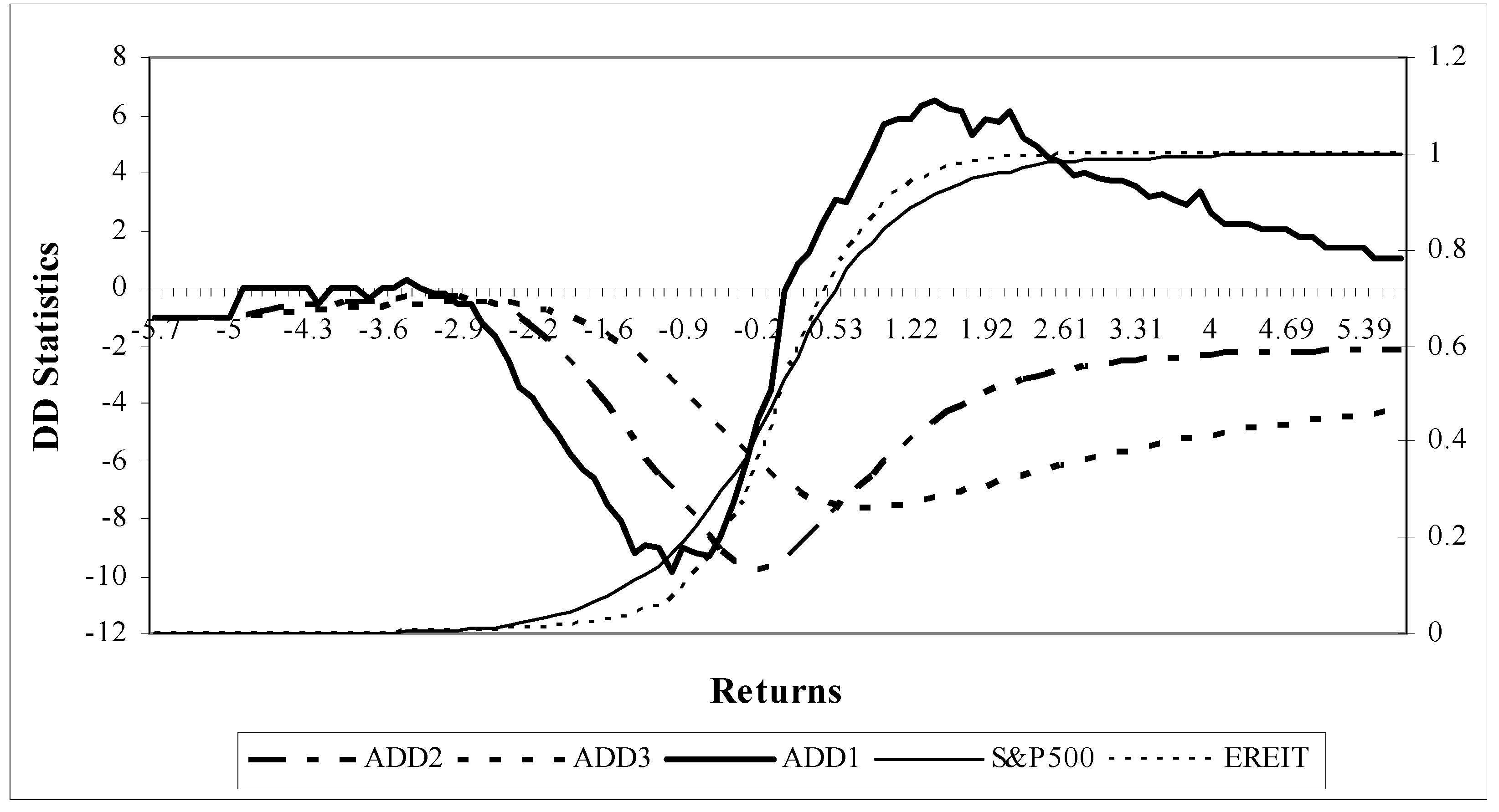
As shown in Table 1, the highly significant Jarque-Bera statistics suggest that the return distributions for all assets are non-normal. The evidence further indicates that all assets have significant skewness and kurtosis. REITs exhibit negative skewness, and mortgage REITs have a very high kurtosis (59.22). The exhibition of significant skewness and kurtosis further supports the non-normality of return distributions. Moreover, on the basis of the findings using the MV criterion, we cannot conclude whether investors’ preferences between assets will lead to an increase in wealth or, in the case of risk-averse or risk-seeking individuals, whether their preferences will increase their expected utility. However, the SD approach allows us to address the issue. 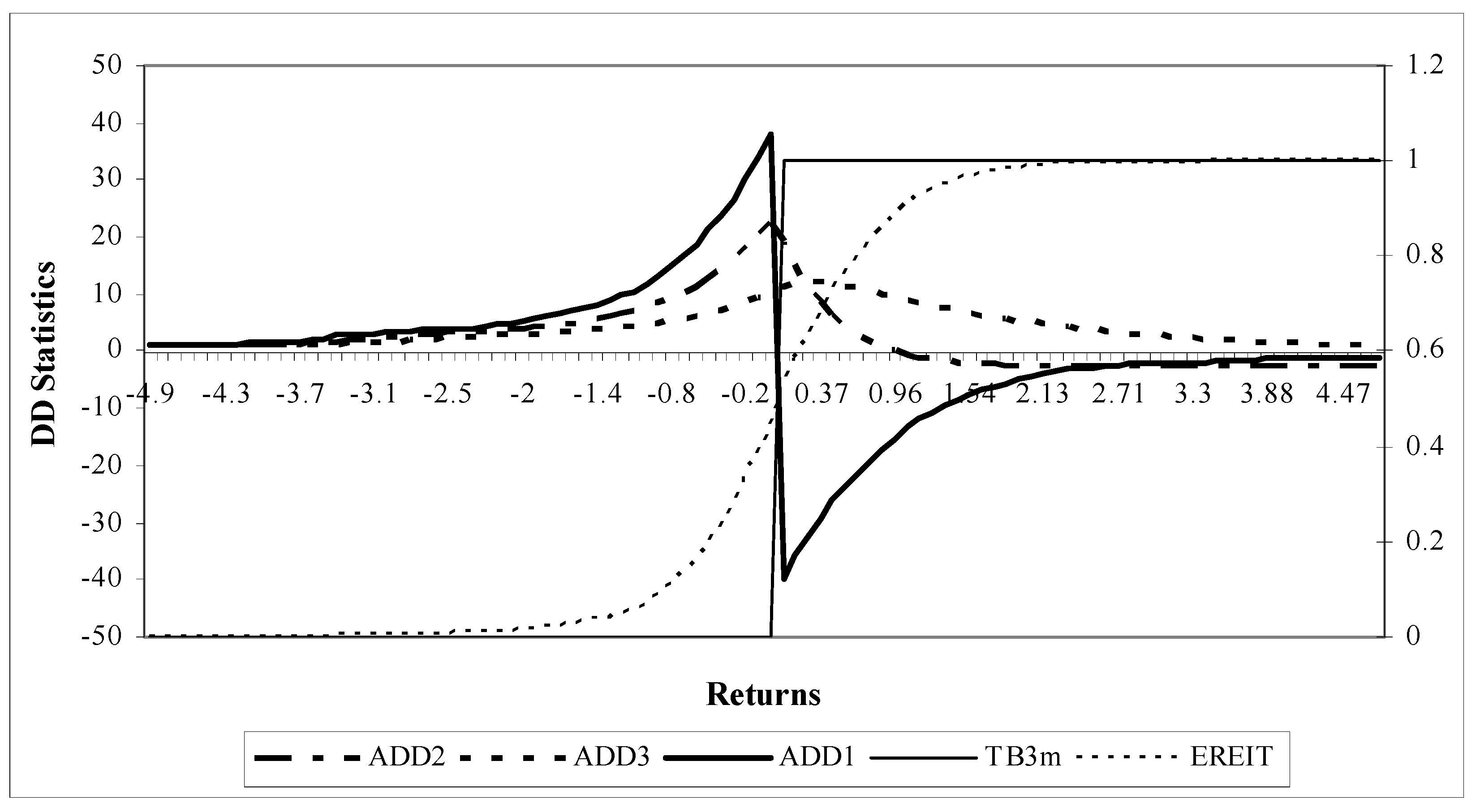To demonstrate the use of the SD approach, we first plot the cumulative distribution functions of returns on equity REITs and the S&P 500 in Figure 1 and plot the CDFs of returns on equity REITs and the 3-month Treasury bill in Figure 2 as examples. The plots show that there is no FASD between any two pairs of returns as their CDFs cross.7

Insert Fig 1 & Fig 2

Figure 1 also shows the ascending DD statistics, $T_j^A$ (j = 1, 2, 3), over the entire distribution of returns for equity REITs and the S&P 500. This figure provides a visual representation of the DD test results. In particular, $T_1^A$ moves from negative to positive along the distribution of returns. This implies that equity REITs dominate the S&P 500 in the downside risk (negative returns), while the S&P 500 dominates equity REITs in the upside profit (positive returns). To compare equity REITs with the 3-month Treasury bill, in Figure 2 we plot the ascending DD statistics for these two asset returns. The DD statistics show different movements from those in Figure 1. We find that equity REITs are dominated by the 3-month Treasury bill in the downside risk and the dominance order reverses in the upside profit.

However, the DD statistics could be significant or insignificant based on the critical values of SMM distributions. The rule set by the DD test states that the null hypothesis can be rejected if any of the t-statistics defined in (4) (or (5)) are significantly different from zero. To minimize the type II error of dominance and to accommodate the effect of almost SD (Leshno and Levy, 2002), we use a conservative 5% cut-off point for the proportion of t-statistics for statistical inference. Using a 5% cut-off point as a benchmark, for the risk-averse, if REITs dominate any of the other assets, we should find at least 5% significantly negative j-order ascending DD statistics, $T_j^A$, and no significantly positive $T_j^A$ statistics. The reverse holds if REITs are dominated by any of the other assets. On the other hand, for risk-seekers, if REITs dominate any of the other assets, we should find at least 5% significantly positive j-order descending DD statistics, $T_j^D$, and no significantly negative $T_j^D$ statistics. The reverse holds if REITs are dominated by any of the other assets.

Insert

Table 2. Results of DD Test for Risk-Averters (1999–2005)

	FASD				SASD				TASD
	% DD>0	% DD>CV	% DD<0	% DD<CV	% DD>0	% DD>CV	% DD<0	% DD<CV	% DD>0	% DD>CV	% DD<0	% DD<CV
ART - DJI	53	18	47	18	0	0	100	27	0	100	100	59
ART - NAS	59	27	41	23	0	0	100	32	0	100	100	74
ART - SP5	49	27	51	20	0	0	100	34	0	100	100	58
ART - TB10	53	30	47	23	63	33	37	0	100	48	0	0
ART - TB3	53	30	47	23	63	33	37	0	100	46	0	0
ERT - DJI	52	17	48	17	0	0	100	27	0	0	100	59
ERT - NAS	59	27	41	23	0	0	100	33	0	0	100	74
ERT - SP5	49	24	51	21	0	0	100	34	0	0	100	58
ERT - TB10	52	32	48	23	62	34	38	0	100	50	0	0
ERT - TB3	52	32	48	23	61	34	39	0	100	48	0	0
MRT - DJI	38	4	62	3	42	4	58	0	57	1	43	0
MRT - NAS	47	13	53	10	29	1	71	12	35	1	65	19
MRT - SP5	43	5	57	3	41	3	59	0	52	1	48	0
MRT - TB10	41	12	59	10	46	11	54	0	92	15	8	0
MRT - TB3	41	12	59	10	45	11	55	0	87	15	13	0
DRE - DJI	54	9	46	15	0	0	100	20	0	0	100	28
DRE - NAS	59	28	41	22	0	0	100	30	0	0	100	64
DRE - SP5	54	21	46	18	2	0	98	25	1	0	99	45
DRE - TB10	53	31	47	26	69	35	31	0	100	62	0	0
DRE - TB3	53	31	47	26	67	35	33	0	100	59	0	0

Notes: The table reports the percentages of positive and negative DD statistics, $T_j^A$ (see eqn (4) for j = 1, 2, 3) for risk-averters, and their significant portions at the 5% significance level, based on the asymptotic critical value of 3.254 of the studentized maximum modulus (SMM) distribution. ERT is equity REIT, MRT is mortgage REIT, and DRE is US-DS Real Estate.ART - DJI means pairwise comparison of all REITs with the Dow Jones Industrial index. Other pairs are defined accordingly.

Table 2 shows the results of the DD test for risk-averters for the entire period. There are four groups showing a pairwise comparison between four types of REITs and other assets.8 We take the pair of equity REITs and the S&P 500 as examples. The evidence from Table 2 suggests that 21% of $T_1^A$ is significantly negative, and 24% of $T_1^A$ is significantly positive for the risk-averse. This implies no FASD between the pair of equity REITs and the S&P 500. We find similar results for all the other pairs, such as equity REITs and Dow Jones Industrials and equity REITs and the NASDAQ.

All $T_2^A$ and $T_3^A$ for the comparison of equity REITs and the S&P 500 are negative along the distribution of returns as shown in Figure 1. In addition, Table 2 shows that 34% of $T_2^A$ and 58% of $T_3^A$ are found to be significantly negative at the 5% level. Thus, we conclude that equity REITs dominate the S&P 500 at second and third order under ASD, implying that any risk-averse investor would prefer equity REITs to the S&P 500 for maximizing utility. On the other hand, for the comparison of equity REITs and the 3-month Treasury bill (and 10-year Treasury note), we find that 23% of $T_1^A$ is significantly negative and 32% of $T_1^A$ is significantly positive for risk-averters. Further inspecting the DD statistics for the second and third order for risk-averters, we see that the 3-month Treasury bill (10-year Treasury note) dominates equity REITs, since 34% of $T_2^A$ and 48% (50%) of $T_3^A$ are found to be significantly positive at the 5% level.

Overall, evidence derived from ascending DD statistics indicates there is no FASD between REITs and other assets, suggesting that investors cannot increase their wealth by switching from one asset to the other and there is no arbitrage opportunity between them (Bawa, 1978; Jarrow, 1986). These results are also evidence that we cannot reject market efficiency. However, by considering the statistics from SASD and TASD, we can determine whether investors could increase their expected utility by switching from one asset to another. In our research, it is apparent that risk-averters prefer REITs (except mortgage REITs) to stocks, while they prefer Treasury constant maturities over REITs for maximizing their expected utility. This implies that they will increase their expected utility by switching their investments from stocks to real estate and from real estate to fixed-income assets.

Insert Fig 3 & Fig 4

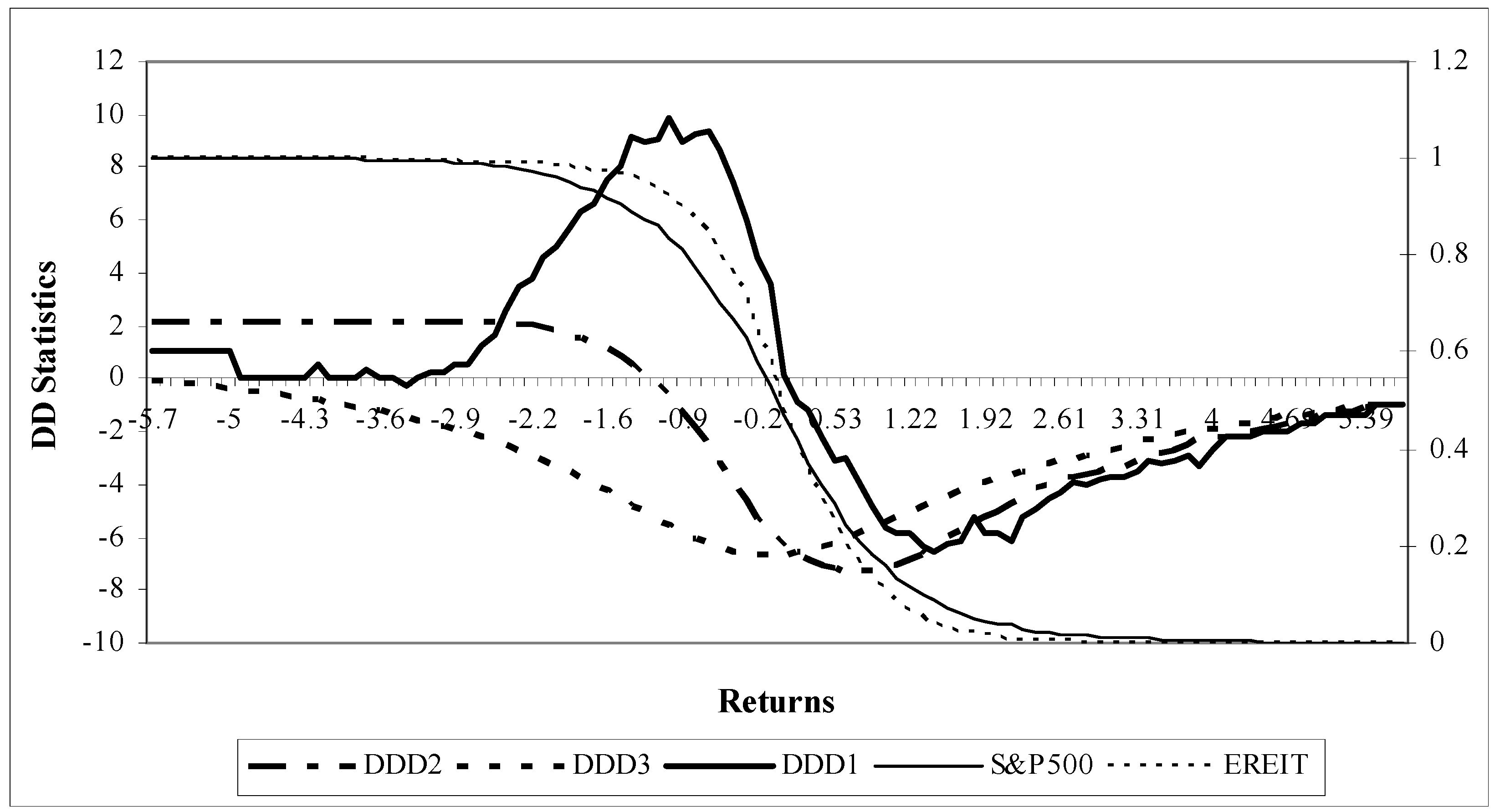
Figure 3 and Figure 4 present the cases for the descending CDF and the corresponding descending DD statistics for equity REITs and the S&P 500 and equity REITs and the 3-month Treasury bill, respectively. Specifically, Figure 3 reveals that the $T_1^D$ is negative in the upside return region and positive in the downside return region, revealing that the S&P 500 is preferred to equity REITs in the upper range of returns and vice versa.

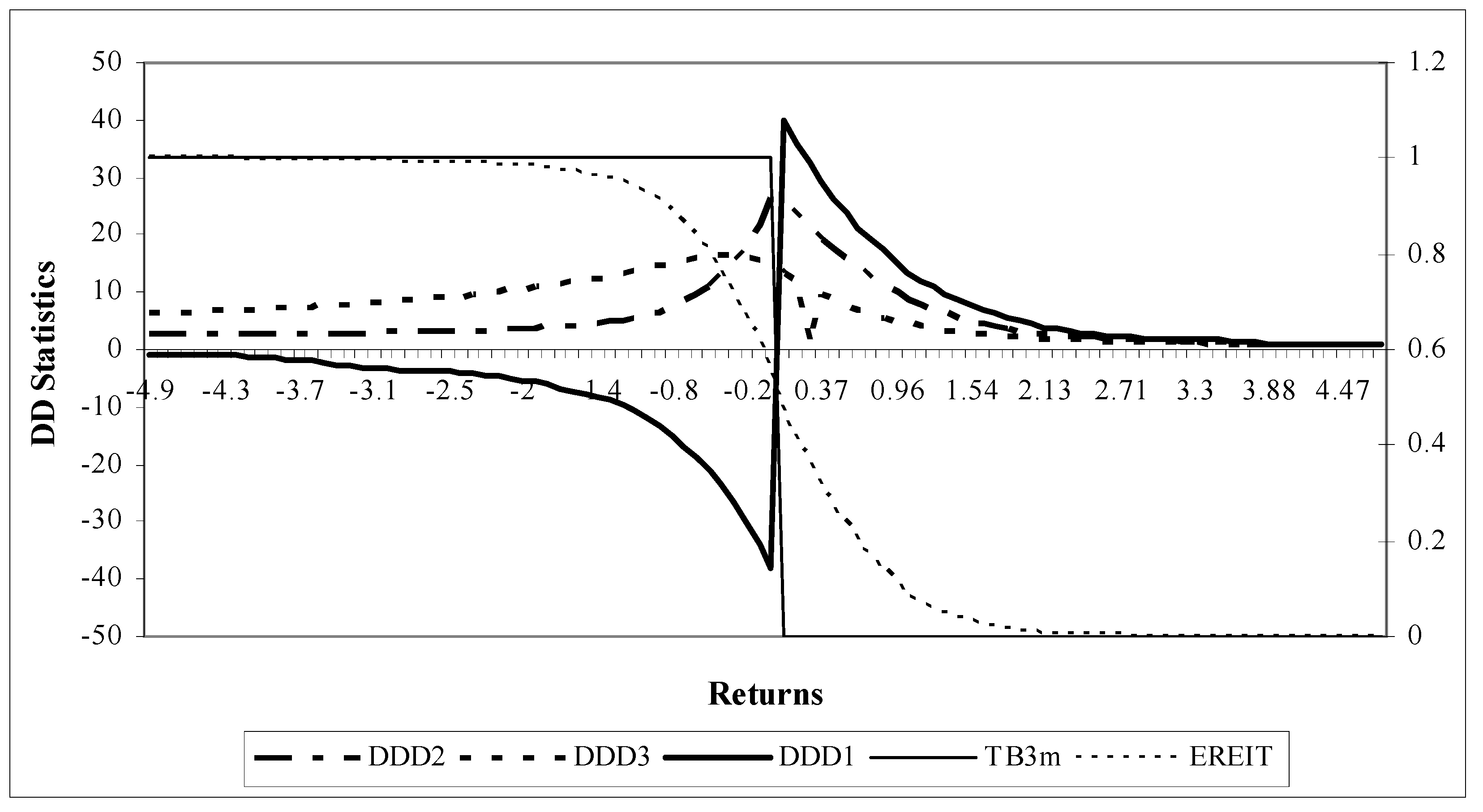
On the other hand, Figure 4 shows the descending CDF and the corresponding descending DD statistics for equity REITs and the 3-month Treasury bill, respectively. Figure 4 reveals that the $T_1^D$ is negative in the downside return region and positive in the upside return region. Putting the information together, it is clear that the 3-month Treasury bill is preferred to equity REITs in the lower range of returns and the reverse is true in the upper range based on FDSD.

Insert

Table 3. Results of DD Test for Risk-Seekers (1999–2005)

	FDSD				SDSD				TDSD
	% DD>0	% DD>CV	% DD<0	% DD<CV	% DD>0	% DD>CV	% DD<0	% DD<CV	% DD>0	% DD>CV	% DD<0	% DD<CV
ART - DJI	41	18	59	18	38	0	62	25	0	0	100	31
ART - NAS	41	23	59	27	27	0	73	30	0	0	100	47
ART - SP5	39	20	61	27	41	0	59	33	0	0	100	41
ART - TB10	47	23	53	30	100	40	0	0	100	67	0	0
ART - TB3	47	23	53	30	100	44	0	0	100	67	0	0
ERT - DJI	44	17	56	17	39	0	61	24	1	0	99	29
ERT - NAS	41	24	59	27	27	0	73	30	0	0	100	47
ERT - SP5	39	21	61	24	41	0	59	33	0	0	100	39
ERT - TB10	48	23	52	32	100	41	0	0	100	66	0	0
ERT - TB3	48	23	52	32	100	45	0	0	100	66	0	0
MRT - DJI	62	3	38	4	100	3	0	0	100	0	0	0
MRT - NAS	41	10	59	13	76	0	24	10	51	0	49	3
MRT - SP5	56	3	44	5	100	1	0	0	100	0	0	0
MRT - TB10	59	10	41	12	100	11	0	0	100	33	0	0
MRT - TB3	59	10	41	12	100	12	0	0	100	36	0	0
DRE - DJI	38	15	62	9	35	0	65	20	0	0	100	24
DRE - NAS	35	18	65	21	38	0	62	28	0	0	100	34
DRE - SP5	47	26	53	31	38	0	62	28	0	0	100	34
DRE - TB10	47	26	53	31	100	33	0	0	100	68	0	0
DRE - TB3	47	26	53	31	100	34	0	0	100	68	0	0

Notes: The table reports the percentages of positive and negative DD statistics, $T_j^D$ (see eqn (7) for j = 1, 2, 3) for risk-seekers and their significant portions at the 5% significance level, based on the asymptotic critical value of 3.254 of the studentized maximum modulus (SMM) distribution. ERT is equity REIT, MRT is mortgage REIT, and DRE is US-DS Real Estate.ART - DJI means pairwise comparison of all REITs with the Dow Jones Industrial index. Other pairs are defined accordingly.

Table 3 reports the descending DD statistics for risk-seekers. As in Table 2, taking the comparison of equity REITs and the S&P 500 as an example, we find that 33% of $T_2^D$ and 39% of $T_3^D$ are negative and statistically significant, respectively. Hence, risk-seeking investors will unambiguously prefer the S&P 500 to equity REITs to maximize their expected utility. On the other hand, if we compare equity REITs and the 3-month Treasury bill, risk-seeking investors will prefer equity REITs to the 3-month Treasury bill as is evident from the fact that 45% of $T_2^D$ and 66% of $T_3^D$ are positive and statistically significant, respectively. Different from the evidence for risk-averters, evidence from second- and third-order $T_j^D$ statistics reveals that risk-seekers will increase their expected utility by switching from real estate to stocks and from fixed-income assets to real estate.

Is there time-varying behavior for risk-averters and risk-seekers? Dynamic asset price movements suggest that asset returns are subject to ongoing external shocks in addition to some big events and extraordinary economic/social disturbances. It is of interest to examine whether investors’ behavior is influenced by the up and down market trend. To address this issue, we divided the entire sample into two sub-periods. That is, we treat the period from January 1999 to December 2002 as an up market and January 2003 to December 2005 as a down market. This allows us to investigate the behavioral differential conditioned on the financial economic environment.

Insert

Table 4. Results of DD Test for Sub-periods

Sub-period 1 (1999 – 2002)		Sub-period 2 (2003 - 2005)
Risk-Averters	Risk-Seekers	Risk-Averters	Risk-Seekers
ART≻2DJI	ART≺2DJI	ART$\cancel{\succ }$DJI	ART≻2DJI
ART≻2NAS	ART≺2NAS	ART$\cancel{\succ }$NAS	ART≺2NAS
ART≻2SP5	ART≺2SP5	ART$\cancel{\succ }$SP5	ART≻2SP5
ART≺2TB10	ART≻2TB10	ART≺2TB10	ART≻2TB10
ART≺2TB3	ART≻2TB3	ART≺2TB3	ART≻2TB3
ERT≻2DJI	ERT≺2DJI	ERT$\cancel{\succ }$DJI	ERT≻2DJI
ERT≻2NAS	ERT≺2NAS	ERT$\cancel{\succ }$NAS	ERT≺2NAS
ERT≻2SP5	ERT≺2SP5	ERT$\cancel{\succ }$SP5	ERT≻2SP5
ERT≺2TB10	ERT≻2TB10	ERT≺2TB10	ERT≻2TB10
ERT≺2TB3	ERT≻2TB3	ERT≺2TB3	ERT≻2TB3
MRT$\cancel{\succ }$DJI	MRT$\cancel{\succ }$DJI	MRT≺2DJI	MRT≻2DJI
MRT≻2NAS	MRT≺2NAS	MRT$\cancel{\succ }$NAS	MRT$\cancel{\succ }$NAS
MRT$\cancel{\succ }$SP5	MRT$\cancel{\succ }$SP5	MRT≺2SP5	MRT≻2SP5
MRT≺2TB10	MRT≻2TB10	MRT≺2TB10	MRT≻2TB10
MRT≺2TB3	MRT≻2TB3	MRT≺2TB3	MRT≻2TB3
DRE≻2DJI	DRE≺2DJI	DRE$\cancel{\succ }$DJI	DRE≻2DJI
DRE≻2NAS	DRE≺2NAS	DRE$\cancel{\succ }$NAS	DRE≺2NAS
DRE≻2SP5	DRE≺2SP5	DRE$\cancel{\succ }$SP5	DRE≻2SP5
DRE≺2TB10	DRE≻2TB10	DRE≺2TB10	DRE≻2TB10
DRE≺2TB3	DRE≻2TB3	DRE≺2TB3	DRE≻2TB3

Notes: $Y{\succ }_j\left({\prec }_j\right)Z$ means Y dominates (is dominated by) Z under order-j ASD (refer to (2)) and $Y{\succ }^j\left({\prec }^j\right)Z$ means Y dominates (is dominated by) Z under order-j DSD (refer to (3)) respectively for j = 1, 2 and 3. Y $\cancel{\succ }$ Z means no SD between Y and Z (refer to (5)).

The results for the two sub-periods are presented in Table 4. As we reported earlier, there is no FSD among all assets studied in this paper for each sub-period, implying that an arbitrage opportunity does not exist among these assets in both bull and bear markets. On the other hand, REITs are found to be dominated by Treasury constant maturities under ASD, while REITs dominate Treasury constant maturities under DSD in both sub-periods, indicating that investors’ behavior concerning fixed-income assets are not influenced by economic conditions. Nevertheless, we observe substantial differences among the distributions of other assets during different time periods. For instance, except for mortgage REITs, all other REITs are found to dominate stock indices under ASD in sub-period 1 but not in sub-period 2. For DSD, we find a change in direction of preference from sub-period 1 to sub-period 2. In particular, the S&P 500 dominates equity REITs in sub-period 1; however, it is dominated by equity REITs in sub-period 2 under DSD, implying that investors’ behavior concerning stocks could be time-varying and influenced by market conditions.

5. Conclusion

It is a widely accepted stylized fact that returns on most financial assets exhibit leptokurtosis and sometimes asymmetry and they are not normally distributed (Peiró, 1999; Patton, 2004; Brooks, et al., 2005). The parametric analysis derived from the MV approach is likely to be misleading or of limited value. In addition, empirical findings using the MV approach cannot be used to decide whether investors’ portfolio preferences will increase wealth or, in the case of risk-averse investors, lead to an increase in utility without an increase in wealth. Given the limitation of the MV approach and the lack of a clear solution to the fat-tail distributions, this study is based on the SD approach, which is not distribution-dependent, and can shed light on the utility and wealth implications of portfolio preferences by exploiting information obtained from higher order moments to test their performance.

By investigating the data on REITs and five other assets over the entire sample period of 1999–2005, we find that all REITs (except mortgage REITs) dominate the three stock indices but not the Treasury constant maturities using the MV criterion. We also find no FSD between them. This implies that investors cannot increase their wealth by switching from one asset to another. However, REITs (except mortgage REITs) stochastically dominate returns on the three stock indices but are stochastically dominated by fixed-income securities, the 3-month Treasury bill, and the 10-year Treasury bond at the second and third order for risk-averters. We find the reverse case for risk-seekers. This means that to maximize their expected utility, all risk-averse investors would prefer to invest in real estate than in the stock market, subject to trading costs. However, if we compare real estate to fixed-income assets, they would prefer fixed-income assets to real estate. On the other hand, all risk-seeking investors would prefer to invest in the stock market than in real estate (or in real estate rather than in fixed-income assets) to maximize their expected utility. In addition, we find that investors’ behavior concerning fixed-income assets is not influenced by economic conditions, while their behavior concerning stocks is time-varying and influenced by market conditions.

Last, we note that SD is found to be important in risk measurement, since the first-order SD is found to be equivalent to the value-at-risk, while the second-order SD is found to be equivalent to the conditional value-at-risk (Ogryczak and Ruszczyński, 2002; Leitner, 2005; Ma and Wong, 2006). Thus, adopting SD for analysis will include inferences made by employing VaR and conditional VaR. We also note that if the prospects belong to the same local-scale family, the preference for the prospects drawn from the MV criterion will be the same as that drawn from the ascending SD criterion (Meyer, 1987; Wong and Ma, 2008). In addition, this paper extends the work on the SD test from risk-averters to risk-seekers. Further research could include extending our work to test the SD theory for investors with S-shaped and reverse S-shaped utility functions as developed by Levy and Wiener (1998), Levy and Levy (2004), Wong and Chan (2008), among others.