
Portfolio Optimization and Mortgage Choice


Department of Mathematical Sciences, University of Copenhagen, Universitetsparken 5, DK-2100 Copenhagen, Denmark
*
Author to whom correspondence should be addressed.
J. Risk Financial Manag. 2017, 10(1), 1; https://doi.org/10.3390/jrfm10010001
Submission received: 6 October 2016
/
Revised: 23 December 2016
/
Accepted: 27 December 2016
/
Published: 3 January 2017
(This article belongs to the Section Mathematics and Finance)
Abstract
:This paper studies the optimal mortgage choice of an investor in a simple bond market with a stochastic interest rate and access to term life insurance. The study is based on advances in stochastic control theory, which provides analytical solutions to portfolio problems with a stochastic interest rate. We derive the optimal portfolio of a mortgagor in a simple framework and formulate stylized versions of mortgage products offered in the market today. This allows us to analyze the optimal investment strategy in terms of optimal mortgage choice. We conclude that certain extreme investors optimally choose either a traditional fixed rate mortgage or an adjustable rate mortgage, while investors with moderate risk aversion and income prefer a mix of the two. By matching specific investor characteristics to existing mortgage products, our study provides a better understanding of the complex and yet restricted mortgage choice faced by many household investors. In addition, the simple analytical framework enables a detailed analysis of how changes to market, income and preference parameters affect the optimal mortgage choice.
1. Introduction
This paper studies optimal investment and consumption in relation to mortgage choice as viewed from the perspective of a household investor. In a financial market consisting of a bond and a money account, we formulate stylized versions of the two most common mortgage products found in the market today. Next, we formulate and solve a simple investment consumption problem of an investor who seeks to maximize the utility of consumption during a finite term of optimization. The investor has an uncertain lifetime, a fixed housing position, a labor income and initial mortgage debt funded in the bond market. In addition, we assume that the investor is constrained to have zero financial debt upon time of death or termination, whichever occurs first. As a consequence, the house price risk is fully absorbed in consumption after the term of optimization and housing wealth is disregarded in the optimization problem. The assumed income is perfectly correlated with the bond, and the financial market related to the investment problem is thus complete. The simple setup provides a benchmark for the isolated mortgage decision of a household and allows us to express the optimal investment strategy of the investor in terms of optimal mortgage choice.
Disregarding the housing decision means that we enter the financing decision after the housing decision has been made and that the time horizon of our decision problem is before changes in the house prices are absorbed in consumption. We emphasize here that we think that this is a realistic situation in many mortgage decisions from a practical point of view. Additionally, in any case, we believe that it deserves to stand alone as an extreme, yet relevant, benchmark in sharp contrast to the standard formulation, where changes in house prices are continuously absorbed in both housing consumption and consumption of other goods.
By translating the abstract optimal bond position of our investment problem into positions in the stylized marketed mortgage products, we derive the optimal mortgage choice, which can be used directly in practical advice. Furthermore, it enables us to show that full positions in the stylized mortgage products match particular (extreme) customer characteristics. This is a novel insight that we have not encountered in existing literature. It is valuable to characterize the income and preference profiles of individuals who optimally choose these full positions, since many homeowners in practice hold full mortgage positions of this type. Thus, our representation of the optimal bond portfolio in terms of mortgage product choice combined with our derivation of the characteristics of investors with full positions in particular mortgage products is innovative, practically relevant and adds value to the existing line of literature. We bridge a gap in the literature between the closed-form solutions of portfolio problems with a stochastic interest rate (see, e.g., [1,2,3,4]) and the mortgage choice literature, which is dominated by numerical studies (e.g., [5,6,7]). Numerical studies in general allow for more realistic market settings, but hinder analytical conclusions on how the parameters directly affect the optimal portfolio mix, whereas closed-form solutions enable a more detailed study of the optimal portfolio composition and optimal repayment of a mortgage at the cost of realism. In particular, the analytical solutions in this study reveal how stylized versions of the two most common products in the market today, the Fixed Rate Mortgage (FRM) and the Adjustable Rate Mortgage (ARM), can be framed as the optimal choice of two extreme investors. In addition to this, the analytical framework provides suggestions to how a moderate investor should fund a mortgage as a mixed portfolio of the two.
With the introduction of human capital, suggesting the value of future labor income to be hedged as if it were a traded asset, Bodie et al. [8] established that inclusion of labor income in the investment problem generally induces negative tangible investments in the risk-free asset. The literature on stochastic control theory has since developed to provide closed-form solutions to investment problems with stochastic interest (see [3] and the references therein). In Kraft and Munk [4], such an asset allocation problem with a stochastic interest rate is solved analytically under the assumption that labor income and housing can be perfectly hedged in the market and by allowing allocation in housing to be continuous in time. The resulting strategy in Kraft and Munk [4] also includes a large negative position in the risk-free asset, and they, as well as Bodie et al. [8] swiftly interpret this negative position as a mortgage. In contrast, the strand of mortgage choice literature (see particularly [5] and the references therein) often studies particular mortgage products, seeks to capture more realistic (incomplete) market settings, includes complex borrowing constraints and discrete actions, such as prepayment and default, and hence, requires numerical solutions. The downfall of these studies is that they can only evaluate the performance and optimality of the products in the specific market setting and preferences chosen for the study, but do not immediately provide insight to the mixed effects of market and preference parameters and their influence on the optimal portfolio mix and repayments over time.
In Campbell and Cocco [5], the maximum utility is determined for households with three distinct mortgage products in a detailed and realistic market setting. In Van Hemert [6], the optimal mortgage choice is derived as an aspect of the overall household asset allocation problem, including housing. Kraft and Munk [4] differ substantially from the numerical studies of Van Hemert [6] and Campbell and Cocco [5] by solving the investment problem analytically in a continuous-time setup, but apart from this, all three studies see the decision of optimal mortgage funding as part of a total asset allocation problem, including a housing position, as well as optimal investment in stocks. All three studies reach a clear consensus towards the ARM predominantly being the optimal mortgage for a household investor. There is a discrepancy between these results and the mixed practices of the general population, where in Denmark, as an example, a large proportion of mortgagors chooses FRMs as opposed to the risk-free asset. In 2013, over 30% of Danish mortgages were FRMs (see [9]), and in Badarinza et al. [10], it is reported that the 30-year FRM is the dominant choice in the U.S. This study is motivated by this discrepancy, and we wish to determine the characteristics of a mortgagor who optimally chooses an FRM in contrast to the predictions of the aforementioned studies. Recent significant changes in the Danish mortgage market have led to a greater variety of products, including the introduction of adjustable rate mortgages and interest-only mortgages (see [11,12], for an introduction to the Danish mortgage system), and the new products accentuate the complexity of the financial decisions faced by household investors and encourage research on what defines a good mortgage product. We seek to contribute to this discussion by capturing the characteristics of the mortgagor who optimally chooses the two most common contracts offered in the market today, hereby providing an outset for the development of new and better product designs.
The focus of the study can be summed up in the following questions: (1) Is it within a simple setup possible to mathematically formulate investment problems, to which existing mortgage products in the market today are the optimal solution? Additionally, (2) does the general structure of the solutions to this type of problem provide insights to the optimal mortgage choice of a broader class of households?
The study includes uncertain lifetime of the investor, following the work of, e.g., Yaari [13] and Richard [14], and is otherwise kept in a very simple continuous-time setting with a stochastic interest rate and investment in term life insurance, a bond and a bank account. In the first part of the study, the main characteristics of two loan products obtainable in the Danish mortgage market are formalized in a simple setting. This enables a comparison between real-life mortgage products and the theoretical results within stochastic control theory. In the second part of the study, a life cycle investment problem, similar to Kraft and Munk [4] with the addition of uncertain lifetime, is solved analytically in a market with a Vasicek interest rate and power utility preferences. Finally, direct links between the stylized mortgage products and the preferences of special cases of the power utility investor are established. More generally, basic relations between utility preferences, assumptions of labor income, mortality and the optimal mortgage choice for a household investor are discussed.
One might be able to match optimal investment strategies to existing mortgage products in a richer setup, including, e.g., investments in other assets and housing, utility of pension savings (other than the fixed housing position), a prepayment option on the FRM at par, considerations of the mobility of mortgagors, inflation and a richer specification of the labor income. However, our setup provides a simple benchmark where significant relations regarding optimal mortgage choice are captured, specifically providing an initial intuition behind the choice of FRMs.
2. The Market Model
The financial market is assumed to be a complete bond market specified through investment in a bond and a bank account. The P-dynamics of the interest rate are assumed to be Vasicek modeled,
By arbitrage arguments, the market value of a Zero Coupon Bond (ZCB) with maturity T follows the dynamics:
with and denoting the market price of risk. In this paper, it is assumed that the market price of risk is constant, , and the Q-dynamics of the interest rate are then given by:
The rolling bond with maturity constantly years into the future, (and thereby, constant volatility ), is chosen as exogenously given, to complete the market, giving the investment opportunities:
Any other bond can now be hedged through investment in the bank account and the bond .
In the following sections, we formulate an isolated mortgage choice investment problem, which excludes optimization of investments in other assets, such as stocks, Real Estate Investment Trusts (REITs) and houses (included in, e.g., Kraft and Munk [4]). This does not restrict an underlying correlation between the bond and other assets. However, since the investment problem we formulate and answer in the following section is only concerned with investments in the bond and money account, we do not introduce the other assets.
In addition, the investor is assumed to have uncertain lifetime with mortality rate and access to a term life insurance market that is priced actuarially fair and without profits. Expressed through term insurance paid out upon death, this means that the price at a given time t to be covered instantaneously for the amount x is .
While alive, the investor receives a labor income at rate perfectly correlated with the bond, by the P-dynamics:
With this specification, the income rate may increase with a constant and/or proportionally with the short rate. In addition, the income is perfectly correlated with the bond through . As a result, the income can be perfectly hedged by the investment opportunities offered in the optimization problem. With this simple problem formulation, it is meaningful to interpret the income simply as the household budget available for mortgage payments or as the rudimentary income predictions used in current mortgage advice.
The human capital of the investor is uniquely determined by the market value of the future labor income. In the case including mortality, the market value corresponds to the discounted payment stream under the risk-neutral measure Q (by mortality and interest),
for a given deterministic function , which is derived later. It is here noted that with perfect correlation, the labor income can be treated as if it were a traded asset, as suggested by Bodie et al. [8].
2.1. Realism and Limitations
In this study, the purchase of a house is an investment fixed at time 0. The house investment is not changed during the term of optimization we consider. Furthermore, the capital gains from the house investment can at a future time be reflected in consumption, but not during the term of optimization we consider. If one thinks of the term of the optimization as the retirement age, the house represents an investment for retirement consumption. At retirement, capital gains can be realized by either selling the house or borrowing with the house as collateral. Probably, for many homeowners, the decision about which house to buy reflects in practice this long-term perspective. Since we assume that the housing decision is fixed at time 0 and since changes in the house prices are assumed to be irrelevant for our period of optimization, we have technically separated the financing decision away from the housing decision.
The two-step decision making process reflects the homeowner who buys a house (chosen from, e.g., a savings perspective or affordability) and who then seeks a financing construction without taking house price movements into account as a source of consumption in the borrowing period. Until retirement, the financing of the loan and the income are the main sources of consumption. After retirement, when loans are repaid, the income is lost, and retirement consumption is financed by the house price (selling or borrowing) together with any other savings. In this study, we assume that the housing decision is already made and focus, exclusively, on the financing decision. In other studies, the house is viewed as an asset taking part in the portfolio optimization, and utility is measured from housing (see Grossman and Laroque [15]), as well as non-housing goods (see, e.g., Damgaard et al. [16], Flavin and Nakagawa [17] and Corradin et al. [18]). House price movements are immediately (rather than after retirement only), and sometimes continuously, integrated into consumption. In Kraft and Munk [4], even the housing decision is rebalanced continuously by, e.g., up- or down-grading the house size as part of the portfolio. Probably, for most household investors, the appropriate portfolio model lies somewhere in between our simple two-step approach and the integrated approach of, e.g., [4]. In any case, we find much value in understanding the solution to our (extreme) simple model as a benchmark. By excluding housing wealth in our optimization problem, we derive the optimal mortgage choice of an investor that does not continuously speculate in future house price movements. As a result, the investment strategy is not sensitive to the modeling of house prices. In particular, with the separated financing decision, we are able to identify (theoretical) investors to which existing mortgage products are the optimal choice.
As mentioned in the Introduction, portfolio problems, including labor income, are known to result in large negative positions in the risk-free asset, even when not including housing investments. Large negative positions of individual households are not realistic in the real world, unless the money is invested in a durable good (such as a house). No bank will lend a young person one million DKK solely on the basis of expected future income. The only possibility young people have for such a loan is to purchase a house. Although the house is considered a consumption-good in this present paper, our setup is still indirectly assuming that the house functions as a collateral for the bank, such that there is negligible credit risk involved in the mortgage contract and such that mortgage contracts are offered on market conditions independent of the characteristics of the particular individual household. Danish homeowners are only allowed to fund a maximum of 80% of their house purchase with a mortgage bond. In addition to this, the Danish mortgage market is based on pass-through securities, by which there are only administrative costs in addition to the market price of interest risk and diminishing credit risk (see [12]). This is in contrast to many other countries where mortgages carry an additional loading, which reflects the credit risk of the individual consumer. In Denmark, all customers who are assessed to be eligible to take out a mortgage of a certain size (hereby avoiding the worst credit risks) will be offered the exact same market-based mortgage rates, irrespective of income and mortgage size. By the pass-through system, the pure bond market prices are thus very close to what the customers actually pay (in Denmark), and in this sense, a very simple model including only a bond and a bank account fairly accurately captures the portfolio choice a customer faces when choosing the right mortgage.
As concluded by, e.g., Baesel and Biger [19], Statman [20] and Campbell and Cocco [5], inflation risk is an important factor in the optimal mortgage choice, but since our main focus is to capture the two common products in the market that are not inflation indexed, this aspect is left out in our model. However, we briefly comment on how an inclusion of inflation might affect the results later on.
3. Stylized Mortgage Products
With a root in historic regulation, most mortgage products in Denmark today are communicated and constructed through specification of an interest rate, by which the principal and payments are uniquely determined. This interest rate can be fixed over a long period of time or regularly adjusted, but either way, the construction of the payments of the loan is overall the same. This is in contrast to the U.S. mortgage market, where a wider variety of repayment profiles are offered, see, e.g., Alm and Follain [21] for a description of three alternative repayment profiles in the U.S. In the following sections, we first describe the general structure of these interest rate profile mortgages and then continue to specify special cases considered to represent stylized versions of a typical FRM and ARM.
3.1. A General Interest Rate Profile Design: The Fn-Loan
The Fn-loan is a type of adjustable rate mortgage, where the adjustable interest rate and total payment stream are determined every n-th year. The interest rate is determined by the market prices every n-th year, such that the interest rate and payment stream are constant in the i-th period between the so-called refinancing of the loan. For the Fn-loan with maturity T, let , and let denote the refinancing nodes for . Furthermore, let . For any , the principal follows the piecewise deterministic dynamics:
for every and where is determined in the beginning of the previous refinancing period and:
where denotes the annuity factor from time to T with constant interest . With this construction, the principal is at any time given by:
The interest of the Fn-loan is determined at each of the N nodes on the basis of the annuity bond with maturity at the next refinancing node along with a ZCB to ensure that the remaining principal is consistent with the constant interest at next refinancing. By this, the market value and the principal of the loan do not equal in the period between the refinancing nodes. At every refinancing node , the Fn-loan is characterized by the constant interest rate , which is at all nodes determined through an annuity bond with termination at the next refinancing node, , and similarly, the price of a ZCB, , so as to satisfy:
In other words, at every refinancing node, it is left to determine the interest rate for which:
The interest rate , solving this problem, is unique under the constraint , and the solution can be found numerically.
3.2. The Fixed Rate Mortgage
In the special case where , the Fn-loan corresponds to a basic FRM, as there is no refinancing before maturity T, hereby achieving the constant payment stream of a usual FRM. The market value of an FRM initiated at time 0, with maturity T and initial principal , will at all times be proportionate to the annuity bond by:
By this definition, the fixed rate mortgage can be hedged in the complete bond market specified above. It is noted that in the simple setting, the fixed interest on an FRM with a certain maturity is unique. The simple FRM presented in this section can be repaid prematurely by the market-value of the constant payment stream, but not at principal value. In reality, the usual long-term FRMs in Denmark, as well as the U.S., have a prepayment option at par, and through this, several FRMs might be available with the same maturity, but different fixed interest rates, achieved by differences in their market values (see [7], for an inclusion of the prepayment option). Furthermore, as a result, the inclusion of mobility will not have an impact on the rates, like in the market model of, e.g., Brueckner [22].
In other related literature, the FRM is often not directly specified, but referred to as (any) bond investments. In Van Hemert [6], as an example, the FRM is modeled as a negative position in the 10-year bond, which does not quite capture the features of the bond portfolio needed to construct the constant payment stream traditionally known from an FRM.
3.3. The Adjustable Rate Mortgage
The piecewise structure of the Fn-loan in no case matches the solution to the continuous-time optimization in the following section, so the limit when n tends to zero and N thereby tends to infinity is studied instead. The limit Fn is in the rest of the paper referred to as the ARM.
For simplicity, assume that the maturity is dividable by the number of refinancing nodes, such that for all . Then, , and by Equation (12), the interest rate solves:
When and , the right-hand-side can be written as:
and through L’Hopital’s rule and the analytically known price of the zero coupon bond under the Vasicek model, it is concluded that in the limit, Equation (14) corresponds to:
Thereby, the ARM develops like a bank account with payments continuously calculated by an annuity factor with the short rate of interest, and the dynamics and payments from Equations (8) and (9) become:
Besides, the market value of the loan at all times equals the principal:
This is a direct consequence of the construction of the Fn-loan, as it ensures that the market value and principal are equal at every re-financing (which is now at all times as ). The payments of the loan are at all times given by:
Here, the payment stream is at all times calculated by dividing the current value of the loan with an annuity factor using the current interest rate (as a constant discounting factor). The ARM is commonly modeled as a negative investment in the bank account, without specifying the payment stream, however (see, e.g., [6]).
4. Optimal Investment and Consumption
It is assumed that at time 0, the investor initiates a debt of size . As mentioned previously, this can be viewed as a person buying (consuming) a house at time 0, funded by a mortgage. The investor is assumed to have an income throughout the time horizon. The assumed income does not need to reflect labor income, but can also be viewed as the household’s maximum amount available to spend on mortgage payments; a point that will be discussed in more detail later. It is assumed that the portfolio of the investor is self-financing with income rate given by Equation (6), controlled consumption and term insurance . While alive, the investor’s tangible wealth under the P-measure follows the dynamics:
with expressing the proportion of wealth invested in the rolling bond and the remainder invested in the bank account. The payments of the mortgage are defined to be:
Through this definition, the payments are expressed in positive terms. It is assumed that the mortgage is repaid within the investment horizon T, and through this, it is assumed that the investor has the indirect bequest motive/constraint of leaving a debt-free house in the possession of the heirs at time T.
Considering an investor who is only interested in optimizing consumption, the investor’s value function, while alive, is assumed to be:
where is the random variable indicating whether the investor is alive at time t (being equal to one, and otherwise zero). The investor measures the utility of consumption by a power utility function with risk aversion parameter γ and with a bias towards consumption today through the time-preference parameter δ. The mortality is assumed to be independent of the financial risk, and hence, the random variable is replaced by the, at time t, conditional survival probability, . The traditional problem of optimizing the utility of consumption under the P-measure is now formulated by:
where denotes the set of admissible strategies. We allow for borrowing and short-selling in the investment strategy π. It is assumed that the investor is constrained to be debt free at time of death, and hence, the tangible wealth and insurance are required to be greater than or equal to zero. Hence, the term insurance is at all times required to satisfy . Furthermore, the investor is assumed to be restricted by a borrowing constraint, such that the total wealth of the individual is greater than or equal to zero at all times. The total wealth of the investor is the sum of tangible wealth and the human capital defined in Equation (7). These conditions enable an analytical solution. With the introduction of a stochastic interest rate, the problem involves solving the HJB equation for the three-dimensional state process . With the above market assumptions, the HJB equation is given by:
with boundary condition:
The value function is guessed to be in the form:
where denotes the market value of the labor income specified in Equation (7), and the function g is determined following the arguments in Appendix A. The solution to the investment problem is specified in the following subsection.
4.1. Solution to the Optimal Investment and Consumption Problem
The optimal consumption, investment and term life insurance are given by:
with:
and:
when suppressing some of the dependencies for notational convenience. The derivation of the above results can be found in Appendix A. When , the solution corresponds to a simple case of Kraft and Munk [4]. This conclusion is achieved by equaling retirement age to the end of optimization T, setting the utility of housing consumption to zero, setting the Sharpe ratios of the stock and house dynamics to be zero in the setup of Kraft and Munk [4] and then asking for the optimal investment strategies in this full market. In this case, there is no incentive for the investor to invest in stocks and houses (and REITs), but by construction, this requires the harsh assumption that there is no gain (in expectations) from such risky investments. This is not required in our simpler problem formulation where housing demand is captured by a fixed housing position and the investor optimizes over the funding of this purchase. This is a benchmark problem formulation that, we believe, reflects the mortgage decision of many households.
We immediately observe how the F- and g-function both resemble the price of annuity bonds. The F-function is adjusted to account for the future stochastic labor income expressed by Equation (6), whereas the g-function is adjusted by the subjective preference parameters γ and δ. The subjective adjustment of the g-function corresponds to an adjustment to the preferred consumption pattern (which is not constant like the payment stream of the annuity bond). When the δ parameter is high, consumption now is preferred to consumption later, and thus, the value of the g-function is smaller than that of the annuity bond. For the risk-averse investor, there is little incentive to postpone consumption in trade for future investment gains, and thus, the g-function approaches an annuity-bond for . In addition, both the F- and the g-function are adjusted to account for mortality, since the payment streams of and are expected to terminate prematurely with some probability (unlike the constant payment stream of the annuity bond). Thus, with a high mortality rate, both the F- and g-function are substantially smaller than the price of an annuity-bond.
4.2. Optimal Term Life Insurance
By Equation (29), it is seen how the addition of mortality and term life insurance in the investment problem and the restriction that the tangible wealth cannot be negative at time of death make it optimal for the investor to continuously cover the loan with term life insurance in case of death. We observe that the insurance must at all times cover the market value of the loan, and in the case of an FRM, it is thus not just the remaining principal that is covered, but the stochastic market value as specified in Section 3.2. This corresponds to full coverage by products known in the market as Mortgage Life Insurance (MLI). Although the insurance demand is a direct consequence of the debt constraint, an investment problem like the one above provides a formal framework in which it is optimal to engage in such a contract. The MLI is the only type of contract that captures the risk of not being able to repay the mortgage at its market value in the case of death, and for the investor who wants to leave a mortgage-free house to the heirs in case of death and who optimizes the utility of consumption, the optimal way to cover this risk is through MLI priced actuarially fair. However, Villeneuve [23] reports of very limited competition in the French market of MLI and high prices, and thus, one cannot conclude that the current products offered in the market match the demand suggested in this study.
4.3. Optimal Consumption
It is seen that the total wealth under optimal investment has the dynamics:
thereby forming a self-financing portfolio while alive with consumption and proportion:
invested in the rolling bond, which is equivalent to the optimal investment strategy without labor income. The optimal consumption is at all times:
where the g-function specified in Equations (30)–(32) corresponds to a subjective valuation of a constant payment stream similarly to the market-value of an annuity-bond, but adjusted by the preference parameters γ and δ and accounting for the mortality . The consumption dynamics follow:
and are independent of the current level of mortality. Although the dynamics are independent of mortality, the consumption patterns differ through the difference in starting point, due to a different initial valuation of the total wealth in the F-function through Equation (35) and also the impact of the subjective valuation in the g-function through Equation (32).
5. Comparison between Optimization and Stylized Mortgage Products
A number of insights are immediately apparent by the analytical solutions. First, it is recognized that in the cases where , then the mortgage payments no longer depend on the current level of income. This is concluded by definition in Equation (21) and with optimal consumption as given in Equation (27). The independence of the current level of income is desirable, when trying to match the solution from the optimization problem with standard mortgage products offered in the market today. It is seen that when the parameters fulfil:
and the optimal proportion invested in the rolling bond is given by:
This is recognized to equal the investment proportion of total wealth given in Equation (37), and it is hereby concluded that tangible wealth is a constant proportion of total wealth when . Enforcing the parameters to be related as above is artificial in the general case of an investor; nevertheless, in the extremes of the risk aversion parameter γ, they provide some cases that can be directly linked to products in the market.
5.1. The Investor Who Optimally Chooses the ARM
It is optimal for the log-investor () with , and (e.g., ) to fund the mortgage 1:1 in the bank account, without additional borrowing when . In this particular case, the optimal proportion in Equation (41) becomes . We note that this parameter choice is sufficient, but not necessary for . Given the complexity of the solution, we do not exclude the possibility for other parameter combinations that give . A mortgage funded entirely in the bank account corresponds to the ARM described in the previous section funding wise, and it is concluded that a log-investor with income rate continuously increasing with the short rate (and possibly a constant term equivalent to a preference towards consumption later, ) optimally chooses an ARM. When , the mortgage is funded with a constant negative proportion of total wealth in the rolling bond. When considering an initial negative tangible wealth, this corresponds to a positive investment in the rolling bond and short-selling in the bank to cover the mortgage, as well as the positive investments. The corresponding optimal payments of the mortgage are determined by a fixed-rate annuity proportion:
where the fixed rate is equivalent to the time-preference parameter δ. These payments differ from the repayment profile offered in the market today. The repayment profile for the ARM formalized in Equation (19) in the previous section uses the short rate as the annuity factor and is hereby heavily influenced by the current (diffusive) level of interest. In contrast to this, full investment in the bank account and the repayment profile given by Equation (42) result in smooth payments. With the addition of mortality, the payments become distorted by leaving room for the insurance premium, but the investment is still 1:1 in the bank account. The inclusion of mortality gives a higher initial payment of the mortgage and a lower consumption throughout the duration, as there are no changes to the consumption dynamics.
5.2. The Investor Who Optimally Chooses the FRM
In the case without mortality, , and constant labor income, , it is immediately seen from Equation (21) that . If the investor furthermore has infinite risk aversion, by , then the optimal consumption dynamics in Equation (39) are constant, since . In other words, the optimal consumption and payment of the loan is constant throughout the horizon, and the optimal investment corresponds to an annuity bond, similarly to the result of positive investments in Munk and Sørensen [2]. We note that the parameter choice is sufficient, but not necessary for a constant payment stream. Given the structure of the solution, we find it unlikely, but do not rule out, that there exists other parameter choices that result in a constant payment stream. The negative investment in the annuity bond, can be viewed as the simplest type of FRM, as described in the previous section, and it is concluded that the infinitely risk-averse investor with constant income optimally chooses an FRM. Although the present setup is very simple, the result is in line with the empirical results of Coulibaly and Li [24], who find evidence that more risk averse mortgagors are more likely to choose an FRM.
With mortality included, the functions F and g no longer correspond to the constant annuity bond, but instead to the mortality-adjusted annuity bond. Through this, the investment proportion adjusts slightly to account for the additional premium that needs to be paid at all times and to account for the changes in hedging demand. In total, the changes in the investment strategy are very small, however, and the position still resembles a full investment in the FRM with a small adjustment to account for the predicted insurance premium throughout the duration, hereby leaving room for some hedging through the bank account.
As studies before have shown (e.g., [4]), the assumed labor income has a direct and substantial effect on the optimal investment and consumption strategies. Within the setup of this paper, the labor income hereby directly affects the optimal mortgage choice. It has been demonstrated that in the case where labor income is assumed to behave like an annuity bond, i.e., , then the optimal mortgage is entirely funded by an FRM if the investor at the same time is infinitely risk averse and without mortality risk. Although it is only in the extreme case of the infinitely risk averse investor that it is optimal to maintain an FRM throughout the investment horizon, the absence of alternative mortgage designs in the market today might drive investors with an expected constant level of income towards an FRM, even if not infinitely risk averse.
5.3. A Moderate Investor
In this section, we restrict ourselves to consider only the cases where , corresponding to a differentiable, locally risk-free, but yet stochastic, labor income, and it is seen that the amount invested in the rolling bond can then be represented by three terms:
First is a constant proportion of total wealth corresponding to the speculative demand of a utility optimizing investor. Second is a term relating to the interest rate sensitivity of the human capital through the derivative . Finally, there is a term related to the interest rate sensitivity of the subjective valuation of the future consumption stream through the derivative . The first and last term correspond to positive investments, while the second term corresponds to negative investments for general parameter settings.
The function g expresses the rate of consumption to total wealth in Equation (27), and in the case of the infinitely risk-averse investor, it equals the price of the annuity bond, . Hence, the rate of consumption is in this case determined by how large an annuity payment the total wealth corresponds to. Two things change in the optimal investment when the risk aversion parameter does no longer tend to infinity. First, the constant term arises in Equation (43), accounting for a speculative positive demand in the bond, to obtain the Sharpe ratio . Secondly, the g function is no longer equivalent to the annuity bond, but is distorted to account for the risk aversion parameter γ. It is worth noting that the speculative demand remains strictly positive throughout the investment period, whereas the hedging demands expressed through the F- and g-term tend to zero towards maturity. In the case where , due to and constant income, the term accounts for the hedging demand of the annuity bond portfolio. When the preference parameters re-enter Equation (32), by a finite risk aversion parameter, such that , the effects are mixed, as both parameter δ and γ come into play and have a dominant effect at different times, dependent on the parameter choice. For a standard choice of parameters, as used in the following numerical section, a smaller γ generally reduces the value of the g-function, hereby giving larger consumption in the outset. It is also seen that the consumption dynamics in Equation (39) immediately becomes diffusive, with the introduction of a finite γ.
It is extreme to assume that the labor income rate continuously increases with the interest rate level, as is the case for the pure ARM investor. When relaxing the assumption that , a new term immediately appears in Equation (43) correcting the positive investment in the bond. For a very small (or even negative) b, the effects, dependent on parameters, may once again result in initial negative bond investments, corresponding to an FRM. However, since the speculative term ends in a positive investment and the rest of the terms tend to zero towards maturity, the bond investment will always eventually become positive. This is always the case, whenever there is a positive market price of risk in combination with a finite risk aversion. This is because, towards the end of the investment horizon, the interest rate risk of the future labor income becomes relatively small to the at all times existing speculative demand. Through this, unless the investor is infinitely risk averse or there is no gain from speculation in the market, the investor always at some stage ends up with positive investments in the bond. The larger the risk aversion, the later the investments in the FRM turn positive. If the relative interest rate sensitivity of the g-function tends to zero faster than that of the F-function, then the investor also postpones the turn to a positive investment. Every time the bond position becomes positive before maturity, the optimal investment strategy might be better represented through investment in FRMs with a different maturity that actually matches the desired investment.
If labor income is assumed to behave anything like a bank account, by continuously increasing with the short rate, it is in most parameter settings optimal for the investor to short-sell substantial amounts in the bank account (additional to the original mortgage), which can be compared to the ARM, alongside additional credit in the bank and positive investment in the bond. The heavy short-selling also arises whenever the human capital is very large in relation to the tangible (negative) initial wealth. In Kraft and Munk [4], there is both a large human capital, and the income increases in part with the short rate, which supports their conclusion on ARMs being the preferred mortgage of a household. However, we observe that the effect becomes more moderate if the labor income is replaced by the available (possibly deterministic) budget for mortgage payments, hereby leaving little room for savings in the solutions. The same can be achieved by still considering labor income, but assuming a larger initial debt. Through this, the additional short-selling can be reduced, and the cases correspond to likely situations where households with large expected future earnings consume a larger house (and thereby mortgage) in the outset.
Based on these findings, we believe that it is crucial to consider whether it is desirable to include a model of the total future stochastic labor income when seeking to capture the optimal mortgage choice of homeowners. When modeling labor income as a stochastic process correlated with the market parameters in a pre-defined way, the conclusions regarding the optimal mortgage is at risk of simply reflecting the model assumptions regarding labor income. Through this, it is completely neglected that the labor income of an individual can be drastically affected by discrete choices and events (change of job, part-time work, being fired), and as such, when seeking to describe the optimal mortgage contract, in a way that can be translated to concrete financial advice to household investors, we believe that there are benefits of considering a simple optimization problem specific to mortgage funding and with an income corresponding to what the households predicts as the maximum they wish to spend on mortgage payments. Besides, as mentioned earlier, it is unfortunate when talking of the design of standard mortgage products that the solutions become heavily dependent on individual income assumptions, since this would potentially foster an increase in the complexity of the products, as customers should now choose which product best matches their (expected) future stochastic income best, a daunting task for a 30-year horizon. As such, we advise that mortgage product design be based on more standardized assumptions of, e.g., deterministic future labor income, thereby achieving better transparency for the household investor.
With the inclusion of mortality risk, the investor tends to postpone the mortgage payments. It is demonstrated that the optimal payments generally tend to increase towards the end of the loan, when mortality is included, through the effect that at a given stage, it is no longer worthwhile to insure the remaining (large) mortgage as the mortality rate increases, and by then, the payments are increased.
Although not including inflation in the model, the results above provide some intuition towards how inflation would affect the optimal mortgage choice. If assuming that inflation is present in the current short rate model, the only visible change would be to the future labor income, and as such, a constant labor income in our current model would in an inflation-adjusted model be increasing (with inflation) in nominal terms. As it is concluded that the assumptions regarding labor income directly affect the optimal mortgage, our previous results suggest that the corresponding inflation-adjusted solution would be such that the optimal mortgage repayments of, e.g., the infinitely risk-averse investor would (nominally) increase over time as opposed to being constant in order to reflect the nominal increase of labor income. However, the more specific effects of measuring the utility of consumption in real terms as opposed to nominal terms require a more detailed modeling of inflation and subsequent analysis left for future research.
6. Numerical Examples
In this section, we present some numerical examples in order to illustrate the conclusions of the previous section. The examples are presented as single simulations of a market outcome. In the following, the mortality is assumed to have a Gompertz–Makeham distribution with intensity:
and parameters chosen to be the Danish G82mortality parameters, originally fitted to the Danish population of 1982. Although not reflecting current expected lifetime, the inclusion of longevity improvements has little effect on the qualitative conclusions, and thus, the parameters remain suitable for illustrative purposes. The parameter values used in the following numerical examples are displayed in Table 1.
The remaining parameters vary within the examples in order to illustrate some of the points from the previous discussion. We have chosen to present each example by a single path simulation to highlight the difference in nature between the ARM and FRM. It is the same interest rate simulation used to create all of the examples, such that they are comparable. The market parameters follow the parameter choice of Kraft and Munk [4]. As described previously, the income volatility is set to . The exponential rate is also set to zero, as this is required for the FRM investor and provides a convenient simplification for the ARM and moderate investor. The parameter of age 50 is simply chosen to make the conclusions regarding mortality more apparent graphically (as opposed to a more natural choice of, e.g., age 30).
6.1. The ARM Investor with Mortality
Figure 1 displays a simulation of the consumption and investment of a log-investor with a labor income that increases with the short rate in a market where the market price of risk is zero. The parameters used for this example are:
It is evident, as argued in the previous section, that the initial mortgage is entirely funded in the bank account providing and , and the choice of is just for convenience. It is seen how the inclusion of mortality does not change the full investment in the bank account. Additionally, it is seen how the payments are smooth as given in Equation (42), and the simulation suggests how the payments might tend to increase over time with the addition of mortality (although it is noted that the effect is partially due to the particular simulation).
6.2. The FRM Investor with Mortality
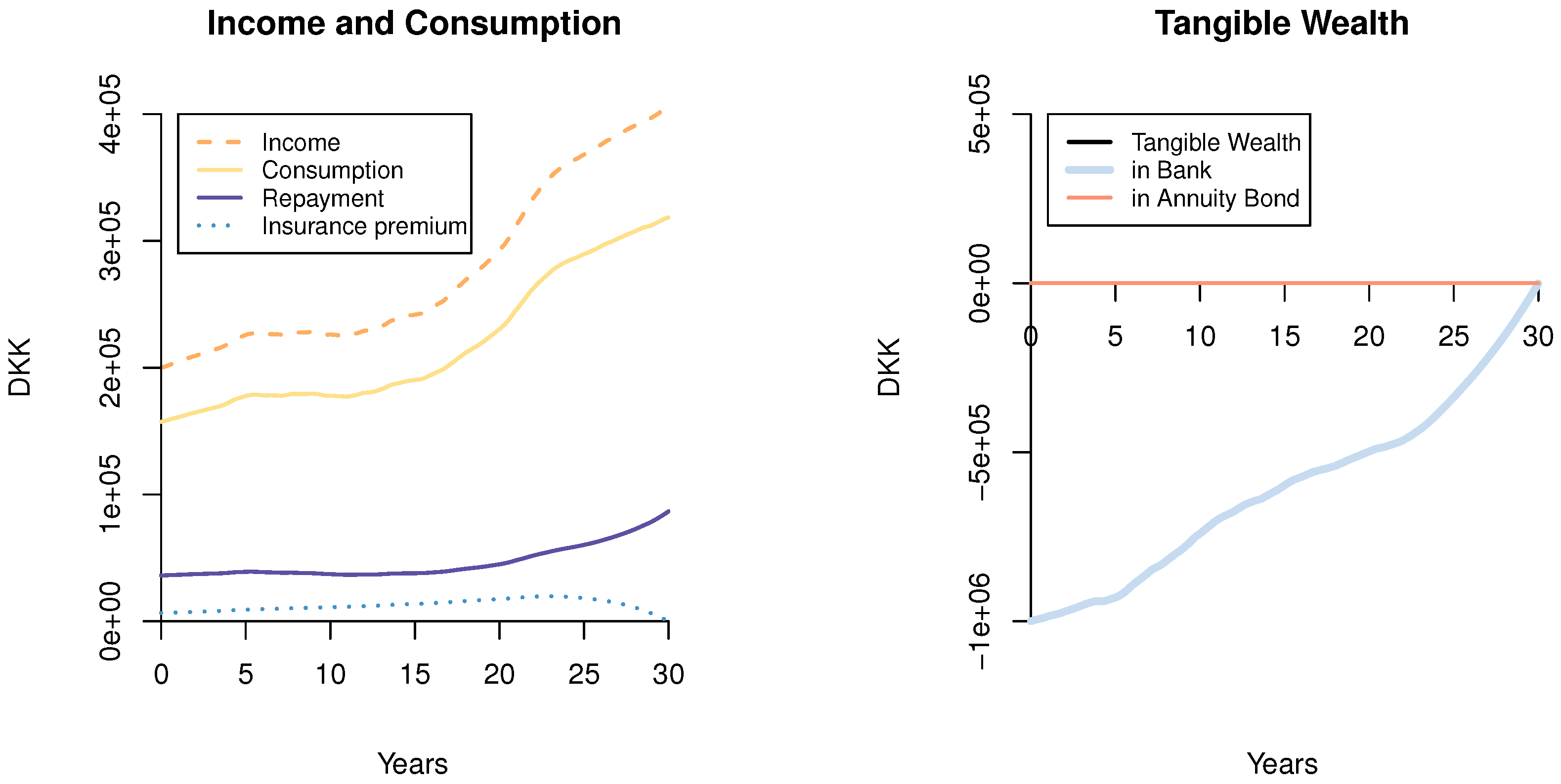
Figure 2 displays a simulation of the consumption and investment of an infinitely risk-averse investor with constant labor income, as described in the previous section, but with the inclusion of mortality. The parameters used for this example are:
It is seen how the optimal payments are almost entirely funded by the FRM. The only thing making the payments non-constant and creating funding in the bank account is the adjustment to account for the insurance premium, as described in the previous section.
6.3. The Moderate FRM Investor
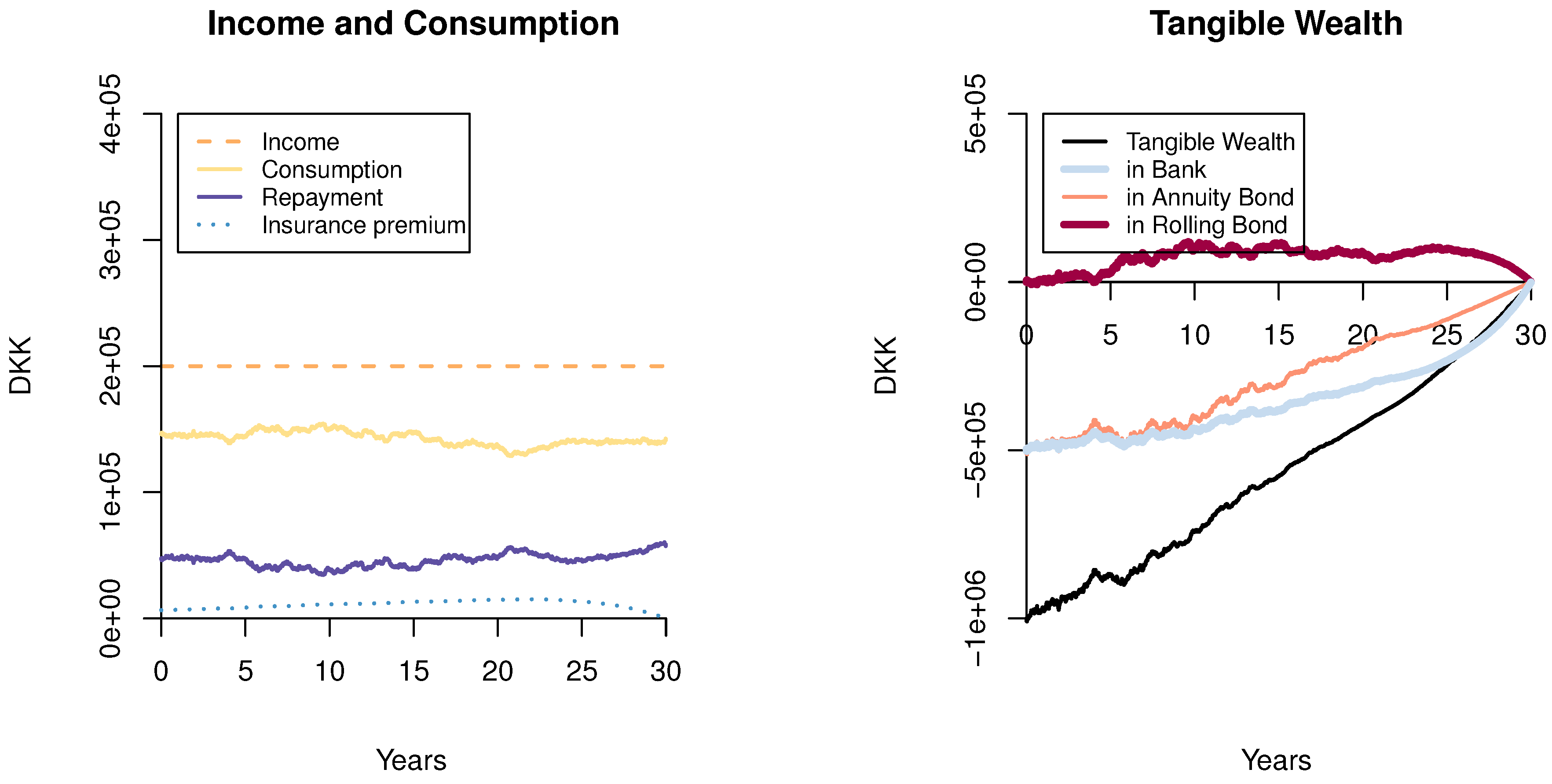
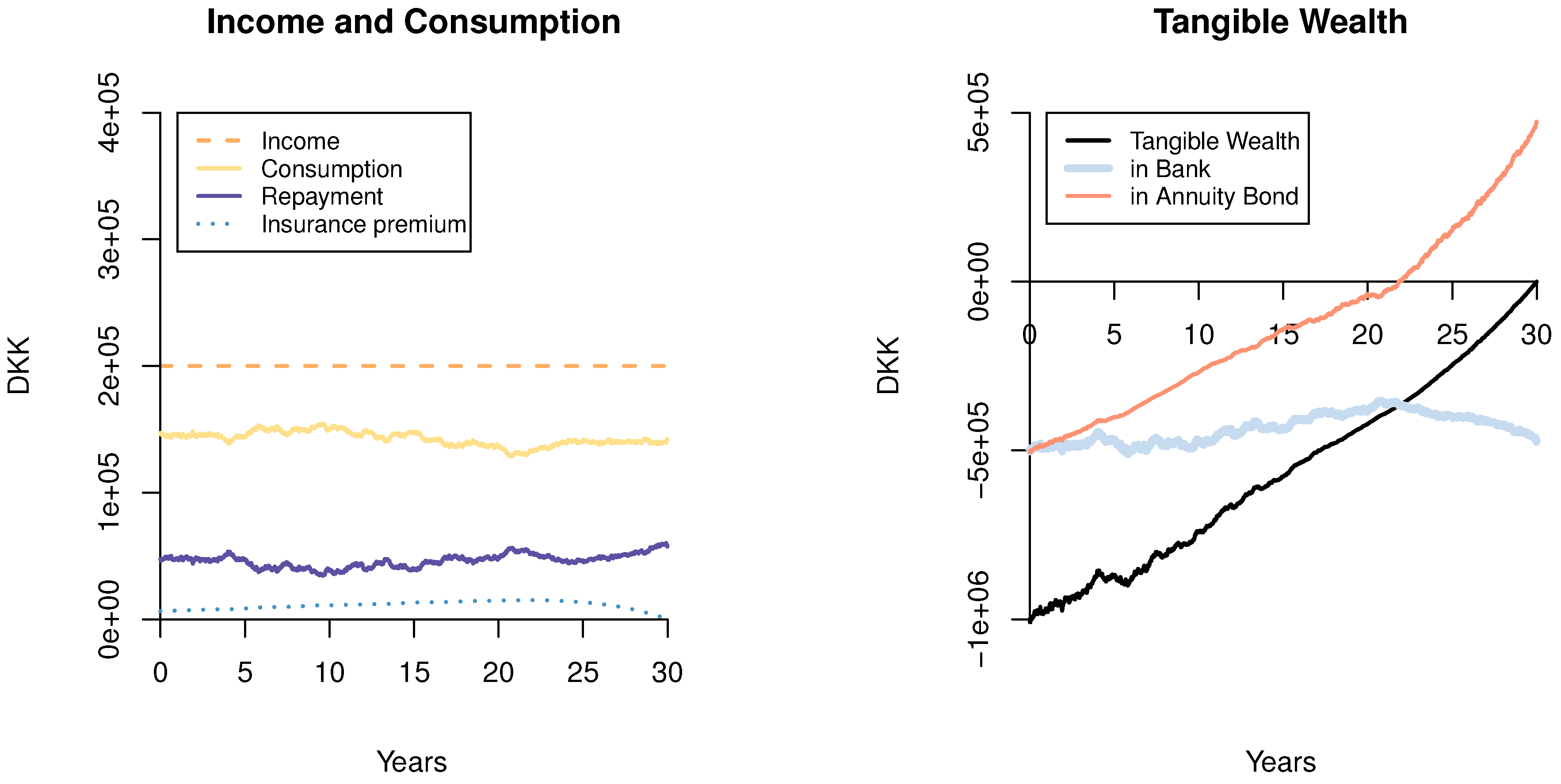
Figure 3 displays a simulation of the consumption and investment of a moderately risk-seeking investor with constant labor income. The parameters used for this example are:
It is seen how a positive speculative demand in the bond emerges towards maturity with a finite risk aversion parameter, as described in the previous sections. It is furthermore observed how the amount of the mortgage funded in the bank account (ARM) is maintained at a fairly constant level throughout the duration of the contract, suggesting an interest-only ARM in combination with positive investment in the annuity bond towards maturity. Since the market value of the annuity bond tends to zero at maturity, this representation is odd when trying to translate it to financial advice. An alternative representation is shown in Figure 4, where the optimal strategy is represented as a mortgage funded in parts by an initial FRM, which is maintained throughout the duration, and in parts by an ARM. Alongside, there is a smaller positive investment in a rolling bond portfolio to adjust for the optimal strategy. This representation is considered to be the most realistic in terms of the borrowing opportunities in the (Danish) market today, where it is very costly to change positions in an FRM due to transaction costs and, hence, not reasonable for the household to change mortgage positions often. Small adjustments like this are better absorbed in personal savings, which are captured as a positive investment in the rolling bond portfolio.
6.4. Effects of the Interest Rate Parameters
Although the study is conducted in a very simple setting, it provides input and intuition on how changing interest rate parameters can affect the optimal mortgage choice. As an example, a large spread between the short-term interest and the implicit long-term interest on an FRM (as determined by Equation (12)) can be invoked by a high long-term mean level and also by a high market price on interest risk, . In this case, with, e.g., and the remaining parameters fixed, it turns out that the moderate FRM investor should optimally choose a higher initial level of FRM coverage, as a result of the total effects on the g- and F-function in Equation (43). This is in contrast to the observed behavior of many mortgagors, as it is documented in Badarinza et al. [10] that the current spread on interest rates on ARM and FRM is the most significant factor in mortgage choice (with ARMs being the favorite when the spread is high). However, if the large yield spread observed in the market is driven by a high market price on interest risk, e.g., , while keeping the other parameters fixed, then the optimal mortgage choice for the moderate FRM investor in our study would be to initially have the entire mortgage funded in the ARM, as a result of the increased positive speculative demand in Equation (43). Therefore, our study indicates that mortgagors should be cautious of choosing increased funding in ARM when the yield spread is high due to a high long-term level of interest, whereas they may enjoy the benefits of an inexpensive ARM, if the high yield spread can be assigned to a high market price on interest risk (in comparison to their own risk appetite). Thus, our study reveals subtle, but important nuances to traditional mortgage advice and provides a simple framework where such effects of market parameters can be studied in more detail and allowing for the development of model-based advice on mortgage choice.
7. Conclusions
This study has provided a closed-form solution to a simple optimal mortgage choice problem. The analytical solution has enabled us to match certain extreme investor characteristics to the two most common products in the market and has enabled a direct analysis of how assumptions regarding preferences, labor income, mortality and market parameters affect the optimal mortgage choice of a household investor. The analysis suggests that households will benefit from a greater flexibility in mortgage repayment profiles. In particular, the profiles should from the outset reflect, e.g., the age of the individual mortgagor and automatically account for the fact that it is optimal for most households to postpone mortgage payments, either due to insurance costs or a known expected increase in income. Furthermore, this study suggests that for a wide range of household investors, the optimal choice in mortgage funding is not either/or in terms of funding in bank account (ARM) vs. annuity bond (FRM), but rather somewhere in between. Therefore, this study recommends that a mix of traditional mortgage products is proposed in the financial advice to households. In particular, this study suggests that investors with a fixed labor income (or fixed available amount for mortgage payments) and a moderate level of risk aversion should choose an FRM in combination with an ARM with flexible repayments alongside a smaller positive bond investment to micro-manage the interest rate risk. We encourage further analytical research on optimal mortgage choice for a greater variety of customer characteristics and market settings.
Acknowledgments
This research has been supported by the Danish Council for Strategic Research (DSF), under Grant No. 10-092299. We thank the two anonymous reviewers for their very helpful comments and suggestions.
Author Contributions
Both authors contributed equally to the paper.
Conflicts of Interest
The authors declare no conflict of interest.
Abbreviations
The following abbreviations are used in this manuscript:
| ARM | Adjustable Rate Mortgage |
| FRM | Fixed Rate Mortgage |
| MLI | Mortgage Life Insurance |
| HJB | Hamilton–Jacobi–Bellman |
Appendix A. Solution to the HJB
Following the usual three steps, presented in, e.g., Korn and Kraft [25]:
- Step 1: Solve the optimization problem of the HJB equation
- Step 2: Insert the result from the optimization and derive the solution to the non-linear PDE (if possible)
- Step 3: Check that all of the assumptions made are able to apply a suitable verification theorem for the HJB applies. With the final step, it is ensured that it is in fact an optimal solution to the problem.
- Step 1:
- Given a solution V to the HJB-equation in (24), this would immediately lead to the optimal consumption:optimal investment:and optimal insurance:due to the restriction that at all times, .
- Step 2:
- Guessing the value function to be in the form of Equation (26) leads to the derivatives:giving optimal consumption:and optimal investment:which coincides perfectly with a simple version of Kraft and Munk [4], when . Determining the exact values of the function g is done by inserting the optimal strategies in the HJB equation in Equation (24). Substantial elimination, using among others the derivative structure of F, results in the following equation:Guessing g to be in the form of Equation (30) again allows deriving the functions and , and the results are given in Equations (32) and (31).
- Step 3:
- As mentioned in Korn and Kraft [25], the usual Lipschitz conditions and linear growth do not hold with the stochastic interest rate; that is why it is necessary to use an extension to the usual verification result of the HJB equation. Such an extension is provided in Kraft [3] and also applies with the addition of perfectly hedgeable labor income and mortality.
References
- R. Korn, and H. Kraft. “A stochastic control approach to portfolio problems with stochastic interest rates.” SIAM J. Control Optim. 40 (2002): 1250–1269. [Google Scholar] [CrossRef]
- C. Munk, and C. Sørensen. “Optimal consumption and investment strategies with stochastic interest rates.” J. Bank. Financ. 28 (2004): 1987–2013. [Google Scholar] [CrossRef]
- H. Kraft. “Optimal portfolios with stochastic short rate: Pitfalls when the short rate is non-Gaussian or the market price of risk is unbounded.” Int. J. Theor. Appl. Financ. 12 (2009): 767–796. [Google Scholar] [CrossRef]
- H. Kraft, and C. Munk. “Optimal housing, consumption, and investment decisions over the life cycle.” Manag. Sci. 57 (2011): 1025–1041. [Google Scholar] [CrossRef]
- J.Y. Campbell, and J.F. Cocco. “Household Risk Management and Optimal Mortgage Choice.” Q. J. Econ. 118 (2003): 1449–1494. [Google Scholar] [CrossRef] [Green Version]
- O. Van Hemert. “Household interest rate risk management.” Real Estate Econ. 38 (2010): 467–505. [Google Scholar] [CrossRef]
- A.M.B. Pedersen, A. Weissensteiner, and R. Poulsen. “Financial planning for young households.” Ann. Oper. Res. 205 (2013): 55–76. [Google Scholar] [CrossRef]
- Z. Bodie, R.C. Merton, and W.F. Samuelson. “Labor supply flexibility and portfolio choice in a life cycle model.” J. Econ. Dyn. Control 16 (1992): 427–449. [Google Scholar] [CrossRef]
- Nationalbanken. Fortsat Overvaegt af Rentefoelsomme Realkreditlaan. Technical Report; Copenhagen, Denmark: Nationalbanken, 2013. [Google Scholar]
- C. Badarinza, J.Y. Campbell, and T. Ramadorai. What Calls to Arms? International Evidence on Interest Rates and the Choice of Adjustable-Rate Mortgages. Technical Report; Cambridge, MA, USA: National Bureau of Economic Research, 2014. [Google Scholar]
- M. Svenstrup, and S. Willemann. “Reforming housing finance: Perspectives from Denmark.” J. Real Estate Res. 28 (2006): 105–130. [Google Scholar] [CrossRef]
- K. Haldrup. “On security of collateral in Danish mortgage finance: A formula of property rights, incentives and market mechanisms.” Eur. J. Law Econ., 2014, 1–29. [Google Scholar] [CrossRef]
- M.E. Yaari. “Uncertain lifetime, life insurance, and the theory of the consumer.” Rev. Econ. Stud. 22 (1965): 137–150. [Google Scholar] [CrossRef]
- S.F. Richard. “Optimal consumption, portfolio and life insurance rules for an uncertain lived individual in a continuous time model.” J. Financ. Econ. 2 (1975): 187–203. [Google Scholar] [CrossRef]
- S.J. Grossman, and G. Laroque. “Asset Pricing and Optimal Portfolio Choice in the Presence of Illiquid Durable Consumption Goods.” Econometrica 58 (1990): 25–51. [Google Scholar] [CrossRef]
- A. Damgaard, B. Fuglsbjerg, and C. Munk. “Optimal consumption and investment strategies with a perishable and an indivisible durable consumption good.” J. Econ. Dyn. Control 28 (2003): 209–253. [Google Scholar] [CrossRef]
- M. Flavin, and S. Nakagawa. “A Model of Housing in the Presence of Adjustment Costs: A Structural Interpretation of Habit Persistence.” Am. Econ. Rev. 98 (2008): 474–495. [Google Scholar] [CrossRef]
- S. Corradin, J.L. Fillat, and C. Vergara-Alert. “Optimal Portfolio Choice with Predictability in House Prices and Transaction Costs.” Rev. Financ. Stud. 27 (2014): 823–880. [Google Scholar] [CrossRef]
- J.B. Baesel, and N. Biger. “The Allocation of Risk: Some Implications of Fixed Versus Index-Linked Mortgages.” J. Financ. Quant. Anal. 15 (1980): 457–468. [Google Scholar] [CrossRef]
- M. Statman. “Fixed Rate or Index-Linked Mortgages from the Borrower’s Point of View: A Note.” J. Financ. Quant. Anal. 17 (1982): 451–457. [Google Scholar] [CrossRef]
- J. Alm, and J.R. Follain. “Alternative mortgage instruments, the tilt problem, and consumer welfare.” J. Financ. Quant. Anal. 19 (1984): 113–126. [Google Scholar] [CrossRef]
- J.K. Brueckner. “Borrower mobility, self-selection, and the relative prices of fixed- and adjustable-rate mortgages.” J. Financ. Int. 2 (1992): 401–421. [Google Scholar] [CrossRef]
- B. Villeneuve. “Mortgage life insurance: A rationale for a time limit in switching rights.” Math. Financ. Econ. 8 (2014): 473–487. [Google Scholar] [CrossRef]
- B. Coulibaly, and G. Li. “Choice of mortgage contracts: Evidence from the survey of consumer finances.” Real Estate Econ. 37 (2009): 659–673. [Google Scholar] [CrossRef]
- R. Korn, and H. Kraft. “On the stability of continuous-time portfolio problems with stochastic opportunity set.” Math. Financ. 14 (2004): 403–414. [Google Scholar] [CrossRef]
Figure 1.
Log-investor with interest- and time-preference-matching labor income and with mortality risk.
Figure 1.
Log-investor with interest- and time-preference-matching labor income and with mortality risk.

Figure 2.
Infinitely risk-averse investor with constant labor income and with mortality risk.
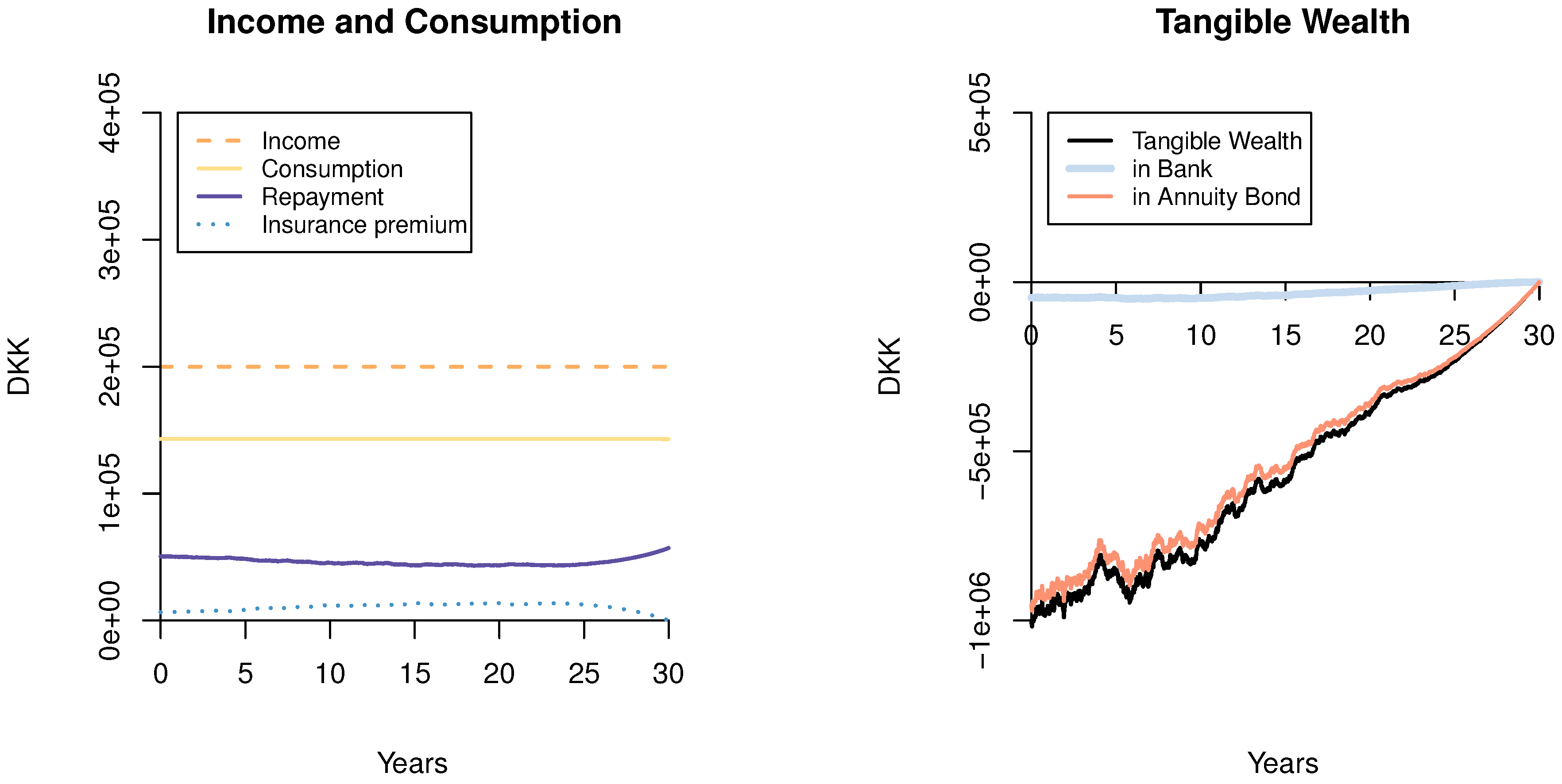
Figure 3.
Moderate investor with constant income in the regular market with mortality risk.

Figure 4.
Investor and strategy identical to Figure 3, but with bond funding expressed as a constant FRM position in combination with a positive investment in the rolling bond.
Figure 4.
Investor and strategy identical to Figure 3, but with bond funding expressed as a constant FRM position in combination with a positive investment in the rolling bond.

Table 1.
Fixed parameters used in all of the numerical examples. The market parameters are consistent with Kraft and Munk [4].
| Parameter | Variable | Value |
|---|---|---|
| Market parameters | ||
| Initial short rate | 0.02 | |
| Mean reversion rate | κ | 0.2 |
| Long-term mean level | 0.02 | |
| Interest volatility | 0.015 | |
| Volatility on rolling bond | 0.0736 | |
| Income parameters | ||
| Volatility | 0 | |
| Constant exponential rate | 0 | |
| Mortality parameters | ||
| Age-independent effect | ||
| Age effect (scale) | ||
| Age effect (exponential) | ||
| Investor parameters | ||
| Investment horizon | T | 30 |
| Age of investor | Age | 50 |
| Initial mortgage size (wealth) | million DKK |
© 2017 by the authors. Licensee MDPI, Basel, Switzerland. This article is an open access article distributed under the terms and conditions of the Creative Commons Attribution (CC BY) license ( http://creativecommons.org/licenses/by/4.0/).
Share and Cite
MDPI and ACS Style
Nordfang, M.-B.; Steffensen, M. Portfolio Optimization and Mortgage Choice. J. Risk Financial Manag. 2017, 10, 1. https://doi.org/10.3390/jrfm10010001
AMA Style
Nordfang M-B, Steffensen M. Portfolio Optimization and Mortgage Choice. Journal of Risk and Financial Management. 2017; 10(1):1. https://doi.org/10.3390/jrfm10010001
Chicago/Turabian StyleNordfang, Maj-Britt, and Mogens Steffensen. 2017. "Portfolio Optimization and Mortgage Choice" Journal of Risk and Financial Management 10, no. 1: 1. https://doi.org/10.3390/jrfm10010001