1. Introduction
Bitcoin, the first decentralized cryptocurrency, has gained a large following from the media, academics and the finance industry since its inception in 2009. Built upon blockchain technology, it has established itself as the leader of cryptocurrencies and shows no signs of slowing down. Instead of being based on traditional trust, the currency is based on cryptographic proof which provides many advantages over traditional payment methods (such as Visa and Mastercard) including high liquidity, lower transaction costs, and anonymity, to name just a few.
Indeed, the global interest in Bitcoin has spiked once again in recent months, for example, the UK government is considering paying out research grants in Bitcoin; an increasing number of IT companies are stockpiling Bitcoin to defend against ransomware; growing numbers in China are buying into Bitcoin and seeing it as an investment opportunity. Perhaps most significantly, the Chair of the Board of Governors of the U.S. Federal Reserve has been encouraging central bankers to study new innovations in the financial industry. In particular, the Chair expressed a need to learn more about financial innovations including Bitcoin, Blockchain, and distributed ledger technologies. With this recent surge in interest, we believe that now is the time to start studying Bitcoin (and other major cryptocurrencies) as key pieces of financial technology.
Since 2009, numerous cryptocurrencies have been developed, with, as of February 2017, 720 in existence. Bitcoin is the largest and most popular representing over 81% of the total market of cryptocurrencies (
CoinMarketCap 2017). However, as the statistics show, many have not garnered the same level of interest. The combined market capitalization of all cryptocurrencies is approximately USD
$19 billion (as of February 2017), with the top 15 currencies representing over 97% of the market, and seven of these accounting for 90% of the total market capitalization. In our analysis, we focus on these seven cryptocurrencies which fall into the category of having existed for more than two years and are within the top 15 currencies by market capitalization. These are Bitcoin, Ripple, Litecoin, Monero, Dash, MaidSafeCoin, and Dogecoin.
There exists much research on Bitcoin—the most popular cryptocurrency. We briefly discuss the analysis and results of some of the most popular studies.
Hencic and Gourieroux (2014) model and predict the exchange rate of Bitcoin versus the U.S. Dollar, using a noncausal autoregressive process with Cauchy errors. Their results show that the daily Bitcoin/USD exchange rate shows local trends which could indicate periods of speculative behaviour from online trading.
Sapuric and Kokkinaki (2014) investigate the volatility of Bitcoin, using data from July 2010 to April 2014, by comparing it to the volatility of the exchange rates of major global currencies. Their analysis indicates that the exchange rate of Bitcoin has high annualised volatility, however, it can be considered more stable when transaction volume is taken into consideration.
Briere et al. (2015) use weekly data from 2010 to 2013 to analyse diversified investment portfolios and find that Bitcoin is extremely volatile and shows large average returns. Perhaps surprisingly, the results indicate that Bitcoin offers little correlation with other assets, although it can help to diversify investment portfolios. In
Kristoufek (2015), the influencing factors of the price of Bitcoin are investigated and applied to the Chinese Bitcoin market. Short and long term links are found, and Bitcoin is shown to exhibit the properties of both standard financial assets but also speculative assets, which fuel further discussion on whether Bitcoin should be classed as a currency, asset or an investment vehicle.
Chu et al. (2015) give the first statistical analysis of the exchange rate of Bitcoin. They fit fifteen of the most common distributions used in finance to the log returns of the exchange rate of Bitcoin versus the U.S. Dollar. Using data from 2011 to 2014 they show that the generalized hyperbolic distribution gives the best fit.
There are thousands of papers published on exchange rates. Hence, it is impossible provide a review of all papers. Here, we mention seven of the most recent papers:
Corlu and Corlu (2015) compare the performance of the generalized lambda distribution against other flexible distributions such as the skewed
t distribution, unbounded Johnson family of distributions, and the normal inverse Gaussian distribution, in capturing the skewness and peakedness of the returns of exchange rates. They conclude that for the Value-at-Risk and Expected Shortfall, the generalised lambda distribution gives a similar performance, and in general it can be used as an alternative for fitting the heavy tail behaviour in financial data;
Nadarajah et al. (2015) revisit the study of exchange rate returns in
Corlu and Corlu (2015), and show that the Student’s
t distribution can give a similar performance to those of the distributions tested in
Corlu and Corlu (2015);
Bruneau and Moran (2017) investigate the effect of exchange rate fluctuations on labour market adjustments in Canadian manufacturing industries;
Dai et al. (2017) examine the role of exchange rates on economic growth in east Asian countries;
Parlapiano et al. (2017) examine exchange rate risk exposure on the value of European firms;
Schroeder (2017) investigates the macroeconomic performance in developing countries with respect to exchange rates;
Seyyedi (2017) provides an analysis of the interactive linkages between gold prices, oil prices, and the exchange rate in India.
One of the aspects we are looking at is the volatility of cryptocurrencies. There are numerous definitions and methods for computing volatility in the literature. For example, in
Sapuric and Kokkinaki (2014) volatility is defined as the annualised volatility (or the standard deviation) representing the daily volatility of an exchange rate. This is calculated by multiplying the standard deviation of the exchange rate by the square root of the number of trading days per year.
Briere et al. (2015) use annualised returns in their analysis and also compute the annualised volatility. Other types of volatility in the literature can be broadly categorised as future, historical, forecast, and implied volatility (
Natenberg 2007). In the remainder of this paper, the term volatility is defined as the spread of the daily exchange rates and log returns of the exchange rates of the cryptocurrencies over the time period considered.
The paper is organised as follows. In
Section 2, we give an overview of the data used in our analysis including descriptions and sources.
Section 3 examines the statistical properties of the cryptocurrencies by fitting a wide range of parametric distributions to the data.
Section 4 provides a discussion of our results. Finally,
Section 5 concludes and summarizes our findings. Throughout the paper, 0.000 should not be interpreted as an absolute zero. It only means that the first three decimal places are equal to zero.
2. Data
The data used in this paper are the historical global price indices of cryptocurrencies, and were obtained from the BNC2 database from Quandl. The global price indices were used as they represent a weighted average of the price of the respective cryptocurrencies using prices from multiple exchanges. For our analysis, we choose to use daily data from 23 June 2014 until the end of February 2017. A start date of June 2014 was deliberately chosen so that we can analyze seven of the top fifteen cryptocurrencies, ranked by their market capitalization, as of February 2017—see
CoinMarketCap (2017) for the current rankings of cryptocurrencies by market capitalization. The seven cryptocurrencies chosen to be part of our analysis are: Bitcoin, Dash, LiteCoin, MaidSafeCoin, Monero, DogeCoin, and Ripple. It should be noted that we omitted Ethereum, arguably the second largest cryptocurrency at present, and Ethereum Classic, as those two only started trading in 2015 and 2016, respectively. Other notable cryptocurrencies such as Agur and NEM were also omitted due to the lack of data. We believe that our choice of cryptocurrencies covers the most prominent currencies, and indeed they represent 90% of the market capitalization as of February 2017 (
CoinMarketCap 2017). In the following, we provide a brief introduction of the seven cryptocurrencies chosen.
Bitcoin is undoubtedly the most popular and prominent cryptocurrency. It was the first realisation of the idea of a new type of money, mentioned over two decades ago, that “uses cryptography to control its creation and transactions, rather than a central authority” (
Bitcoin Project 2017). This decentralization means that the Bitcoin network is controlled and owned by all of its users, and as all users must adhere to the same set of rules, there is a great incentive to maintain the decentralized nature of the network. Bitcoin uses blockchain technology, which keeps a record of every single transaction, and the processing and authentication of transactions are carried out by the network of users (
Bitcoin Project 2017). Although the decentralized nature offers many advantages, such as being free from government control and regulation, critics often argue that apart from its users, there is nobody overlooking the whole system and that the value of Bitcoin is unfounded. In return for contributing their computing power to the network to carry out some of the tasks mentioned above, also known as “mining”, users are rewarded with Bitcoins. These properties set Bitcoin apart from traditional currencies, which are controlled and backed by a central bank or governing body.
Dash (formerly known as Darkcoin and XCoin) is a “privacy-centric digital currency with instant transactions” (
The Dash Network 2017). Although it is based upon Bitcoin’s foundations and shares similar properties, Dash’s network is two-tiered, improving upon that of Bitcoin’s. In contrast with Bitcoin, Dash is overseen by a decentralized network of servers—known as “Masternodes” (
The Dash Network 2017) which alleviates the need for a third party governing body, and allows for functions such as financial privacy and instant transactions. On the other hand, users or “miners” in the network provide the computing power for basic functions such as sending and receiving currency, and the prevention of double spending. The advantage of utilizing Masternodes is that transactions can be confirmed almost in real time (compared with the Bitcoin network) because Masternodes are separate from miners, and the two have non-overlapping functions (
The Dash Network 2017). Dash utilizes the X11 chained proof-of-work hashing algorithm which helps to distribute the processing evenly across the network while maintaining a similar coin distribution to Bitcoin. Using eleven different hashes increases security and reduces the uncertainty in Dash. Dash operates “Decentralized Governance by Blockchain” (
The Dash Network 2017) which allows owners of Masternodes to make decisions, and provides a method for the platform to fund its own development.
LiteCoin (LTC) was created in 2011 by Charles Lee with support from the Bitcoin community. Based on the same peer-to-peer protocol used by Bitcoin, it is often cited as Bitcoin’s leading rival as it features improvements over the current implementation of Bitcoin. It has two main features which distinguish it from Bitcoin, its use of scrypt as a proof-of-work algorithm and a significantly faster confirmation time for transactions. The former enables standard computational hardware to verify transactions and reduces the incentive to use specially designed hardware, while the latter reduces transaction confirmation times to minutes rather than hours and is particularly attractive in time-critical situations (
LiteCoin Project 2017).
MaidSafeCoin is a digital currency which powers the peer-to-peer Secure Access For Everyone (SAFE) network, which combines the computing power of all its users, and can be thought of as a “crowd-sourced internet” (
MaidSafe 2017a). Each MadeSafe coin has a unique identity and there exists a hard upper limit of 4.3 billion coins as opposed to Bitcoin’s 21 million. As the currency is used to pay for services on the SAFE network, the currency will be recycled meaning that in theory the amount of MaidSafe coins will never be exhausted. The process of generating new currency is similar to other cryptocurrencies and in the case of the SAFE network it is known as “farming” (
MaidSafe 2017b). Users contribute their computing power and storage space to the network and are rewarded with coins when the network accesses data from their store (
MaidSafe 2017b).
Monero (XMR) is a “secure, private, untraceable currency” (
Monero 2017) centred around decentralization and scalability that was launched in April 2014. The currency itself is completely donation-based, community driven and based entirely on proof-of-work. Whilst transactions in the network are private by default, users can set their level of privacy allowing as much or as little access to their transactions as they wish. Although it employs a proof-of-work algorithm, Monero is more similar to LiteCoin in that mining of the currency can be done by any modern computer and is not restricted to specially designed hardware. It arguably holds some advantages over other Bitcoin-based cryptocurrencies such as having a dynamic block size (overcoming the problem of scalability), and being a disinflationary currency meaning that there will always exist an incentive to produce the Monero currency (
Monero 2017).
Dogecoin (
Dogecoin 2017) originated from a popular internet meme in December 2013. Created by an Australian brand and marketing specialist, and a programmer in Portland, Oregon, it initially started off as a joke currency but quickly gained traction. It is a variation on Litecoin, running on the cryptographic scrypt enabling similar advantages over Bitcoin such as faster transaction processing times. Part of the attraction of Dogecoin is its light-hearted culture and lower barriers to entry to investing in or acquiring cryptocurrencies. One of the most popular uses for Dogecoin is the tipping of others on the internet who create or share interesting content, and can be thought of as the next level up from a “like” on social media or an “upvote” on internet forums. This in part has arisen from the fact that it has now become too expensive to tip using Bitcoin.
Ripple was originally developed in 2012 and is the first global real-time gross settlement network (RTGS) which “enables banks to send real-time international payments across networks” (
Ripple 2017). The Ripple network is a blockchain network which incorporates a payment system, and a currency system known as XRP which is not based on proof-of-work like Monero and Dash. A unique property of Ripple is that XRP is not compulsory for transactions on the network, although it is encouraged as a bridge currency for more competitive cross border payments (
Ripple 2017). The Ripple protocol is currently used by companies such as UBS, Santander, and Standard Chartered, and increasingly being used by the financial services industry as technology in settlements. Compared with Bitcoin, it has advantages such as greater control over the system as it is not subject to the price volatility of the underlying currencies, and it has a more secure distributed authentication process.
Summary statistics of the exchange rates and log returns of the exchange rates of the seven cryptocurrencies are given in
Table 1 and
Table 2, respectively. In
Table 1, the summary statistics for the raw exchange rates of the cryptocurrencies, we see a simple reflection of the “worth” or value of each currency. It can clearly be seen that the exchange rate of Dogecoin is the least significant, and at the time of writing (February 2017), the exchange rate is approximately
$0.0002 USD to one Dogecoin. This supports the evidence that Dogecoin is primarily used as a currency for online tipping, rather than as a currency for standard payments. It has the lowest minimum, first quartile, median, mean, third quartile, and maximum values. In contrast, being the most popular cryptocurrency, Bitcoin has the largest minimum, first quartile, median, mean, third quartile, and maximum values, which show its greater significance and higher “value” to those with a vested interest in cryptocurrencies. The exchange rates of all seven currencies are positively skewed, with Litecoin, Monero, and Ripple being the most skewed. In terms of kurtosis, MaidSafeCoin shows less peakedness than that of the normal distribution; Bitcoin, Dash, and Dogecoin show levels similar to the normal distribution; Litecoin, Monero, and Ripple have significantly greater peakedness than the normal distribution. The exchange rates of Dogecoin, MaidSafeCoin, and Ripple have the smallest variances and standard deviations, indicating that their low volatility can perhaps be explained by the low values of the exchange rates coupled with the fact that their range and interquartile ranges are very limited. On the other hand, Bitcoin, Dash, and Litecoin’s exchange rates show the greatest variance and standard deviation.
Table 2 gives the summary statistics for the log returns of the exchange rates of the seven cryptocurrencies. Here, the log returns show some slightly different results. Dash, MaidSafeCoin, and Monero have the lowest minimum values, while Dash and Litecoin have the largest maximums. The means and medians of the log returns of all seven currencies are similar and almost equal to zero. Only the log returns of Bitcoin and Litecoin are positively skewed, all others are negatively skewed with Dogecoin being the most significant. Log returns of all seven currencies have a peakedness significantly greater than that of the normal distribution, with the most peaked being those of Dash, Dogecoin, and Litecoin. Noteworthy, as much has been discussed about the volatility of Bitcoin returns, the log returns of Bitcoin have the lowest variance and standard deviation of the seven cryptocurrencies. Those with the highest variation are Dash, and perhaps unexpectedly, MaidSafeCoin and Monero.
Also shown in
Table 1 and
Table 2 are the summary statistics of the exchange rates of the Euro and the summary statistics of its log returns. For the exchange rates, the summary statistics for the Euro appear much smaller than those of Bitcoin but comparable to those of other cryptocurrencies. For the log returns of the exchange rates, the summary statistics for the Euro generally appear smaller compared to all the cryptocurrencies. An exception is the coefficient of variation. The magnitude of this statistic for the Euro appears largest compared to all the cryptocurrencies.
Fitting of a statistical distribution usually assumes that the data are independent and identically distributed (i.e., randomness), have no serial correlation, and have no heteroskedasticity. We tested for randomness using the difference sign and rank tests. We tested for no serial correlation using
Durbin and Watson (
1950,
1951,
1971)’s method. We tested for no heteroskedasticity using
Breusch and Pagan (1979)’s test. These tests showed that the log returns of the exchange rates of the seven cryptocurrencies can be assumed to be approximately independent and identically distributed, have no serial correlation, and have no heteroskedasticity.
3. Distributions Fitted
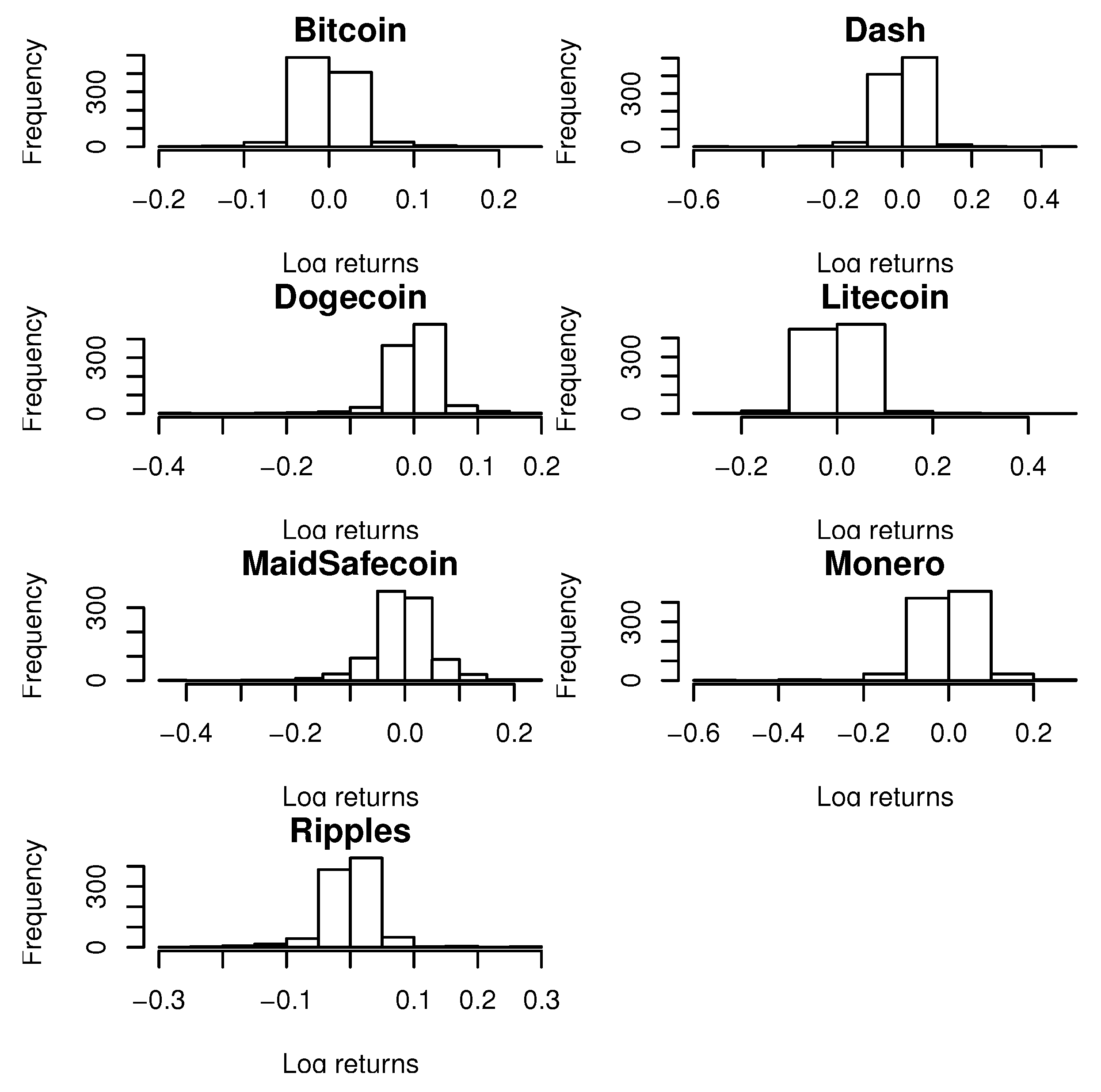
Having briefly examined the summary statistics for both the exchange rates and the log returns of exchange rates of the seven cryptocurrencies, we provide a visual representation of the distribution of the log returns.
Figure 1 shows the histograms of the daily log returns of the exchange rate (versus the U.S. Dollar) for all seven cryptocurrencies. From the plots, we find that the log returns in the cases of all seven cryptocurrencies show significant deviation from the normal distribution. Next, we proceed to fit the parametric distributions to the data.
Let X denote a continuous random variable representing the log returns of the exchange rate of the cryptocurrency of interest. Let denote the probability density function (pdf) of X. Let denote the cumulative distribution function (cdf) of X. We suppose X follows one of eight possible distributions, the most popular parametric distributions used in finance. They are specified as follows:
the Student’s
t distribution (
Gosset 1908) with
for
,
,
and
, where
and
denotes the beta function defined by
the Laplace distribution (
Laplace 1774) with
for
,
and
;
the skew
t distribution (
Azzalini and Capitanio 2003) with
for
,
,
,
and
, where
denotes the Gauss hypergeometric function defined by
where
denotes the ascending factorial;
the generalized
t distribution (
McDonald and Newey 1988) with
for
,
,
,
and
;
the skewed Student’s
t distribution (
Zhu and Galbraith 2010) with
for
,
,
and
;
the asymmetric Student’s
t distribution (
Zhu and Galbraith 2010) with
for
,
,
,
and
, where
the normal inverse Gaussian distribution (
Barndorff-Nielsen 1977) with
for
,
,
,
and
, where
and
denotes the modified Bessel function of the second kind of order
defined by
where
denotes the modified Bessel function of the first kind of order
defined by
where
denotes the gamma function defined by
the generalized hyperbolic distribution (
Barndorff-Nielsen 1977) with
for
,
,
,
,
and
, where
.
Many of these distributions are nested: the skew t distribution for is the Student’s t distribution; the generalized t distribution for is the Student’s t distribution; the skewed Student’s t distribution for is the Student’s t distribution; the asymmetric Student’s t distribution for is the skewed Student’s t distribution; the generalized hyperbolic distribution for is the normal inverse Gaussian distribution; and so on.
All but one of the distributions (the Laplace distribution) are heavy tailed. Heavy tails are common in financial data. The Student’s
t distribution is perhaps the simplest of the heavy tailed distributions. It does not allow for asymmetry. The skew
t distribution due to
Azzalini and Capitanio (2003) is an asymmetric generalization of the Student’s
t distribution. The generalized
t distribution due to
McDonald and Newey (1988) has two parameters controlling its heavy tails, adding more flexibility. The skewed Student’s
t distribution due to
Zhu and Galbraith (2010) is a generalization of the Student’s
t distribution with the scale allowed to be different on the two sides of
. This distribution is useful if positive log returns have a different scale compared to negative log returns. The asymmetric Student’s
t distribution due to
Zhu and Galbraith (2010) is a generalization of the Student’s
t distribution with the scale as well as the tail parameter allowed to be different on the two sides of
. This distribution is useful if positive log returns also have a different heavy tail behavior compared to negative log returns. The generalized hyperbolic distribution due to
Barndorff-Nielsen (1977) accommodates semi heavy tails. It is popular in finance because it contains several heavy tailed distributions as particular cases.
The maximum likelihood method was used to fit each distribution. If
is a random sample of observed values on
X and if
are parameters specifying the distribution of
X then the maximum likelihood estimates of
are those maximizing the likelihood
or the log likelihood
where
denotes the pdf of
X. We shall let
denote the maximum likelihood estimate of
. The maximization was performed using the routine optim in the R software package (
R Development Core Team 2017). The standard errors of
were computed by approximating the covariance matrix of
by the inverse of observed information matrix, i.e.,
Many of the fitted distributions are not nested. Discrimination among them was performed using various criteria:
the Akaike information criterion (
Akaike 1974) defined by
the Bayesian information criterion (
Schwarz 1978) defined by
the consistent Akaike information criterion (CAIC) (
Bozdogan 1987) defined by
The five discrimination criteria above, used to discriminate between and determine the best fitting distribution, all utilise the maximum likelihood estimate. In all cases, the smaller the values of the criteria the better the fit. The Akaike information criterion comprises two parts: the bias (log likelihood) and variance (parameters) (
Hu 2007), and the larger the log likelihood the better the goodness of fit. However, the criterion includes a penalty term which is dependent on the number of parameters in the model. This penalty term increases with the number of estimated parameters and discourages overfitting. The Bayesian information criterion is very similar to that of the Akaike information criterion, the only difference being that the penalty term is not twice the number of estimated parameters, but instead is the number of parameters multiplied by the natural logarithm of the number of observed data points. The two criteria possess different properties and thus their use is also dependent on different factors. In addition, the Bayesian information criterion is asymptotically efficient, while the Akaike information criterion is not (
Vrieze 2012). The consistent Akaike information criterion and the corrected Akaike information criterion are also very similar to both the Akaike and Bayesian information criteria. The former acts as a direct extension of the Akaike information criterion in that it is asymptotically efficient and still includes a penalty term which penalises overfitting more strictly (
Bozdogan 1987). On the other hand, the latter includes a correction for small sample bias and includes an additional penalty term which is a function of the sample size (
Anderson et al. 2010). Finally, an alternative to the Akaike and Bayesian information criteria is the Hannan-Quinn information criterion. The expression for the Hannan-Quinn criterion is the same as that for the Akiake information criterion, however, the parameter term is multiplied by the double logarithm of the sample size. In general, the Hannan-Quinn criterion penalises models with a greater number of parameters more compared to both the Akaike and Bayesian information criteria. However, it tends to show signs of overfitting when the sample size is small (
McNelis 2005). For a more detailed discussion on these criteria, see
Burnham and Anderson (2004) and
Fang (2011).
Apart from the five criteria, various other measures could be used to discriminate between non-nested models. These could include:
the Kolmogorov-Smirnov statistic (
Kolmogorov 1933;
Smirnov 1948) defined by
where
denotes the indicator function and
the maximum likelihood estimate of
;
the Anderson-Darling statistic (
Anderson and Darling 1954) defined by
where
are the observed data arranged in increasing order;
Once again the smaller the values of these statistics the better the fit. The use of these statistics in
Section 4 instead of the five criteria led to the same conclusions.
4. Results
In this section, we provide our analysis in terms of the best fitting distributions and the results for the log returns of the different cryptocurrencies. The results provided are in terms of log likelihood values, information criteria, goodness of fit tests, probability plots, quantile plots, plots of two important financial risk measures, back-testing using Kupiec’s test and dynamic volatility.
4.1. Fitted Distributions and Results
The eight distributions in
Section 3 were fitted to the data described in
Section 2. The method of maximum likelihood was used. The parameter estimates and their standard errors for the best fitting distributions in each case are given in
Table 3. The log likelihood values, and the values of AIC, AICc, BIC, HQC and CAIC for the fitted distributions (for each of the seven cryptocurrencies) are shown in
Table 4,
Table 5,
Table 6,
Table 7,
Table 8,
Table 9 and
Table 10. We find that there is no one best fitting distribution jointly for all seven cryptocurrencies. However, we find that for Bitcoin (the most popular cryptocurrency) and its nearest rival LiteCoin, the generalized hyperbolic distribution gives the best fit. For three out of the seven: Dash, Monero, and Ripple, the normal inverse Gaussian distribution gives the best fit. For Dogecoin and MaidSafeCoin, the best fitting distributions are the generalized
t and Laplace distributions, respectively. The adequacy of the best fitting distributions is assessed in terms of Q-Q plots, P-P plots, the one-sample Kolmogorov-Smirnov test, the one-sample Anderson-Darling test and the one-sample Cramer-von Mises test.
The best fitting distributions show the following: log returns of the exchange rates of MaidSafeCoin have light tails; log returns of the exchange rates of Dogecoin have heavy tails; log returns of the exchange rates of Bitcoin, Dash, Litecoin, Monero and Ripple have semi heavy tails. Among the last five, the asymmetry of tails as measured by is negative for Dash, Monero and Ripple. Of these the largest asymmetry is for Dash, followed by Monero and then Ripple. The asymmetry of tails as measured by is positive for Bitcoin and Litecoin. Of these the larger asymmetry is for Bitcoin.
It is surprising that a light tailed distribution (the Laplace distribution) gives the best fit for log returns of the exchange rates of MaidSafeCoin. However, many authors have found that the Laplace distribution can provide adequate fits to financial data:
Linden (2001) models stock returns by the Laplace distribution;
Linden (2005) models the realized stock return volatility by the Laplace distribution;
Aquino (2006) establishes that the Laplace distribution characterizes the price movements for the Philippine stock market;
Podobnik et al. (2009) show Laplace distribution fits for the stock growth rates for the Nasdaq Composite and the New York Stock Exchange Composite.
All of the cryptocurrencies show substantially larger volatility than the exchange rate of the Euro. Nevertheless, we also observe substantial differences within the group of cryptocurrencies. The distribution of the tails of their returns ranges from light tailed via semi-heavy tailed to heavy tailed. Given that traditional financial instruments usually exhibit heavy tails, this is a slightly surprising, but also a very important, result.
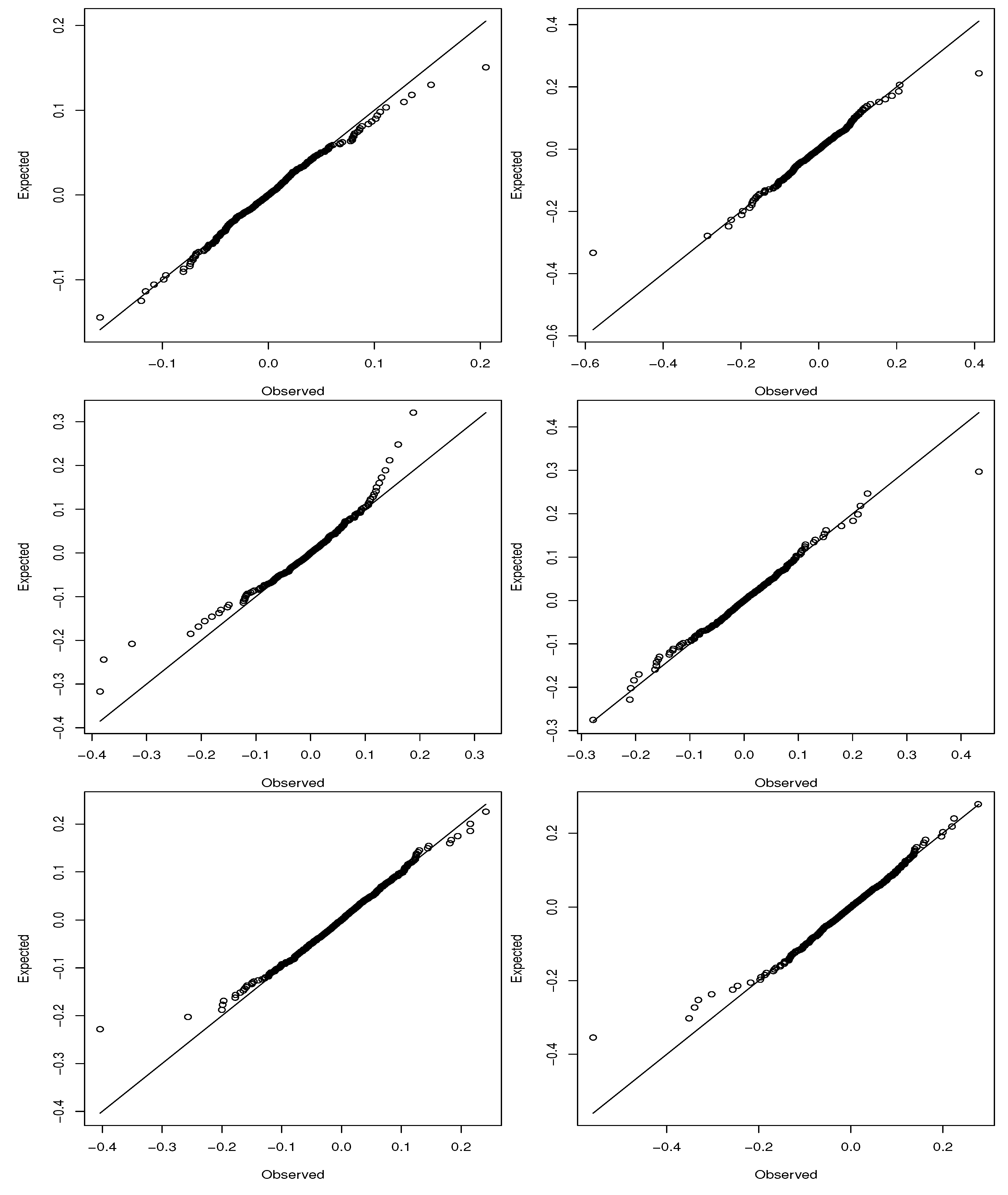
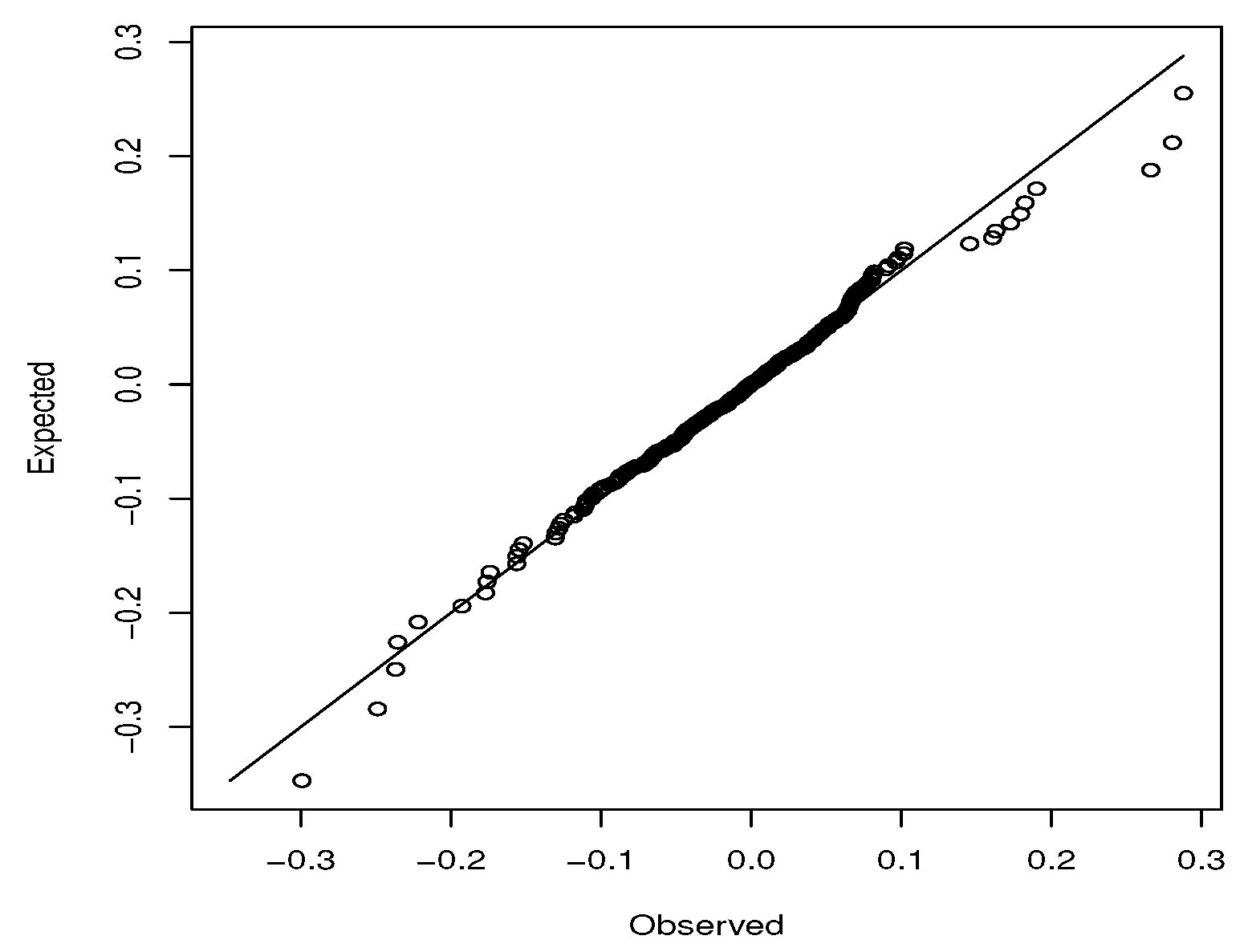
4.2. Q-Q Plots
The Q-Q plots for the best fitting distribution for each of the seven cryptocurrencies are shown in
Figure 2. For Bitcoin, the best fitting distribution captures the middle and lower parts of the data well but not the upper tail. For Dash, the best fitting distribution captures the middle, lower and upper parts of the data well. For Dogecoin, the best fitting distribution captures the middle part of the data well but not the lower or upper tails. For Litecoin, the best fitting distribution captures the middle, lower and upper parts of the data well. For MaidSafeCoin, the best fitting distribution captures the middle and upper parts of the data well but not the lower tail. For Monero, the best fitting distribution captures the middle and upper parts of the data well but not the lower tail. For Ripple, the best fitting distribution captures the middle part of the data well but not the lower or upper tails.
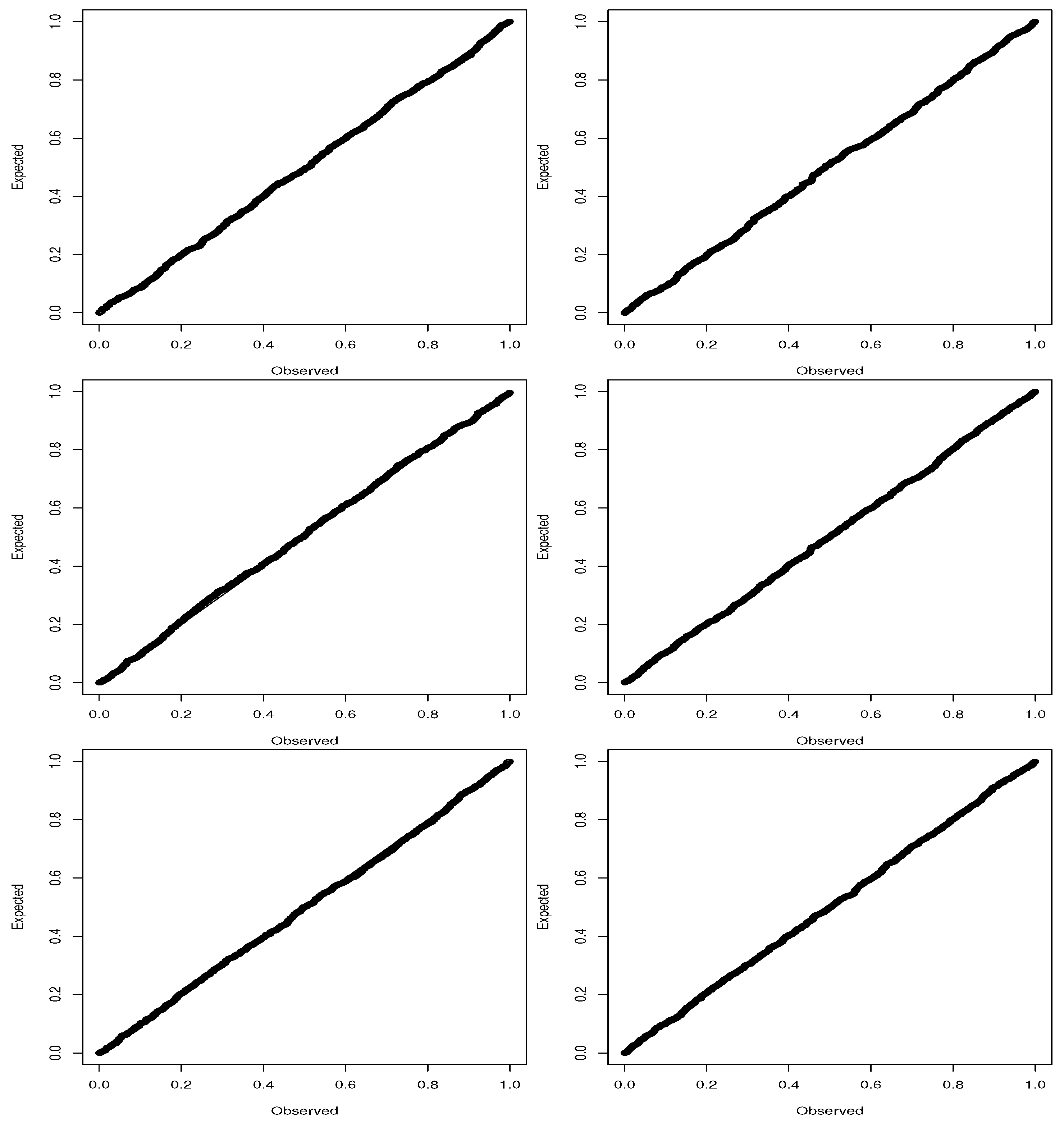
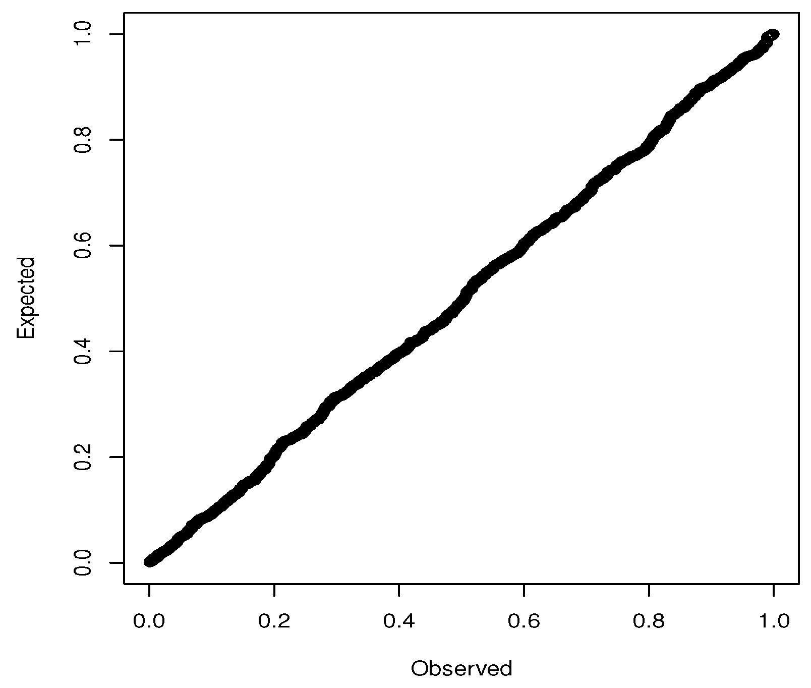
4.3. P-P Plots
The P-P plots for the best fitting distribution for each of the seven cryptocurrencies are shown in
Figure 3. For each cryptocurrency, the best fitting distribution captures the middle, lower and upper parts of the data well.
4.4. Goodness of Fit Tests
The
p-values of the one-sample Kolmogorov-Smirnov test for the best fitting distributions listed in
Table 3 are 0.095, 0.124, 0.164, 0.094, 0.119, 0.162 and 0.056. The corresponding
p-values of the one-sample Anderson-Darling test are 0.103, 0.144, 0.154, 0.120, 0.051, 0.157 and 0.176. The corresponding
p-values of the one-sample Cramer-von Mises test are 0.082, 0.116, 0.196, 0.085, 0.168, 0.088 and 0.122. Hence, all of the best fitting distributions are adequate at the five percent significance level.
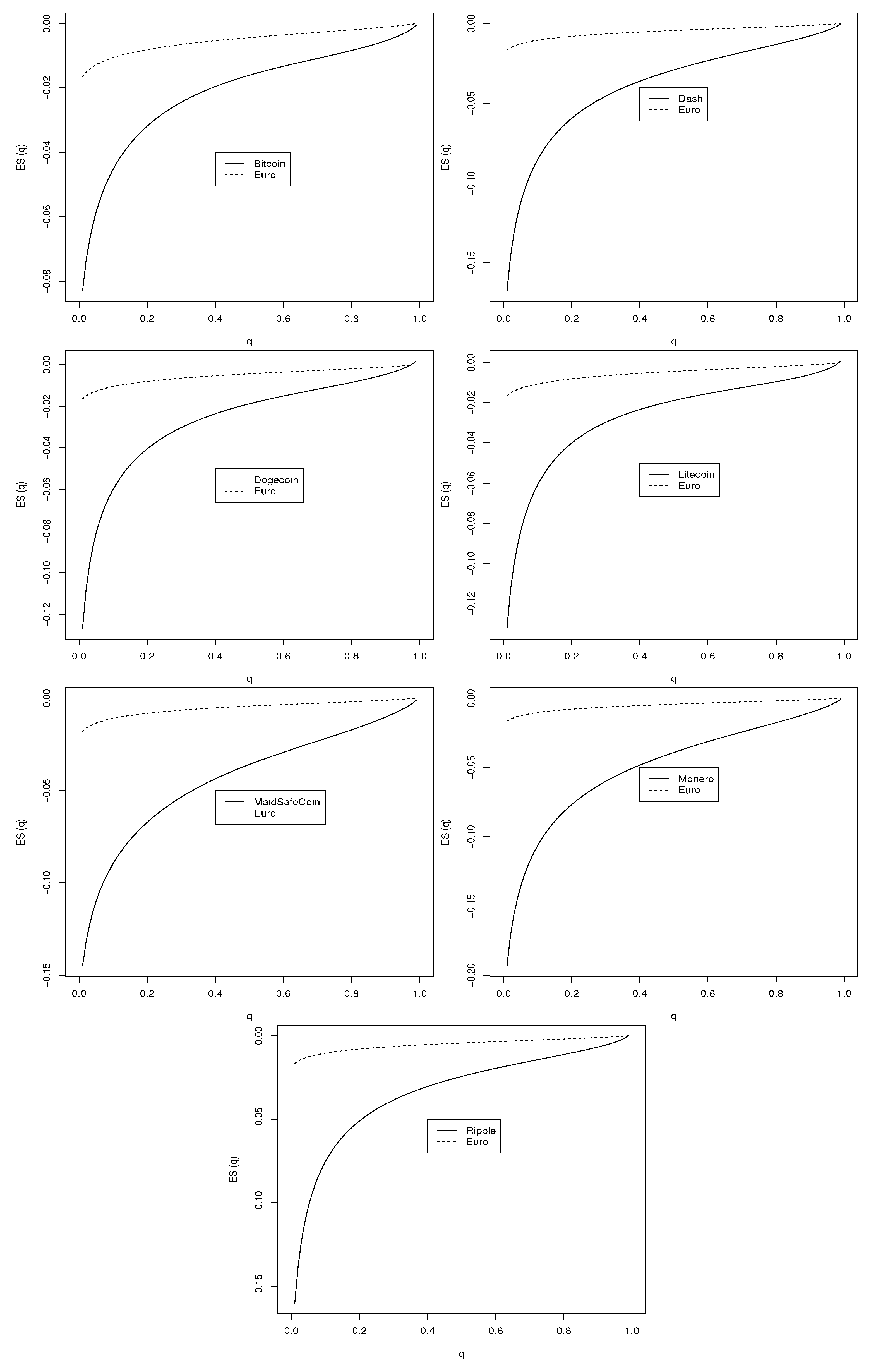
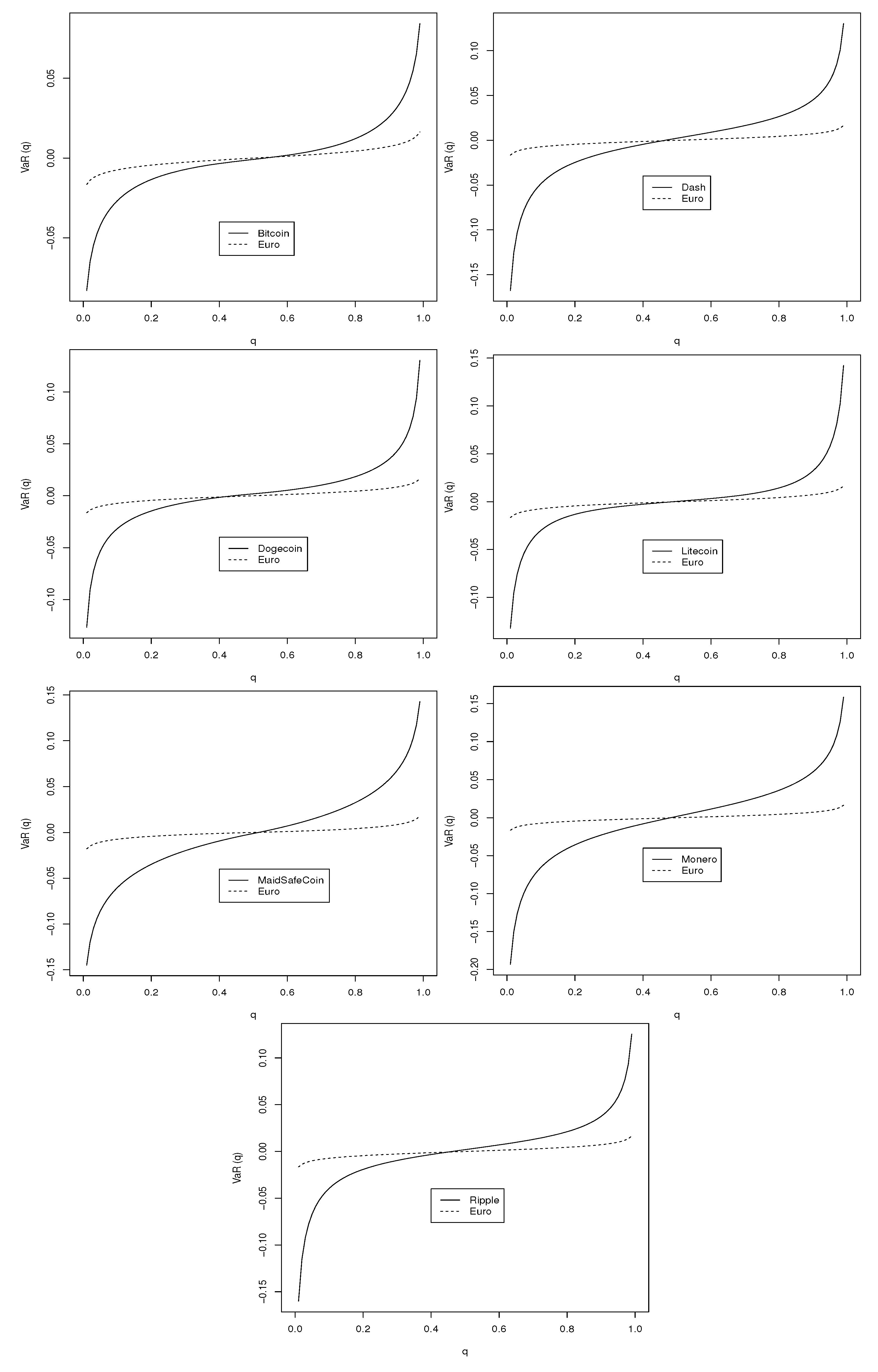
4.5. VaR and ES Plots
Value at risk (VaR) and expected shortfall (ES) are the two most popular financial risk measures (
Kinateder 2015,
2016). If
denotes the cdf of the best fitting distribution then VaR and ES corresponding to probability
q can be defined by
and
respectively, for
. Plots of VaR
and ES
for the best fitting distributions for the seven cryptocurrencies are shown in
Figure 4 and
Figure 5. Also shown in the figures are estimates of VaR
and ES
for daily log returns of the Euro computed using the same best fitting distributions. It is clear that each cryptocurrency is riskier than the Euro. With respect to the upper tail of VaR, Litecoin, MainSafecoin and Monero appear to have the largest risks. With respect to the lower tail of VaR, Monero appears to have the largest risk. Monero also has the largest risk with respect to the lower tail of ES.
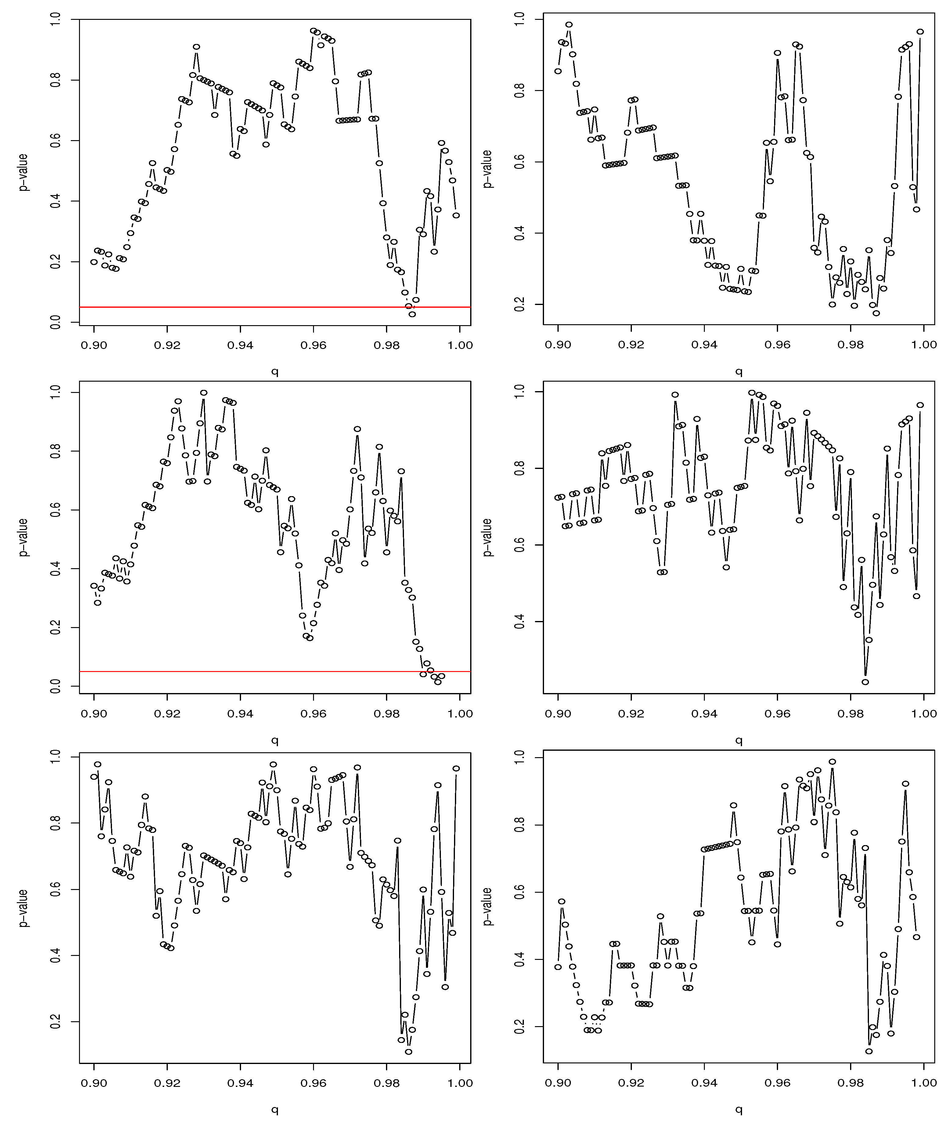
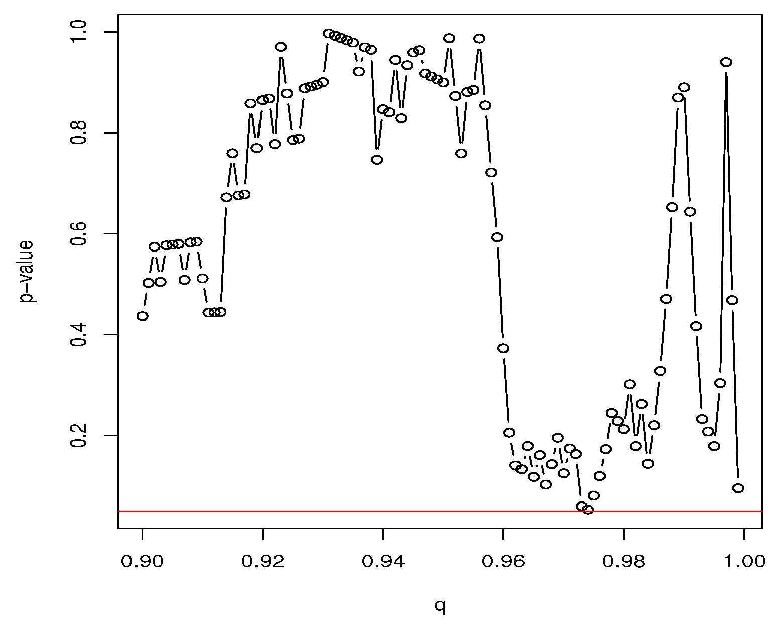
4.6. Kupiec’s test
The
p-values of Kupiec’s test for the best fitting distribution for each of the seven cryptocurrencies are shown in
Figure 6. The
p-values (points above 0.05 in
Figure 6) suggest that the out of sample performance of VaR can be considered accurate at the corresponding values of
q for any of the best fitting distributions. The motivation for using the Kupiec’s test is that we can give predictions of the exchange rate of the different cryptocurrencies, including predictions for the extreme worst case scenario and the extreme best case scenario.
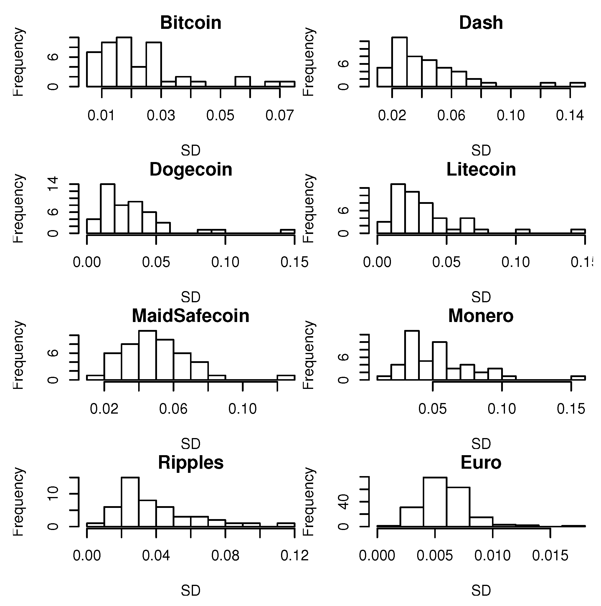
4.7. Dynamic Volatility
So far in this section, we have supposed that volatility is represented by a fixed parameter of a distribution. Often in financial series, volatility varies throughout time. This could be accommodated in various ways. One is to treat volatility itself as a random variable. Another is to let volatility depend on some covariates including time as in GARCH models for example. In the first case, the interest will be on the distribution of volatility.
For the seven cryptocurrencies and the Euro, we computed standard deviations of daily log returns of the exchange rates over windows of width 20 days. Histograms of these standard deviations are shown in
Figure 7. We see that the distribution is skewed for the seven cryptocurrencies and the Euro. The range of volatility appears smallest for the Euro and second smallest for Bitcoin. The range appears largest for Dogecoin, Litecoin and Monero.


