Recovering Historical Inflation Data from Postage Stamps Prices


Econometric Institute, Erasmus School of Economics, Burgemeester Oudlaan 50, 3062PA Rotterdam, The Netherlands
*
Author to whom correspondence should be addressed.
J. Risk Financial Manag. 2017, 10(4), 21; https://doi.org/10.3390/jrfm10040021
Submission received: 17 October 2017
/
Revised: 7 November 2017
/
Accepted: 9 November 2017
/
Published: 14 November 2017
(This article belongs to the Special Issue Applied Econometrics)
Abstract
:For many developing countries, historical inflation figures are rarely available. We propose a simple method that aims to recover such figures of inflation using prices of postage stamps issued in earlier years. We illustrate our method for Suriname, where annual inflation rates are available for 1961 until 2015, and where fluctuations in inflation rates are prominent. We estimate the inflation rates for the sample 1873 to 1960. Our main finding is that high inflation periods usually last no longer than 2 or 3 years. An Exponential Generalized Autoregressive Conditional Heteroscedasticity (EGARCH) model for the recent sample and for the full sample with the recovered inflation rates shows the relevance of adding the recovered data.
JEL Codes:
E31; N10; N161. Introduction and Motivation
The World Bank collects annual inflation rates for all countries in the world. For developed countries, such data can be available for a long span of time, also because statistical bureaus for the countries exist for a long time.1 For many developing countries, matters can be different. For example, Benin’s first available inflation figure concerns 1993, whereas Ethiopia’s first quote concerns 1966. There may be various causes for this lack of data, which can relate to a lack of institutions and the effects of decolonization.
For various reasons, one may want to have some impression of historical figures. One would perhaps want to know if a current high inflation period, which indicates a period with risky economic fluctuations, has occurred before and which measures were taken to reduce inflation. Alternatively, one may want to compare inflation patterns across countries to discern similarities or specific differences. In addition, one may want to compute historical data on real GDP, real wages, and purchasing power parity, which all involve price levels. Preferably, one would also want to have annual data without missing data in between.
Recovering historical price levels can be difficult because of lack of information on the prices of many goods and because good and services may have changed substantially over the years. Various recent studies present discussions of methods to recover historical data and the reliability of those historical statistics, see Allen et al. (2011), Bolt and van Zanden (2014), Cendejas Bueno and Font de Villanueva (2015), Deaton and Heston (2010), Frankema and van Waijenburg (2012), and Jerven (2009).
In the present paper, we present a new and very simple method that aims to reconstruct historical inflation rates. We seek to alleviate the issue of changing products over time by considering a product that has not much changed over time and for which prices are immediately available. This product concerns postage stamps. First, postage stamps have been issued in many countries for a long time. Next, the type of product and its use did not change much over the years. In addition, evidently, the price of the stamp is printed on the stamp; see for example Figure 1, where we present a few stamps for Suriname.
In the present paper, and only for illustrative purposes, we consider the historical prices of this South American country, which borders Guyana and Brazil. The World Bank can provide us with annual inflation rates starting in 1961. The first stamps in Suriname were issued in 1873, and hence we aim to retrieve annual inflation rates since that year. We chose Suriname as the estimation sample because it is reasonably large, ranging from, 1961 to and including 2015, as there were many stamps issued per year, and also as there is substantial variation in the inflation figures over time. It also so happens that, at the time of writing this paper in 2016, inflation is again very high, and people may wonder how long high inflation periods typically last.
The outline of our paper is as follows. Section 2 deals with the inflation rates data and with the stamps data, and provides some characteristics. Section 3 deals with two types of models to see if (changes in) postal stamps prices have explanatory value for inflation. One model is a simple regression model, while the other is a MIDAS regression, which fits annual inflation rates to quarterly stamps prices.2 Both models suggest strong predictive power of the stamps prices. Section 4 deals with the backward extrapolation and identifies a few historical periods with excessive inflation rates and their potential causes. Section 5 concludes.
2. The Data
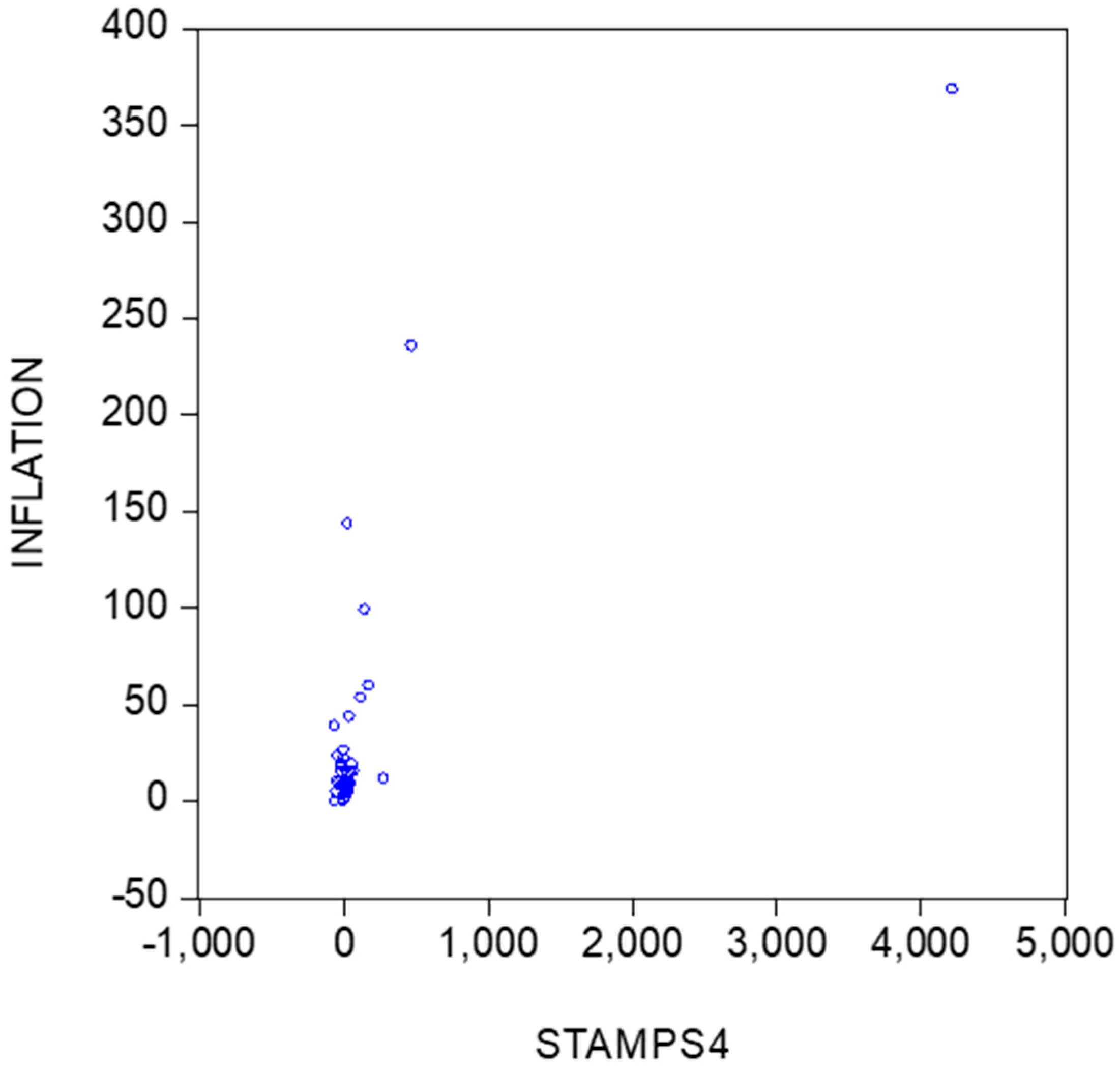
The annual inflation rates for 1961 to 2015 for Suriname are retrieved from the World Bank. Table 1 presents the data, and Figure 2 visualizes the data. Clearly, the data show periods with high inflation, and 1994 stands out with an inflation rate of 368.5 per cent. This number associates with approximately 1.6 per cent per day. Periods with high inflation are 1993 to 1995 and 1999 to 2001, while 1987 was also an exceptional year. The International Monetary Fund provides a review of the potential causes for the high inflation rates in the nineties.3
Table 2 presents the data on the postage stamps, also for the period 1961 to 2015. We consulted two catalogues, and retrieved the median prices of all the stamps in each year. The first catalogue runs until 12 November 1975, a few weeks before Suriname became an independent country on 25 November 1975. Before independence, Suriname was a colony of the Netherlands since the 17th century. The first postage stamp in Suriname was issued in 1873.
The data in Table 2 show that, like inflation, the percentage changes in postal stamp prices can be substantial. The observation in 1994 stands out with a value of 4220.99 per cent. In various years, we also see that price changes were equal to zero.
3. Two Econometric Models
In this section, we consider two econometric models to link inflation with changes in stamp prices. We denote annual inflation as and the annual changes in stamps prices as . For inflation, we have only annual data, but for the stamps prices, we can also construct quarterly data. Each year, a range of stamps was issued, and this allows us to construct quarterly percentage changes, as the catalogues give the exact dates (day, month, and year) of issue. There are now two ways to compute these changes in postal stamps prices. The first refer a current quarter with the previous quarter—that is, the first-order differences. We denote these as , where T again corresponds with years and q with the quarters 1, 2, 3, and 4. The data appear in Figure 5. The second type of percentage changes concern the differences between a current quarter and the same quarter the year before. We denote these as , as these concern fourth-order differences. The data are depicted in Figure 6.
At first, we allow for potential differences across models for the periods before and after the date of independence, and we thus start with the following regression model for the data from 1975 onwards, that is
where is annual inflation and as are the annual changes in stamps prices. The estimation results for the sample 1975 to 2015 appear in the first panel of Table 3. The parameters are estimated using Ordinary Least Squares (OLS), with Newey-West adjusted standard errors. The tests for normality and first-order residual autocorrelation indicate that the model can be improved. A closer look at the residuals reveals that there are (at least) two very large residuals, concerning 1993 and 1999. The second panel of Table 3 displays the estimation results for the case where lagged inflation is deleted (as it was not significant) and where the observations in 1993 and 1999 are not included. The test results now suggest that the model is appropriately specified. The last panel of Table 3 presents the results for the same model, but now for the sample starting in 1961. Even though the tests do diagnose some problems with the errors (which are due to some modest outliers), the parameter estimates for current and lagged changes in stamps prices are remarkably constant across models and samples.
To see if data that are more detailed can lead to better models, we consider two MIDAS models. The first model is
where is the first-order differenced median stamps prices, where T again corresponds with years and q with the quarters 1, 2, 3, and 4. The OLS estimation results, with Newey-West adjusted standard errors, for this model are given in the left panel of Table 4. The diagnostic tests for normality and first-order residual autocorrelation suggest that this model is adequately specified.
The second MIDAS model is
where are the fourth-order differenced median stamps prices, where T again corresponds with years and q with the quarters 1, 2, 3 and 4. The OLS estimation results, with Newey-West adjusted standard errors, are in the second panel of Table 4. This MIDAS model also seems to fit the data well. When we compare the in-sample prediction errors, we see that the difference in accuracy is small. Given that the diagnostic tests indicate appropriate models, we learn that adding higher frequency terms to the regression models leads to more accuracy.
Overall, the estimation results in this section show that inflation and changes in stamps prices are strongly connected, at least here for the case of Suriname. Because the frequency of publication of the postal stamps before 1975 is lower, the MIDAS models however are not useful for the purpose we have in mind, namely recovering historical inflation rates, despite the increased accuracy they offered.
4. Recovery of Historical Inflation Rates
Given that, a suitable model for annual inflation rates appears to be
we will use the parameter estimates in the final panel of Table 3 to make backward predictions for inflation. That is, for the sample 1873 to 1960, we compute
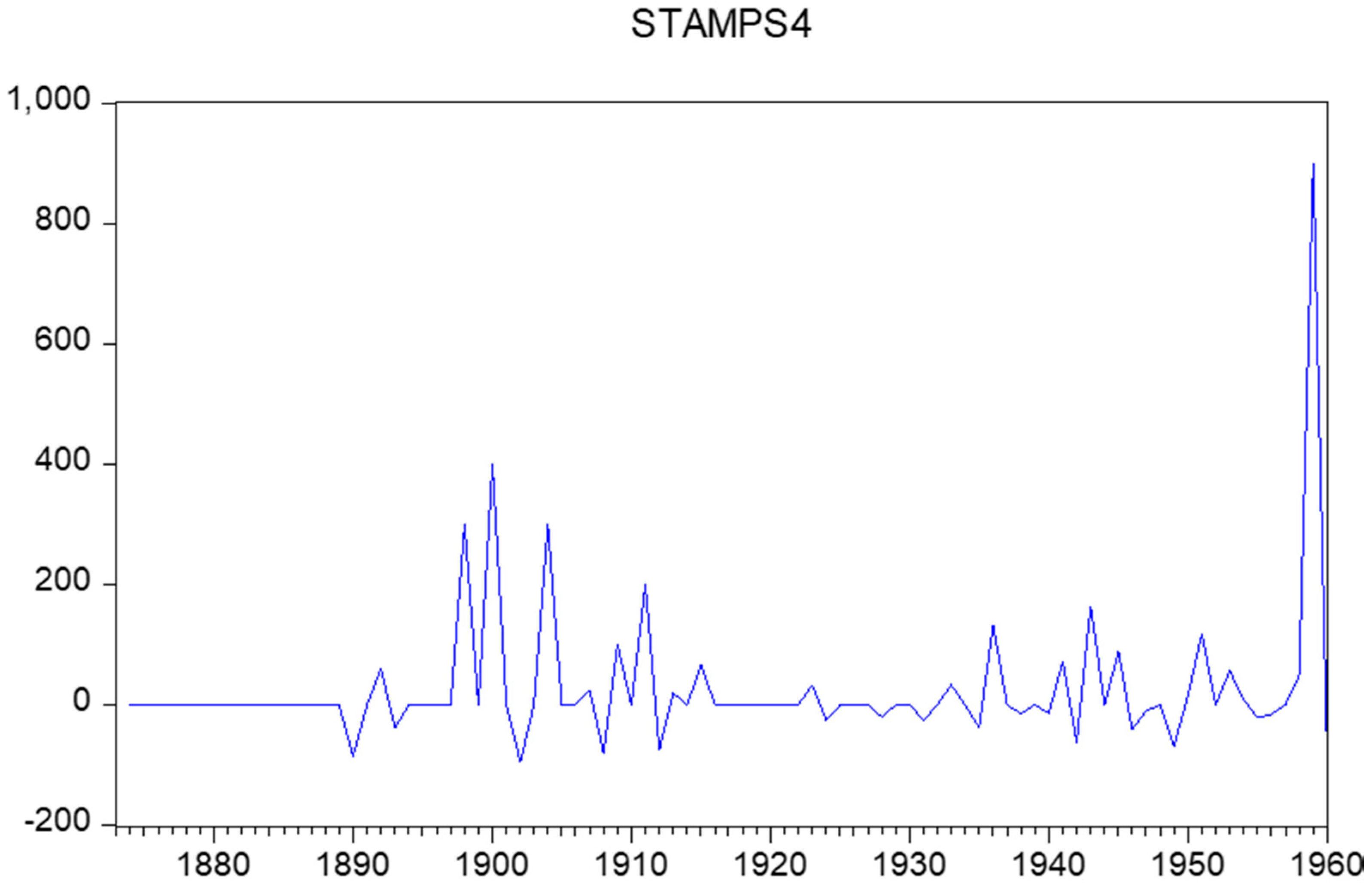
Figure 7 displays the observations on the changes in the postal stamps prices for these years, which were collected from the first mentioned catalogue in Table 2. In addition, Figure 8 displays the estimated historical inflation observations.
We see that high inflation periods each time last for usually one or one years, and at most four years (Figure 9). Specifically, if we define a high inflation period as a period with inflation higher than 10 per cent, the average length of such a period is 1.45 using the fitted sample from 1873–2015.
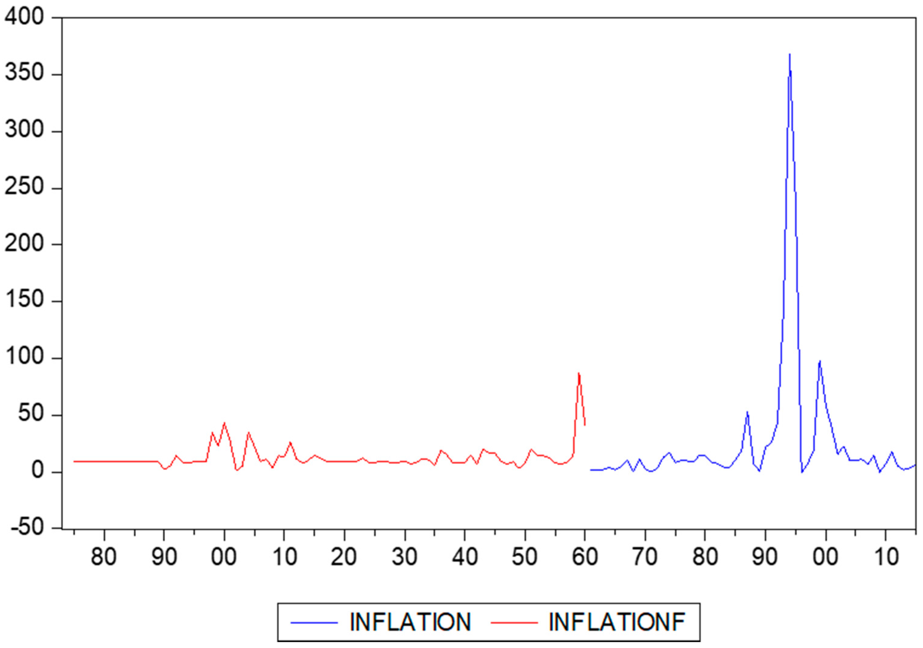
Figure 10 displays the actual data from 1961 onward and the estimated data back to 1873 in one single graph. Clearly, the data in the nineties are exceptional. Postal stamps experienced enormous price changes during the 1990s. This period exactly coincides with the hyperinflation that Suriname experienced during that time.
However, various other periods in our forecasting sample are characterized by high inflation rates. Consider for example the 1900s, 1930s, 1940s, and 1950s (specifically 1957). In Table 5, more details on these periods are discussed. The high inflation rates around 1900 coincides with the gold rush at the same time at the Lawa River in Suriname, which amounted to higher tariffs for transportation (see Van Velzen and Hoogbergen (2013)). The higher inflation rates in the 1930s can be related to a period of economic decline and austerity measures, causing social upheaval (Hoefte 2013). The developments in 1940s can be most likely attributed to the consequences of the Second World War. The very high inflation rates as indicated by the peak at 1957 occur in the same year as the establishment of the central bank of Suriname,4 but certainly coincides with the so-called Eisenhower recession.
Finally, Table 6 presents the estimation results of an EGARCH model, measuring risk.5 The model reads as
where covers the full sample from 1873 to 2015, with
in addition, is a standard normally distributed variable. We need to add 1 to where to make sure that all observations are positive. The estimation results (with Bollerslev-Wooldridge robust standard errors in parentheses) for the sample 1961–2015 and the full sample (1873–2015) with the recovered data shows reasonably similar parameter estimates and much smaller estimated standard errors in the latter case. This seems to support the quality of the recovered inflation figures.
with
Estimated using Eviews package 8.0. To reduce the effect of outliers, the data are transformed as indicated. Bollerslev-Wooldridge robust standard errors are in parentheses.
5. Conclusions
We proposed a simple method to estimate annual historical data on inflation using changes in postal stamps prices. The method seems to work, at least for Suriname. A next step would be to reconstruct historical figures for other countries. If possible, we would want to match our estimates with actually observed inflation rates, should those data be available.
Author Contributions
Philip Hans Franses and Eva Janssens collected the data, performed the analysis and Philip Hans Franses and Eva Janssens wrote the paper.
Conflicts of Interest
The authors declare no conflict of interest.
References
- Allen, Robert C., Jean-Pascal Bassino, Debin Ma, Christine Moll-Murata, and Jan Luiten van Zanden. 2011. Wages, prices, and living standards in China, 1738–1925: In comparison with Europe, Japan, and India. Economic History Review 64: 8–38. [Google Scholar] [CrossRef] [Green Version]
- Andreou, Elena, Eric Ghysels, and Andros Kourtellos. 2010. Regression models with mixed sampling frequencies. Journal of Econometrics 158: 246–61. [Google Scholar] [CrossRef]
- Bolt, Jutta, and Jan Luiten van Zanden. 2014. The Maddison Project: Collaborative research on historical national accounts. Economic History Review 67: 627–51. [Google Scholar] [CrossRef]
- Cendejas Bueno, Jose Luis, and Cecilia Font de Villanueva. 2015. Convergence of inflation with a common cycle: Estimating and modelling Spanish historical inflation from the 16th to the 18th centuries. Empirical Economics 48: 1643–65. [Google Scholar] [CrossRef]
- Chang, Chia-Lin, and Michael McAleer. 2017. The correct regularity condition and interpretation of asymmetry in EGARCH. Economics Letters 161: 52–55. [Google Scholar] [CrossRef]
- Clements, Michael P., and Anna B. Galvao. 2008. Macroeconomic forecasting with mixed-frequency data. Journal of Business and Economic Statistics 26: 546–54. [Google Scholar] [CrossRef]
- Deaton, Angus, and Alan Heston. 2010. Understanding PPPs and PPP-based national accounts. American Economic Journal: Macroeconomics 2: 1–35. [Google Scholar] [CrossRef]
- Frankema, Ewout H. P., and Marlous van Waijenburg. 2012. Structural impediments to African growth? New evidence from real wages in British Africa, 1880–1965. Journal of Economic History 72: 895–926. [Google Scholar] [CrossRef]
- Franses, Philip Hans, and Rianne Legerstee. 2014. Statistical institutes and economic prosperity. Quality and Quantity 48: 507–20. [Google Scholar] [CrossRef]
- Ghysels, Eric, Pedro Santa-Clara, and Rossen Valkanov. 2004. The MIDAS Touch: Mixed Data Sampling Regression Models. CIRANO Working Paper 2004s-20. Montreal, QC, Canada: CIRANO. [Google Scholar]
- Ghysels, Eric, Arthur Sinko, and Rossen Valkanov. 2007. Midas regressions: Further results and new directions. Econometric Reviews 26: 53–90. [Google Scholar] [CrossRef]
- Hoefte, Rosemarijn. 2013. Suriname in the Long Twentieth Century: Domination, Contestation, Globalization. Berlin: Springer. [Google Scholar]
- Jerven, Morten. 2009. The relativity of poverty and income: How reliable are African economic statistics? African Affairs 109: 77–96. [Google Scholar] [CrossRef]
- McAleer, Michael, and Christiaan Hafner. 2014. A one line derivation of EGARCH. Econometrics 2: 92–97. [Google Scholar] [CrossRef] [Green Version]
- Van Velzen, Thoden, and Wim Hoogbergen. 2013. Een Zwarte Vrijstaat in Suriname (Deel 2): De Okaanse Samenleving in de Negentiende en Twintigste Eeuw. Leiden: Brill. [Google Scholar]
| 1 | See Franses and Legerstee (2014) for a table with dates for 106 countries when statistical bureaus were founded. |
| 2 | Important references to MIDAS regression are Andreou et al. (2010), Clements and Galvao (2008), Ghysels et al. (2004), and Ghysels et al. (2007). |
| 3 | |
| 4 | |
| 5 | See Chang and McAleer (2017) and McAleer and Hafner (2014) for two recent studies on this very useful model. |
Figure 1.
A few stamps issued in 1996 in Suriname (with exceptionally high prices).

Figure 2.
Inflation (in yearly percentages) in Suriname.
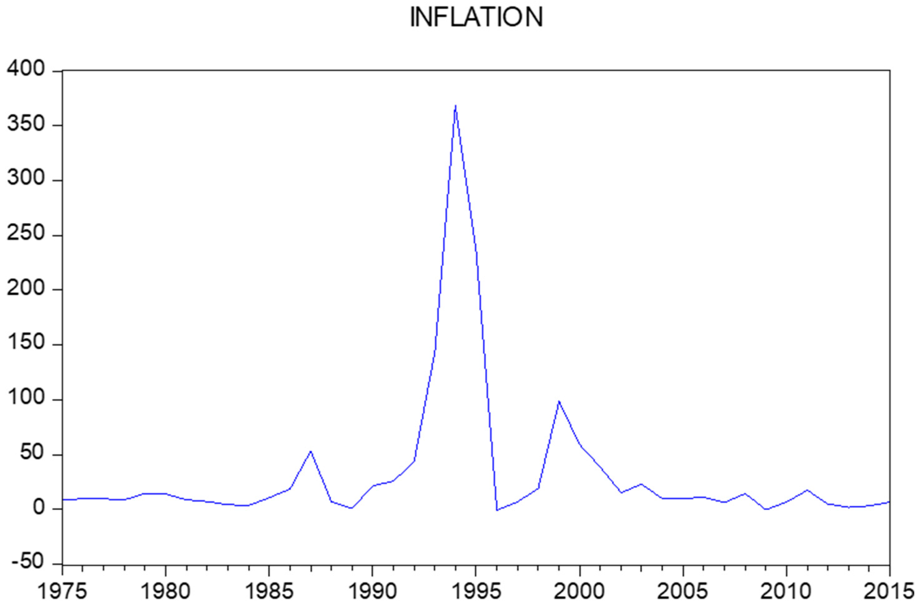
Figure 3.
Scatter of inflation versus percentage changes in stamps prices (all observations).

Figure 4.
Scatter of inflation versus percentage changes in stamps prices (excluding 1994).
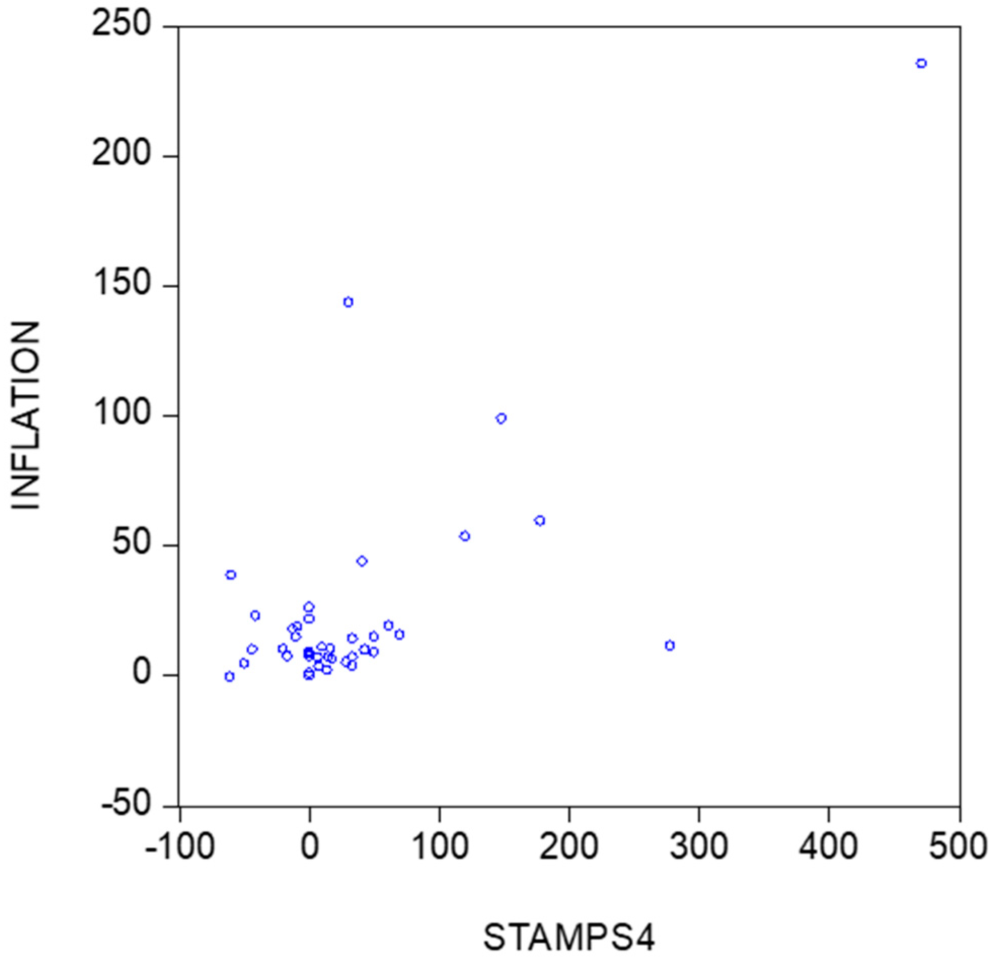
Figure 5.
Quarter-to-quarter changes in stamps prices for MIDAS regression.
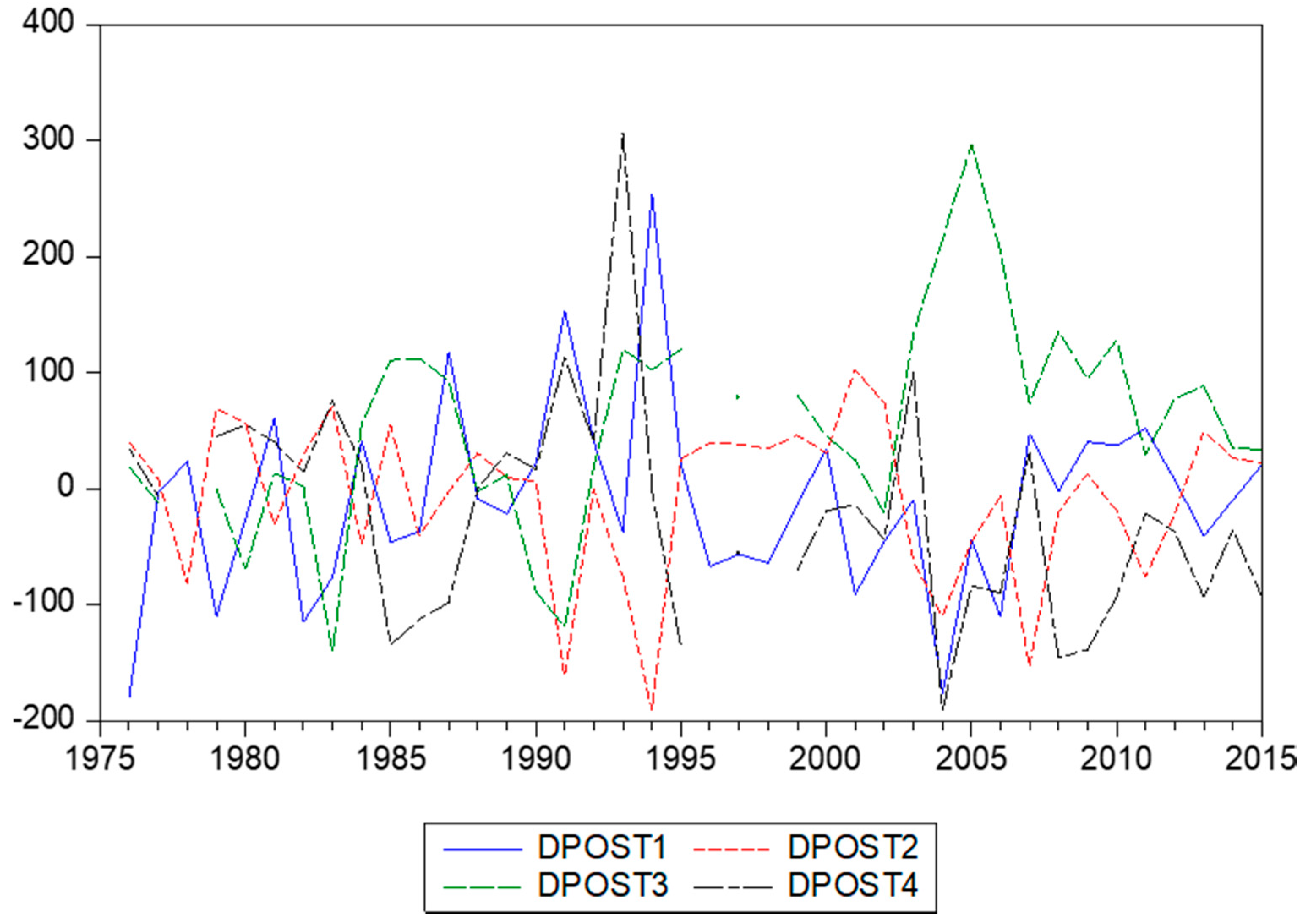
Figure 6.
Annual changes in stamps prices, observed per quarter, for MIDAS regression.
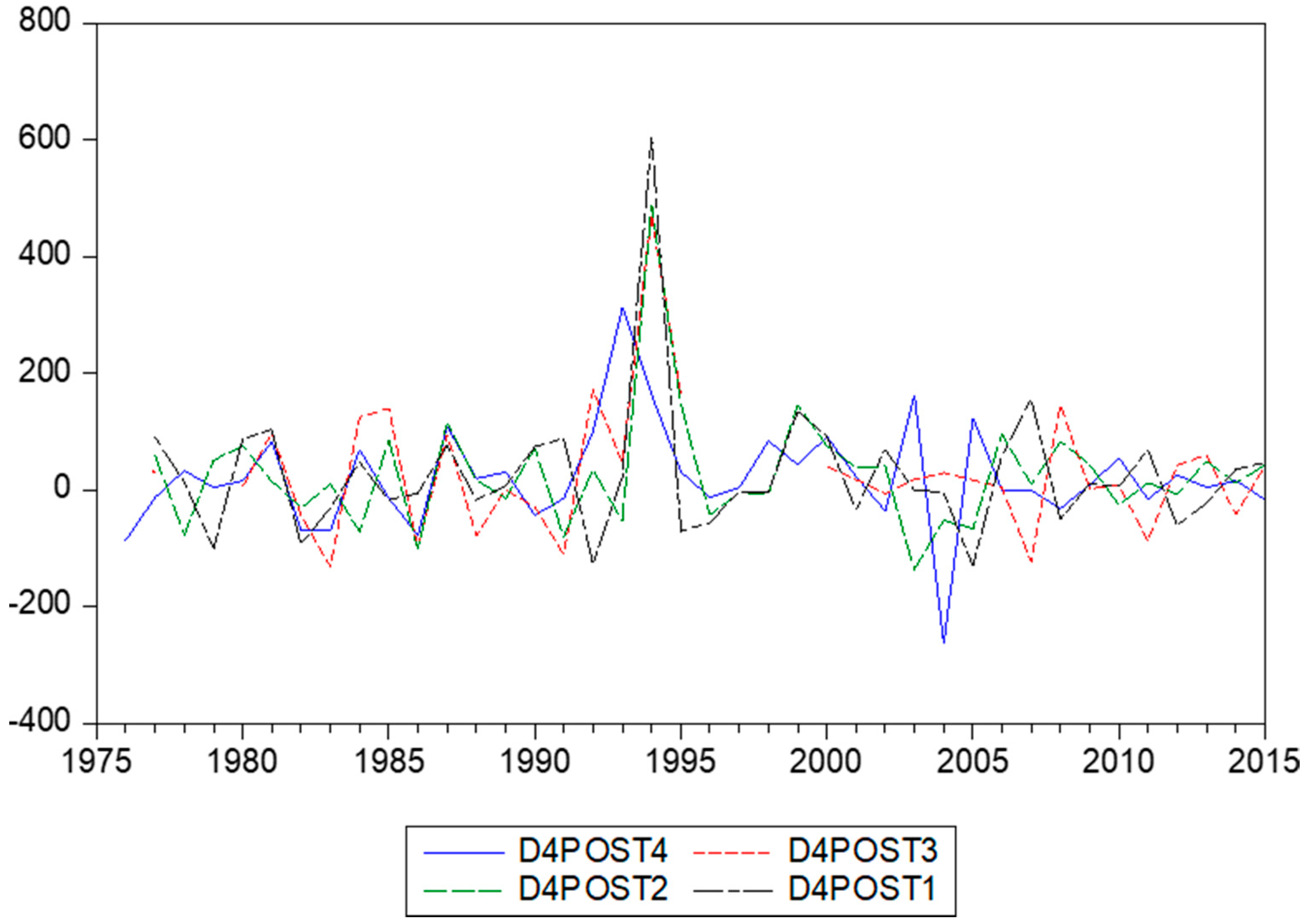
Figure 7.
Percentage changes in postal stamps prices, 1873–1960.

Figure 8.
Predictions of inflation rates for 1873 to 1960.
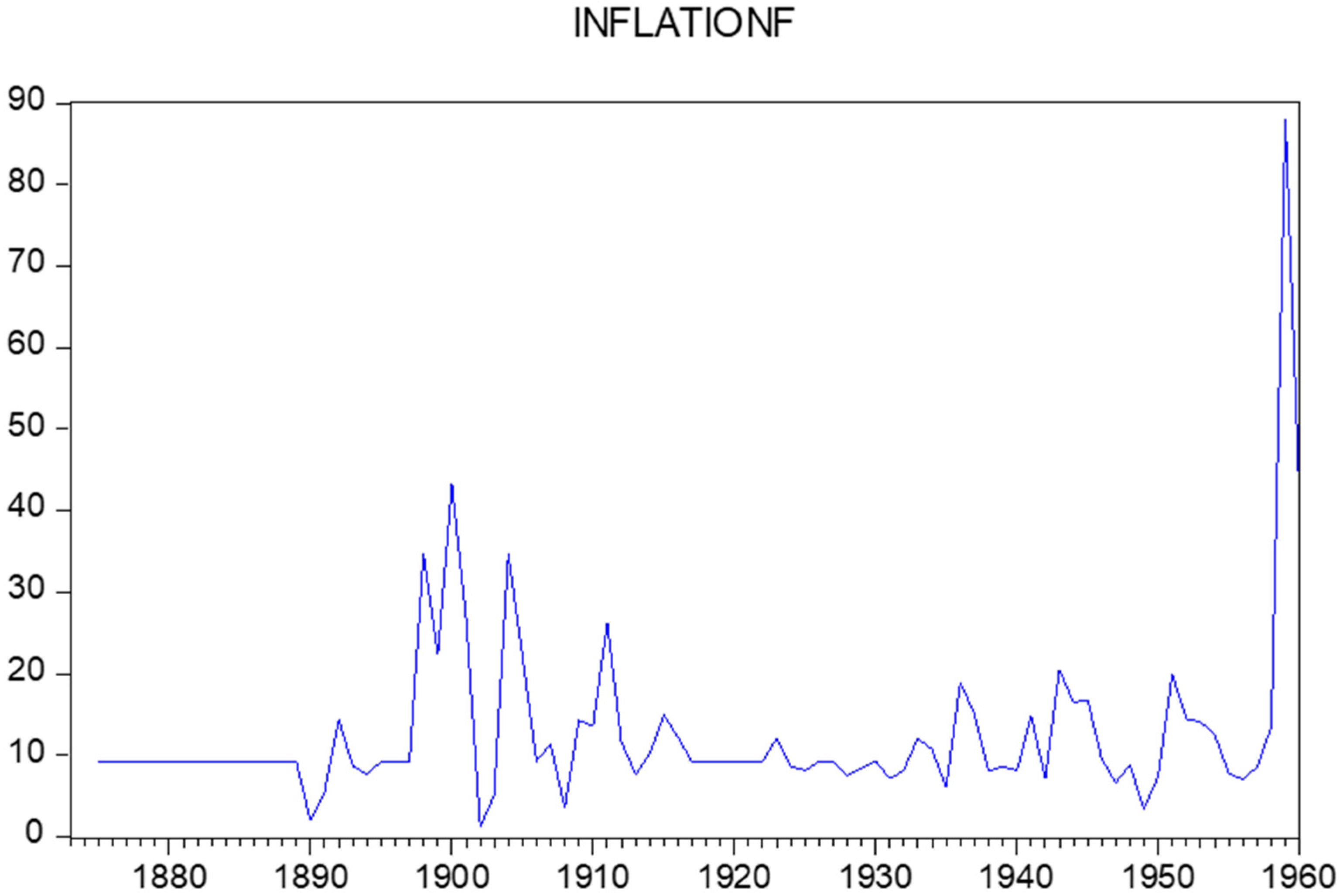
Figure 9.
Length of periods with high inflation rates (inflation above 10 per cent) and their frequency of occurrence, based on fitted sample of 1873–2015.
Figure 9.
Length of periods with high inflation rates (inflation above 10 per cent) and their frequency of occurrence, based on fitted sample of 1873–2015.
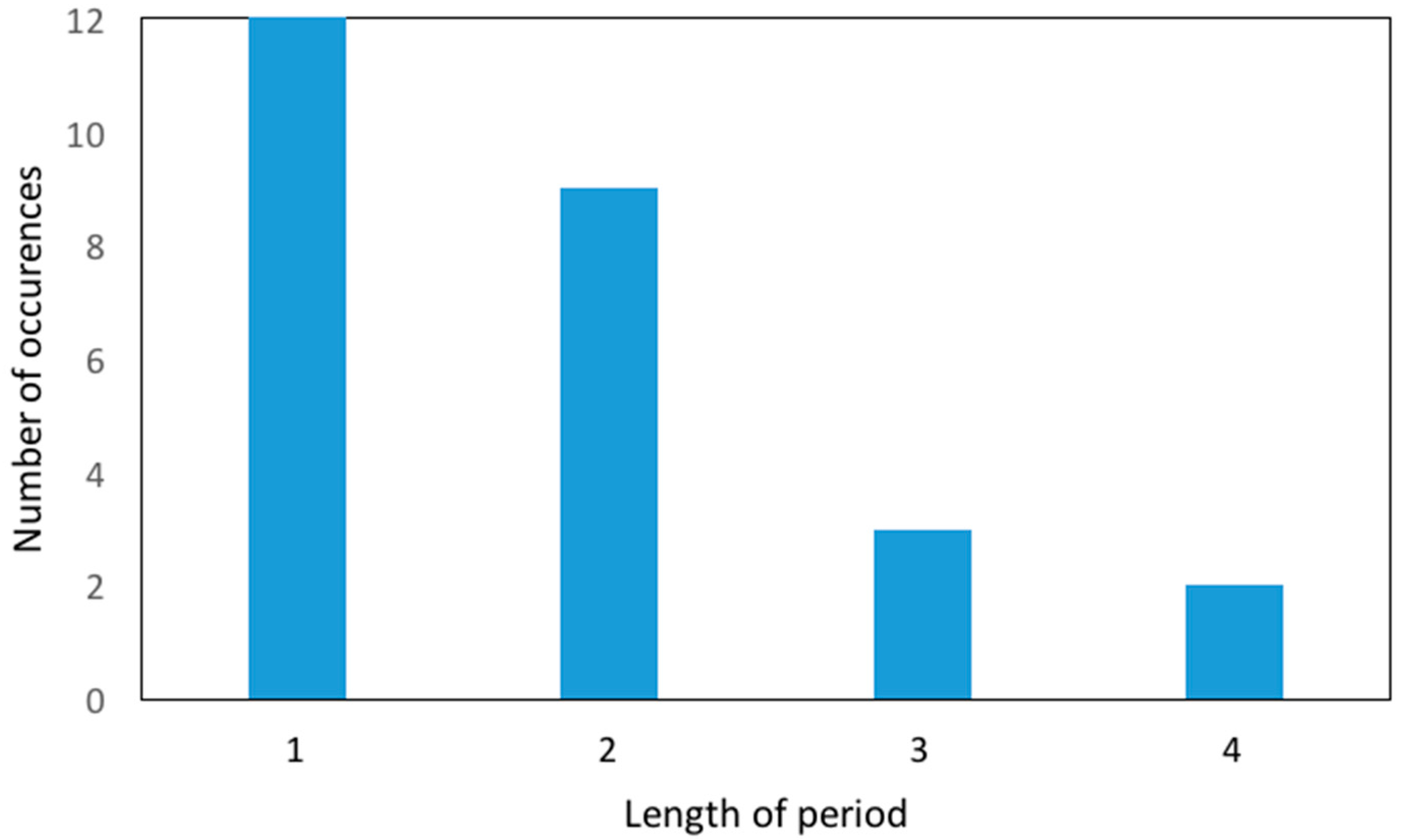
Figure 10.
True and estimated inflation rates.

Table 1.
Inflation data. All items index annual average (source: World Bank).
| 1961 | 1.7 | 1971 | 0.2 | 1981 | 8.8 |
| 1962 | 2.1 | 1972 | 3.2 | 1982 | 7.3 |
| 1963 | 2.1 | 1973 | 12.9 | 1983 | 4.4 |
| 1964 | 4.2 | 1974 | 16.9 | 1984 | 3.7 |
| 1965 | 1.9 | 1975 | 8.4 | 1985 | 10.9 |
| 1966 | 4.7 | 1976 | 10.1 | 1986 | 18.7 |
| 1967 | 10.7 | 1977 | 9.7 | 1987 | 53.4 |
| 1968 | 0.2 | 1978 | 8.8 | 1988 | 7.3 |
| 1969 | 11.3 | 1979 | 14.8 | 1989 | 0.8 |
| 1970 | 2.6 | 1980 | 14.1 | 1990 | 21.7 |
| 1991 | 26 | 2001 | 38.6 | 2011 | 17.7 |
| 1992 | 43.7 | 2002 | 15.5 | 2012 | 5 |
| 1993 | 143.5 | 2003 | 23 | 2013 | 2 |
| 1994 | 368.5 | 2004 | 10 | 2014 | 3.3 |
| 1995 | 235.6 | 2005 | 9.9 | 2015 | 6.9 |
| 1996 | −0.7 | 2006 | 11.3 | ||
| 1997 | 7.1 | 2007 | 6.4 | ||
| 1998 | 19 | 2008 | 14.7 | ||
| 1999 | 98.8 | 2009 | −0.2 | ||
| 2000 | 59.4 | 2010 | 6.9 |
Table 2.
Percentage changes in the median stamp price per year (sources: for the data until and including 12 November 1975, “Speciale catalogus 2002, Postzegels van Nederland en overzeese rijksdelen” NVPH, Amsterdam, Joh Enschede, and for the data since 25 November 1975, “Officiele postzegelcatalogus,” Suriname, 31ste Editie 2016, Guernsey, Uitgeverij Zonnebloem).
| 1961 | 33.33 | 1971 | 8.7 | 1981 | 50 |
| 1962 | −30 | 1972 | 20 | 1982 | −16.67 |
| 1963 | 0 | 1973 | 0 | 1983 | −50 |
| 1964 | 3.57 | 1974 | 0 | 1984 | 33.33 |
| 1965 | 3.45 | 1975 | 0 | 1985 | 10 |
| 1966 | 33.33 | 1976 | 16.67 | 1986 | −9.09 |
| 1967 | 25 | 1977 | 42.86 | 1987 | 120 |
| 1968 | 0 | 1978 | 0 | 1988 | 0 |
| 1969 | 0 | 1979 | −10 | 1989 | 0 |
| 1970 | −8 | 1980 | 33.33 | 1990 | 0 |
| 1991 | 0 | 2001 | −60 | 2011 | −12.5 |
| 1992 | 40.91 | 2002 | 70 | 2012 | 28.57 |
| 1993 | 30.65 | 2003 | −41.18 | 2013 | 13.89 |
| 1994 | 4220.99 | 2004 | −20 | 2014 | 7.32 |
| 1995 | 471.43 | 2005 | −43.75 | 2015 | 6.82 |
| 1996 | −61 | 2006 | 277.78 | ||
| 1997 | 15.38 | 2007 | 17.65 | ||
| 1998 | 61.11 | 2008 | 50 | ||
| 1999 | 148.28 | 2009 | 0 | ||
| 2000 | 177.78 | 2010 | 33.33 |
Table 3.
Estimation results for various regression models relating inflation with lagged inflation and current and lagged percentage changes in stamps prices. Estimated Newey-West adjusted standard errors are in parentheses.
Table 3.
Estimation results for various regression models relating inflation with lagged inflation and current and lagged percentage changes in stamps prices. Estimated Newey-West adjusted standard errors are in parentheses.
| Sample | Sample | Sample | |
|---|---|---|---|
| Variable | 1975–2015 | 1975–2015 (without 1993, 1999) | 1961–2015 (without 1993, 1999) |
| Intercept | 15.683 (5.398) | 11.032 (2.796) | 9.288 (2.171) |
| 0.026 (0.162) | |||
| 0.083 (0.005) | 0.085 (0.001) | 0.085 (0.001) | |
| 0.040 (0.013) | 0.043 (0.001) | 0.044 (0.001) | |
| R2 | 0.858 | 0.967 | 0.964 |
| p value tests | |||
| Normality | 0.000 | 0.131 | 0.000 |
| Autocorrelation | 0.010 | 0.037 | 0.008 |
Table 4.
Estimation results for the (unrestricted) MIDAS regression models, sample runs from 1975 to and including 2015. Estimated Newey-West adjusted standard errors are in parentheses. are the first-order differenced median stamps prices, where T again corresponds with years and q with the quarters 1, 2, 3, and 4, and differenced median stamps price. are the fourth-order differenced median stamps prices.
| Variable | Version 1 | Variable | Version 2 | ||
|---|---|---|---|---|---|
| Intercept | 1.828 | (3.240) | Intercept | 0.315 | (2.811) |
| 0.554 | (0.037) | 0.893 | (0.134) | ||
| 0.240 | (0.066) | 0.190 | (0.065) | ||
| 0.209 | (0.060) | 0.051 | (0.099) | ||
| 0.190 | (0.085) | −0.023 | (0.078) | ||
| 0.402 | (0.068) | 0.232 | (0.061) | ||
| 0.430 | (0.073) | 0.049 | (0.050) | ||
| 0.319 | (0.100) | 0.084 | (0.050) | ||
| −0.264 | (0.098) | ||||
| R2 | 0.932 | 0.944 | |||
| p value tests | |||||
| Normality | 0.184 | 0.645 | |||
| Autocorrelation | 0.149 | 0.740 | |||
| RMSPE, in sample | 19.305 | 18.363 | |||
Table 5.
Estimated historical episodes with high inflation.
| Years | Potential Causes |
|---|---|
| 1900s | Gold rush (Lawa railway construction) |
| 1930s | Economic decline, social upheaval in the form of riots |
| 1940s | WW II |
| 1957 | Establishment of the Central Bank of Suriname, Brokopondo-agreement with Alcoa and Eisenhower Recession |
Table 6.
Estimated parameters and associated standard errors in the EGARCH model.
| Parameters | Sample | |||
|---|---|---|---|---|
| 1961–2015 | 1873–2015 | |||
| μ | 1.457 | (0.200) | 1.595 | (0.219) |
| ρ | 0.327 | (0.089) | 0.314 | (0.096) |
| ω | −0.939 | (0.249) | −0.311 | (0.103) |
| 1.073 | (0.308) | 0.311 | (0.113) | |
| 0.711 | (0.182) | 0.208 | (0.095) | |
| 0.659 | (0.146) | 0.855 | (0.048) | |
© 2017 by the authors. Licensee MDPI, Basel, Switzerland. This article is an open access article distributed under the terms and conditions of the Creative Commons Attribution (CC BY) license (http://creativecommons.org/licenses/by/4.0/).
Share and Cite
MDPI and ACS Style
Franses, P.H.; Janssens, E. Recovering Historical Inflation Data from Postage Stamps Prices. J. Risk Financial Manag. 2017, 10, 21. https://doi.org/10.3390/jrfm10040021
AMA Style
Franses PH, Janssens E. Recovering Historical Inflation Data from Postage Stamps Prices. Journal of Risk and Financial Management. 2017; 10(4):21. https://doi.org/10.3390/jrfm10040021
Chicago/Turabian StyleFranses, Philip Hans, and Eva Janssens. 2017. "Recovering Historical Inflation Data from Postage Stamps Prices" Journal of Risk and Financial Management 10, no. 4: 21. https://doi.org/10.3390/jrfm10040021