Models of Investor Forecasting Behavior — Experimental Evidence


1
School of Mathematics, Georgia Institute of Technology, Atlanta, GA 30332, USA
2
School of Industrial and Systems Engineering, Georgia Institute of Technology, Atlanta, GA 30332, USA
*
Author to whom correspondence should be addressed.
J. Risk Financial Manag. 2018, 11(1), 3; https://doi.org/10.3390/jrfm11010003
Submission received: 1 November 2017
/
Revised: 15 December 2017
/
Accepted: 22 December 2017
/
Published: 28 December 2017
Abstract
:Different forecasting behaviors affect investors’ trading decisions and lead to qualitatively different asset price trajectories. It has been shown in the literature that the weights that investors place on observed asset price changes when forecasting future price changes, and the nature of their confidence when price changes are forecast, determine whether price bubbles, price crashes, and unpredictable price cycles occur. In this paper, we report the results of behavioral experiments involving multiple investors who participated in a market for a virtual asset. Our goal is to study investors’ forecast formation. We conducted three experimental sessions with different participants in each session. We fit different models of forecast formation to the observed data. There is strong evidence that the investors forecast future prices by extrapolating past price changes, even when they know the fundamental value of the asset exactly and the extrapolated forecasts differ significantly from the fundamental value. The rational expectations hypothesis seems inconsistent with the observed forecasts. The forecasting models of all participants that best fit the observed forecasting data were of the type that cause price bubbles and cycles in dynamical systems models, and price bubbles and cycles ended up occurring in all three sessions.
1. Introduction
Data and forecasting form the foundations of both long-term planning and operational control. In spite of the widespread use of computers and algorithms to assist with data processing and forecasting, human decision makers continue to affect forecasts in important ways, including the introduction of cognitive biases, strategic biases, and overconfidence into forecasts. For surveys of the impact of human decision makers on forecasts, see for example Armstrong (1985) and Ramnath et al. (2008). In this paper we focus on human forecasting behavior in a setting in which forecasters know the rational expectations value of the variable to be forecasted, and they also observe data of the variable to be forecasted, where the individual data values are allowed to deviate from the rational expectations value. We conducted experiments in which the participants were asked to forecast future prices, in which the actual prices were endogenous to the experiment through the trading decisions of the participants, and in which the rational expectations value of future prices (fundamental value of the traded asset) was clear and known to all the participants. One question is whether such participants place more emphasis on the rational expectations value or on the observed data to make their forecasts.
If investors’ forecasts were consistent with the rational expectations hypothesis, then the volatility in forecasts and prices would be caused by “external” surprises and not by the “internal” forecasting behavior itself, and the forecasts and resulting prices would be less volatile than the earnings produced by the assets. However, Shiller (1981a, 1981b); LeRoy and Porter (1981); and later Campbell and Shiller (1987, 1988); Shiller (1986); West (1988a, 1988b); and LeRoy (1989), presented empirical evidence that stock prices are typically much more volatile than the earnings produced by the stocks. Thus empirical evidence indicates that the rational expectations hypothesis does not provide an accurate model of investor forecasts and asset prices. Hence we are interested in studying alternative models of forecasting behavior.
Models of boundedly rational forecasting behavior have shown that small changes in investors’ forecasting behavior can qualitatively change price trajectories. For example, Cheriyan and Kleywegt (2016) showed that a small change in the weight that investors’ forecasts place on recent data relative to older data can change price trajectories from convergent trajectories to cyclical trajectories consisting of repeated bubbles and crashes, and the instability is affected by investors’ overconfidence in the information contained in observed price data. Also, it was shown that if investors’ forecasts exhibit behavior called panic, then the price cycles can become unpredictable. Thus, an understanding of forecasting behavior contributes to an understanding of the qualitative behavior of price trajectories.
Therefore, our interest in investor forecasting behavior lead us to the following questions: Are there simple models that can describe investors’ forecasts accurately? How accurately does the rational expectations hypothesis describe investors’ forecasts? What does observed forecasting behavior imply regarding the resulting behavior of price trajectories, that is, whether price trajectories converge, or predictable price cycles occur, or trajectories are unpredictable? Questions such as these have been asked by both researchers as well as policy makers who are interested in studying, and sometimes containing or controlling, asset price dynamics.
In this paper, we report experiments conducted to study investor forecasting behavior. We designed a market for a virtual asset in which the experimental investors report their price forecasts to the experimenter, and enter their buy and sell orders in the market, repeatedly over time. The market clearing prices are determined by the investors’ buy and sell orders, and are therefore endogenous, and the market clearing prices are reported to the investors in real time. Before each experimental session, the investors were reminded of the theory of the fundamental value of an asset, and they were told how the earnings of the asset would be determined and what the resulting fundamental value of the asset was. Nevertheless, the resulting price trajectories exhibited cycles. We calibrated and compared various models of investor forecast formation. The experimental results indicate that:
- The rational expectations hypothesis does not provide an accurate model of investor forecasting behavior, even when the earnings rate and fundamental value of the asset are known with certainty by investors.
- A simple one-parameter exponential smoothing model of investor forecasting behavior is remarkably accurate. Models with a larger number of parameters provide only a slightly better fit.
- There is strong evidence of investor overconfidence in the information content of observed price data. In the experiment, the fundamental value of the asset was known to the investors and therefore the observed prices contained no additional information regarding the fundamental value of the asset. Nevertheless, investor forecasts relied mostly on observed price data.
- Except for a few experimental investors, the price forecasts were increasing in the extrapolated prices. That is, most experimental investors did not exhibit evidence of panic, as defined in Cheriyan and Kleywegt (2016), in their forecasts.
Definition of Key Terms
A typical experimental setting consists of a number of participants buying and selling units of a virtual asset with virtual currency in a market. Usually, the participants can buy and sell assets. In some experiments, the participants can also be forecasters who only generate forecasts and do not trade.
A virtual asset market implements a specified trading mechanism for trading units of a virtual asset and virtual currency. All virtual asset markets have a finite duration. The fundamental value of the asset may be specified exogenously or it can be computed from the dividend payoffs. The asset may provide either periodic dividends, or only a terminal dividend. Also, it may or may not have a salvage value.
An experiment consists of one or more sessions. A session involves a group of participants participating in the asset market. Each session consists of one or more trading runs. Two or more trading runs with common participants are called repeated markets by some authors. At the beginning of each trading run, the investors are given an initial endowment of virtual currency and units of the virtual asset. The investors use the trading mechanism to participate in trades. At the end of the trading run, the participants are rewarded, typically as a function of their final portfolio of virtual currency earned and virtual asset in possession. In some experiments, there is also a reward associated with forecast accuracy.
The trading mechanism can be a continuous-time trading mechanism such as a double-auction, or a discrete-time trading mechanism such as a call market mechanism. For a market with a discrete-time trading mechanism, the trading run is divided into multiple (trading) periods. During a period, traders enter buy and sell orders. At the end of the trading period, the price of the asset is determined by market clearing and the trades are executed based on the market clearing price. For a market with a continuous-time trading mechanism, the trading run consists of only one trading period. For example, in a double auction market, the traders may post buy and sell offers, or accept existing open offers resulting in trade; in this case the instantaneous price varies throughout the trading period.
Note that in our experiments, the object of interest is investor price forecast formation when both knowledge of the fundamental value of the asset as well as price data are available to the investor. As a result, each participant’s forecast in each trading period in each session constitutes an observation. Thus, over the three experimental sessions that we conducted we collected 2760 observations.
2. Models of Price Forecast Formation and Literature Review
In this section, we briefly review some models of asset price forecasts and the resulting market clearing prices. We also review the related literature.
Time is indexed by . Each unit of asset pays a dividend at time t. Let denote the price of the asset at time t before the dividend is paid. Let denote the modeled investor forecast at time t of the price at time . Suppose that the investors in the market are indifferent between investing and not investing in the asset if they expect a rate of return of , that does not depend on time. In each time period, investors can rebalance their portfolios without transaction cost, and they forecast only one period into the future. Then the indifference price at time t is
For extensions of this model and an estimation procedure for the expected rate of return see Wong and Chan (2004).
In the experimental sessions that we conducted, the dividend process was revealed to everyone, enabling the participants to compute explicitly. Note that, given , it holds that each specification of a model to compute forecasts , and appropriate initial conditions, defines a unique discrete time dynamical system of the asset price process through Equation (1). This way, a model of forecast behavior has direct implications regarding the resulting asset price dynamics. Cheriyan and Kleywegt (2016) studied models of asset price dynamical systems, and showed how the qualitative behavior (convergence, cycling, or unpredictable “chaotic” behavior of price trajectories) of these systems depend on the properties of the price forecast process. In this paper we report the properties of the price forecast processes observed in our experiments, and in Section 5 we comment on the implications of the forecasting behavior observed in the experiments for the asset price dynamics.
Next we review some models of asset price forecasts. For the fundamentalist investor, the price forecast is simply the fundamental value
assuming that the infinite sum is convergent. (That is, the expected growth rate of the forecasted dividends is less than .) In our experiments, , and can be computed explicitly from the given dividend process and the salvage value of the stock. These computations are given in Appendix A.
Price forecasts may also be influenced by observed historical price data, especially recent price data. Different assumptions about how past price data affect price forecasts give rise to different models for forecast formation.
2.1. Extrapolation-Correction Models of Forecast Formation
It is convenient to consider the prices and forecasts scaled by the fundamental value, as follows:
Let denote the growth rate of scaled prices in period t, that is,
2.1.1. Extrapolated Price
The extrapolation forecast of the price growth rate is given by
where is an appropriate initial value. Thus, the extrapolation forecast is an exponential smoothing forecast. Note that corresponds to the weight that the investor gives to the most recent price ratio. If the forecaster used only the extrapolation forecast, then the corresponding scaled forecast for the price at time would be
Note that at time t, are known to the investor, but the price has not yet been observed.
2.1.2. Price Forecast
We also consider price forecasts that are functions H of the extrapolation forecast and the fundamental value. Although the price forecast depends on both the extrapolation forecast and the fundamental value, it is convenient to use notation that shows only the scaled extrapolation forecast as an argument of H. Thus, the scaled price forecast is given by
where is a function that captures some forecast behavioral characteristics of the investor. A fairly general class of functions H are included. The only property that we require is that
That is, if the extrapolation forecast is equal to the fundamental value, then the price forecast should also be equal to the fundamental value. As an example, corresponds to rational expectations, while corresponds to extrapolation-only price forecast.
One may expect H to be nondecreasing in a neighborhood of , that is, the price forecast increases with the extrapolation forecast if the extrapolation forecast is close to the fundamental value. For larger values of , H may increase, perhaps at a decreasing rate. Alternatively, H may increase and then decrease, in which case we say that the investor exhibits panicking behavior. This corresponds to the investor losing confidence in the extrapolation forecast and adjusting the price forecast closer to the fundamental value. Such functions H will be called non-mononotic.
2.2. Linear Model of Forecast Formation
As a benchmark to compare our results, we also consider a simple linear model of forecast formation. According to this model, the price forecast for next period, , is given by
where is the fundamental value at time t, and and are parameters. Thus, the forecasts are linear functions of the deviations of the past price from the fundamental value. This model was first introduced in Brock and Hommes (1997) where the resulting price dynamics are studied.
2.3. Literature Review
The literature specifically on investors’ price forecast behavior is very small. At the same time, several researchers such as Smith et al. (1988) have conducted experiments to study behaviors that may result in asset price bubbles, and the subsequent literature on such topics is relatively large. Therefore, here we review experimental work that study not only price forecast behavior, but also the related asset price formation. We classify the experiments in this area based on the following properties: purpose of the experimental work, endogeneity of supply and demand, finiteness of the time horizon, market mechanism, and reward mechanism.
2.3.1. Purpose of the Experiments
The primary purpose of our experiments was to learn about investors’ price forecasting behavior when asset prices are observed in each period, and the fundamental value of the asset is known. For that reason we collected investors’ price forecasts during the experiments, so that various models of investor forecast formation could be calibrated and compared. The secondary purpose of our experiments was to determine which of the qualitative regimes of asset price trajectories identified in dynamical systems models (convergence of asset prices, cycling of asset prices, or unpredictable asset price trajectories) the observed forecasting behavior corresponds to. We conducted these experiments in an experimental market setting, so that we also observed the price trajectories that resulted from the participants’ forecasts and trading decisions.
Similar to this paper, some of the experimental studies addressed belief or expectation formation among participants. For example, Nickerson et al. (2007) explicitly captured participants’ price expectations for future periods and concluded that participants’ beliefs converged to the fundamental value only after observed prices converged. Hirota and Sunder (2007) studied the effect of first and higher-order beliefs by designing experiments with a publicly announced range of dividends that was wider than the privately communicated actual range of dividends.
Many of the experimental studies focused on convergence of asset prices to the theoretical fundamental value. For example, Ball and Holt (1998) compared the prices resulting from trading with the fundamental value. Some researchers such as Nickerson et al. (2007) studied price bubbles in repeated markets with the same set of participants.
There were also other specialized objectives to some of these studies. Hirota and Sunder (2007) studied the effect of investors’ decision horizons on the presence of bubbles and they found that shorter decision horizons (compared with the maturity of the asset) can lead to larger bubbles. Lugovskyy et al. (2009) studied the effect of the tâtonnement trading institution on price bubbles and concluded that the participants were able to learn about supply and demand during the tâtonnement process, thereby reducing price bubbles.
2.3.2. Exogenous and Endogenous Supply and Demand
The supply and demand of the asset are exogenously specified in experiments that study the effectiveness of market mechanisms in facilitating the convergence of prices to the equilibrium price. In such a setup, in each trading period some of the participants are given the role of buyers and the rest are given the role of sellers. Each buyer and seller is given an initial endowment of currency or the asset, respectively. Moreover, the value of the asset for each buyer and seller is specified privately to the buyer and seller. Thus, there are a priori supply and demand curves and a market clearing price in each trading run. Different market mechanisms, such as the double auction mechanism, are used to generate a price trajectory for the asset and this price trajectory is compared with the market clearing price. For example, Ball and Holt (1998); Smith et al. (1988) conducted such studies.
Most of the experiments related to our work use endogenous supply and demand (Camerer and Weigelt 1993; Hirota and Sunder 2007; Lugovskyy et al. 2009; Nickerson et al. 2007). In this setup, at the beginning of a trading run, every participant is given an initial endowment. Thereafter, in each period, each participant can enter buy and sell orders. Presumably, they make these decisions by taking into account the market clearing prices, their own forecasts of the future prices, as well as the revenue stream associated with owning the asset. Thus, in each period the supply and demand of the asset are endogenous to the experimental market. Our experimental setup also follows this endogenous supply and demand approach.
2.3.3. Finite Time Horizon and Learning
Many of the experiments reported in the literature have a pre-announced number of periods in each trading run. For example, both Nickerson et al. (2007) and Lugovskyy et al. (2009) used trading runs consisting of 15 periods each.
In many experiments the asset is worthless at the end of the trading run. For example, Nickerson et al. (2007) and Lugovskyy et al. (2009) considered an asset that paid a fixed expected dividend d at the end of each period and that had no salvage value. Assuming no discounting, the fundamental value of the asset at the beginning of period t was . Thus, the fundamental value decreased linearly throughout the trading run and the participants knew ex ante that the asset would be worthless at the end of the trading run. Consequently, prices fell towards the end of the trading run. Since the dividend process was pre-announced, the participants could anticipate this price trajectory. In repeated markets as in Nickerson et al. (2007), one reasonable estimator of when the price process peaks was the peak time period in the previous trading run. Consequently, in each successive trading run the peak occurred earlier than in the previous trading run, and as a result the size of the bubble decreased because the fundamental value was also larger in earlier periods. This observation lead to the conclusion that learning caused the bubbles to disappear.
One question that arises naturally is what happens when investors do not have the opportunity to form expectations using backward induction—e.g., reasoning such as “if it is certain that the price is 0 at the end of period 15, it may not be very high at the end of period 14”. Hirota and Sunder (2007) considered a setup which made such backward induction difficult. In their setup, the asset paid a known terminal dividend only at maturity (at the end of 15 or 30 trading periods). In some trading runs, it was known in advance that the duration would be 15 periods and that the asset would mature at the end of 15 periods; in this setting, backward induction was possible. In other trading runs, the asset matured at the end of 30 periods; however the participants were told that the experiment would end at an unknown time most probably much earlier than the life of the asset. If the trading run lasted for 30 periods, then they would receive the known dividend, otherwise they would receive a payout of the average price forecast for the asset when the trading run ends. In this setting, the apparently random end of the trading run removed the anchor that the terminal dividend provided for backward induction. Their results suggest that the latter setup is more conducive to formation of asset price bubbles.
Another approach to eliminate backward induction is to make the number of periods in the trading run random. In this kind of probabilistic stopping, in each period the trading run ends with a pre-specified probability. It can be shown that for an asset paying constant dividends, the fundamental value under probabilistic stopping with probability p is equal to the fundamental value under an infinitely-long trading run with discount factor of (see Lemma 1). Camerer and Weigelt (1993) used trading runs with probabilistic stopping to study convergence of prices to fundamental value and to test if prices are rational forecasts of the fundamental value. Ball and Holt (1998) used a variation of this in which each individual asset can expire with a pre-specified probability. However, in their experiment the total length of the trading run was pre-announced (10 periods), thus the probabilistic stopping only created an effective discounting but did not eliminate the end of horizon effect.
In the current work, we use probabilistic stopping; in each period the trading run can end with a pre-announced stopping probability similar to Camerer and Weigelt (1993). Thus the participants cannot use backward induction to value the assets. Moreover, we pre-announced the total duration of the experimental sessions to be about three and a half hours, which is atypical in this literature. Our reasoning was that even with probabilistic stopping, towards the end of the time allowed for the session, the participants might reason that even if the trading run did not end, the session would end soon; in such a setting they might want to apply thinking analogous to backward-induction and offer to sell their assets for decreasing prices. A pre-announced long duration for the experimental sessions helps to reduce the effect of such thinking if the trading runs end well before the time that the participants thought that the session might end.
2.3.4. Market Mechanism
Depending on the objectives of their studies, different researchers use different market mechanisms. For example, Ball and Holt (1998); Camerer and Weigelt (1993); Hirota and Sunder (2007) used a continuous double auction mechanism. In this mechanism, participants announced their bids and asks; at any time any participant could accept a bid or an ask, and the price associated was recorded as the current transaction price. In these studies, the average of the transaction prices was used as a proxy for the market clearing price for that period. On the other hand, researchers such as Nickerson et al. (2007) used a call market mechanism. In this mechanism, in each trading period, each participant entered buy and/or sell orders. At the end of the period, all orders were aggregated into market supply and demand curves. An equilibrium price was determined that cleared the market. All feasible trades (bids above the equilibrium price, asks below the equilibrium price) were executed. Bids and asks at the equilibrium price might be only partially executed (in which case, some tie breaking or apportioning mechanism was used). Other authors have used other market mechanisms. For example, Lugovskyy et al. (2009) used the tâtonnement mechanism. In this mechanism, in each period the market maker announced a suggested price and the participants placed their tentative buy and sell orders at that price. If the aggregate supply equaled the aggregate demand then the suggested price became the market clearing price and all trades were executed; otherwise, the market maker announced an updated suggested price and the participants again placed their buy and sell orders at the new suggested price. The process repeated until the market cleared or a particular exit criterion was met (e.g., if the number of iterations reached a maximum).
In our setup, we use a slight modification of the call market mechanism. In each period, each participant can place multiple buy and sell orders, effectively specifying their individual supply and demand curves. These are aggregated into market supply and demand curves. Their intersection determines the market clearing price. Trades are executed at the market clearing price—all buy orders above the market clearing price and all sell orders below the market clearing price are fully executed. Orders at the market clearing price are filled completely if the aggregate supply and demand match exactly; in general, the maximum number of orders at the market clearing price are filled, and they are filled in the temporal sequence in which the orders were entered (i.e., on a first-come first-served basis). Some orders can be partially filled.
We chose to use this market clearing mechanism primarily to make sure that each period results in a unique equilibrium price. The prices in prior periods are common knowledge to all participants, and we hypothesize that the participants use this information to form price forecasts.
2.3.5. Reward Mechanism
The reward mechanisms found in the literature are quite varied. Most experiments pay a combination of a fixed participation fee and a reward proportional to the participant’s performance in the experiment. The participant’s performance is evaluated based on factors such as the total virtual wealth at the end of the experiment and the forecast accuracy (if the experiment collected forecast data). For example, in Hirota and Sunder (2007) participants who were price predictors were paid based on the accuracy of their predicted prices; in Nickerson et al. (2007) the participants also received payments for accurate predictions. Some researchers used a fixed exchange rate (i.e., a pre-announced virtual currency to real currency exchange rate), a pre-announced payment schedule (e.g., for accuracy of predictions), or they divided a pot of money in proportion to the total virtual wealth at the end of the experiment, as in Hirota and Sunder (2007) for the participants who were investors. Ball and Holt (1998) argued against rewarding only the participant with the highest earnings as it may induce indifference or extreme risk seeking in people who are relatively behind in terms of their earnings.
In our experiment, rather than provide a fixed participation fee to each participant, three prizes were awarded at the end of each experimental session. Two of these were a function of their total wealth at the end of the experiment and one was for the best forecast accuracy. The details and rationale for these prizes are given in Section 3.4.
3. Design of the Behavioral Experiment
Our experiment consisted of three sessions of a virtual asset market with a discrete-time trading mechanism, as given in Process Flow 1.
| Process Flow 1 Process flow for an asset market with a discrete-time trading mechanism. |
|
3.1. Approaches to Reduce End of Horizon Effect
In most market experiments the asset becomes worthless at the end of the last period. Therefore, if the total number of periods in the trading run is known in advance, the asset price decreases to zero towards the end of the trading run. If there are repeated trading runs in an experimental session, the decreasing trend of prices during a trading run eventually reduces the occurrence of price bubbles in the later trading runs.
To alleviate this effect caused by a known time horizon, we used probabilistic stopping. At the end of each period the trading run can end with a stopping probability . Thus, the total number of periods in each trading run is a geometric random variable. This was explained to all participants, including the value of the stopping probability, in advance of each trading run.
Unlike traditional classroom experiments that last 1 or 2 h, we set up our sessions to last for three and a half to four hours. Thus, at least during the initial part of the session, the participants did not consider the end of the session when making their trading decisions.
We also instituted a salvage value of 100 Experimental Currency Units (ECUs) for each unit of asset held when the trading run ended. Theoretically, this just adds a constant to the fundamental value of the asset. We decided to add the salvage value after an initial trial run of the experiment (the data from the trial run were not used) to reduce the fixation of some participants on the possibility that the asset may become worthless at any time.
3.2. Dividend Structure
In each period, a dividend was paid for each unit of asset held. The dividend was added to the cash-on-hand of each participant.
For the first two sessions, the dividend was fixed to 10 ECUs per unit of asset in each period. For the third session, the dividends were the same for all participants but were random for each period. In each period the market was in a state . The state transition followed a discrete time Markov chain with the transition matrix
The initial state, , was chosen at random with equal probability. The dividend for each period had a distribution depending on as given in Table 1.
3.3. Experimental Sessions
The experiment consisted of three sessions, each with a new group of participants. Each session lasted for about four hours in total and consisted of an overview, training trading run, actual trading runs, and post-session debriefing.
The overview included an explanation of the Process Flow 1, probabilistic stopping of trading runs including the memoryless property of the geometric distribution, the dividend process, the concept of fundamental value and its calculation, the process for placing buy and sell orders, and the market clearing process to determine the market clearing price and market clearing trades. (All participants were masters students in the Quantitative and Computational Finance program or Ph.D. students, and the explanation of fundamental value was a review of a concept already familiar to them.) The stopping probability for all trading runs was and this was announced to the participants.
The training trading run lasted four periods. The purpose of the training trading run was to familiarize the participants with the market simulation software, by entering forecasts, placing buy and sell orders, and answering questions that tested their understanding of the experiment. It was made clear that the number of periods was fixed only for the training trading run. The earnings in the training trading run were not taken into account for the determination of the eventual compensation.
After the training trading run, it was announced that a real trading run was about to start and that the total number of periods would be random as explained. The experiment started with a number of questions for each participant to test participants’ understanding of the experiment. Each participant was endowed with an initial portfolio of 5000 Experimental Currency Units (ECUs) and 50 units of the virtual asset.
Thereafter, period 1 started. In each period each participant was shown a screen displaying the participant’s current cash and asset balance, a chart of the previous prices and a table of previous prices, the dividend history, and previously executed buy and sell orders for the participant, input boxes to answer questions described below, an input box to enter the participant’s price forecast, and input boxes to enter buy and sell orders. For the third session with Markov dividends, additional information was displayed as described in the next section.
In each period each participant had to enter answers to the following questions:
- The expected number of time periods remaining in the trading run.
- The expected total dividends paid by one unit of asset from the current period until the end of the trading run.
- The total of the expected dividend from the current period until the end of the trading run and the salvage value for one unit of asset held until the end of the trading run.
- The participant’s forecast of the price per unit of asset.
- The current state of the market (only session 3—Markov dividend case).
After they entered the feedback and forecast information, the order entry portion of the screen was enabled and they could enter multiple buy or sell orders. Participants could also not trade in a period, however, the software design enforced that there would be at least one order entered among all participants in every period. This was required to ensure that there is an equilibrium price in every period.
Once a participant made her entries, a wait screen was displayed. After all participants made their entries, the market was cleared based on the orders and the new equilibrium price was determined.
Subsequent periods followed the same pattern until the computer determined that the trading run was over.
At the end of the trading run, the participants’ portfolios were converted into virtual currency. Then, the winners were determined and were announced.
Finally, there was a short debrief session where we gathered feedback from the participants about the session.
The specific details of the experimental sessions are given in Table 2.
3.4. Incentive Mechanism
Rather than provide a fixed participation fee to each participant, three prizes were awarded at the end of each experimental session.
- Two randomly selected players split $300 in proportion to the value of their final amount of virtual currency, after payment of the salvage value.
- The participant with the largest final amount of virtual currency received a prize of $100.
- The participant with the smallest mean square forecast error received a prize of $100.
The motivation for this incentive scheme is as follows. Other behavioral experiments have shown that people are more willing to perform a task when either it has no remuneration (i.e., it is considered to be a help) or when the remuneration is significantly large. In our case, $18.75 (= $300/16) would not have been a lucrative enough participation fee for four hours’ time. On the other hand, splitting the $300 among two randomly selected participants makes the incentive more lucrative. This is supported by the framing effect and pseudocertainty effect reported by Kahneman and Tversky (Tversky and Kahneman (1974)) wherein when evaluating such conditional situations, people evaluate the options assuming that the selection process has already happened. Thus, in our case, the participants would be looking at an amount of the order of $150, which is lucrative. Also, random selection of two participants helped avoid participants dropping out of the experiment if they are doing poorly.
The prize for the largest portfolio incentivized playing the game strategically and thoughtfully and the prize for the smallest forecast error incentivized careful forecasting and reporting of forecasts.
Our incentive structure is somewhat unconventional. Our incentive structure is such that the risk faced by a participant who invests in the virtual “risky” asset is not the same as the risk that an investor would have faced if the market were real and the investor invested in an asset with the same dividends. Of course, the risk faced by a participant who invests in the virtual risky asset affects the price that the participant is willing to virtually pay for the asset during an experiment. Also, rewarding the participant with the largest virtual wealth at the end of a session disproportionately creates tournament incentives that may also affect the price that the participant is willing to virtually pay for the asset during an experiment. When making these observations, it is important to keep in mind that the purpose of the study was to model investor forecast formation and not price formation in a market.
3.5. Participant Demographics
The participants were students belonging to the Ph.D. (ISyE, Math) and Masters (Quantitative and Computational Finance—QCF) programs. We chose to include only Masters or Ph.D. students to ensure that they had sufficient background knowledge of basic probability. Basics of asset valuation, discounted cash flow, and the memoryless property of the geometric distribution were explained to all the participants during the overview session.
All subjects gave their informed consent for inclusion before they participated in the study. The study was conducted in accordance with the Declaration of Helsinki, and the protocol was approved by Georgia Tech’s Institutional Review Board (Protocol H11292, Approved on 07 October 2011).
4. Results
This section provides the descriptive summary of the sessions and the computational results.
4.1. Summary of Observations
Though the first session had two trading runs, the second trading run did not complete within the time allotted for that session. So we used only the completed trading run for data fitting. There was only one trading run per session for the remaining two sessions. Therefore, from here on we will use the terms session and trading run interchangeably.
4.1.1. Equilibrium Price
Since in each period, the trading run could end with a stopping probability of , the number of time periods T was Geometric with parameter . The expected total returns for one unit of stock can be computed as
where is the dividend at period t. For sessions 1 and 2, the fundamental value was constant throughout and equaled 600 ECUs. For session 3, the computation of fundamental value is given in Appendix A. For session 3, the fundamental value at the beginning of the trading run was also 600 ECUs.
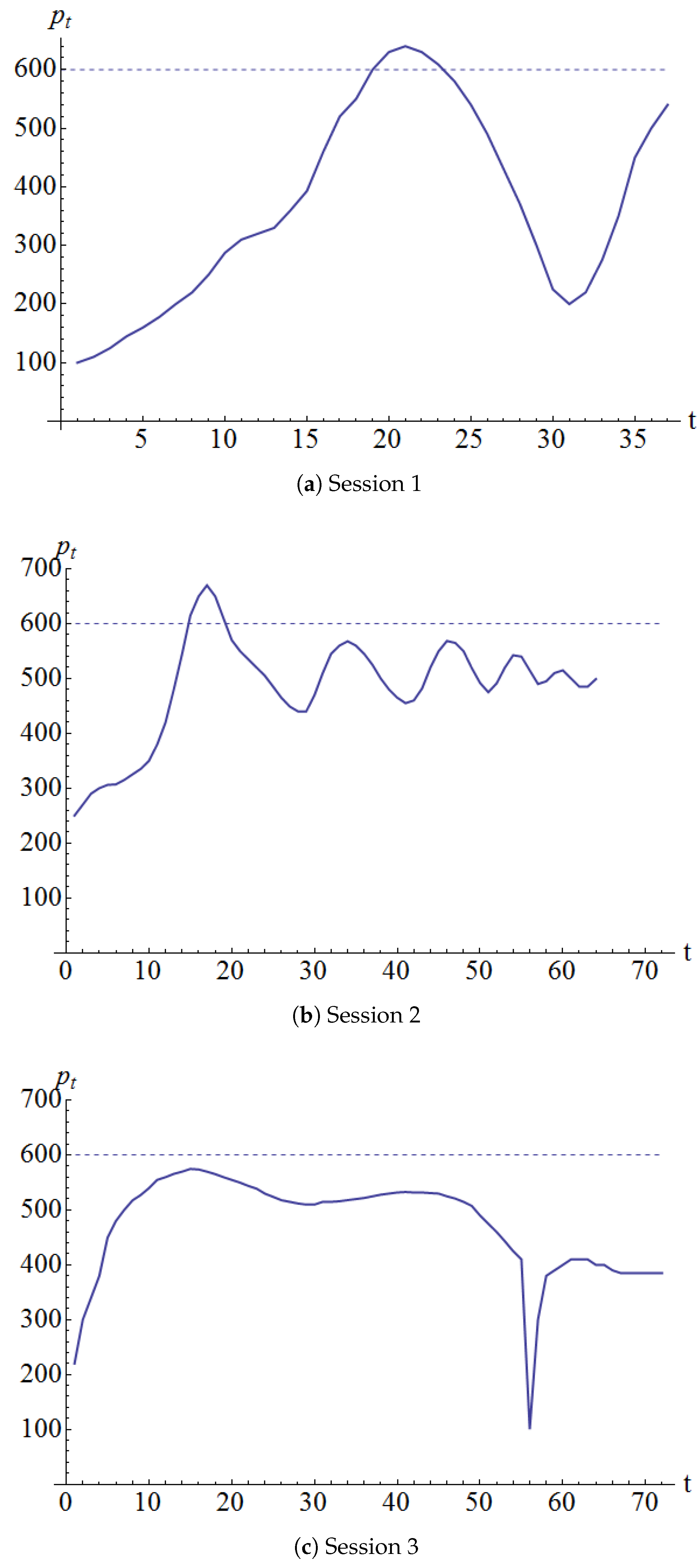
Figure 1 shows the realized equilibrium prices for the three sessions. Sessions 1 and 2 had prominent price cycles whereas session 3 had milder price cycles.
In all three sessions, the prices started from well below the fundamental value and started increasing thereafter. This phenomenon was observed in many other market experiments, see for example (Camerer and Weigelt (1993); Nickerson et al. (2007)).
In the third experimental session, there was a sudden downward spike in period 56. It was revealed to have been caused by one participant who panicked for some unknown reason and wanted to get rid of all his assets. So he offered to sell them for 0.01 ECU each. The market rebounded the very next period. (The data from this spike onwards were excluded from the calculations that follow.)
From the graphs of the price process, it appears that the participants had a perceived value that was lower than the fundamental value of 600 ECUs. In other words, they seemed to have made most buy-sell decisions as if the fundamental value was somehow smaller than the true fundamental value.
4.1.2. Price Forecasts
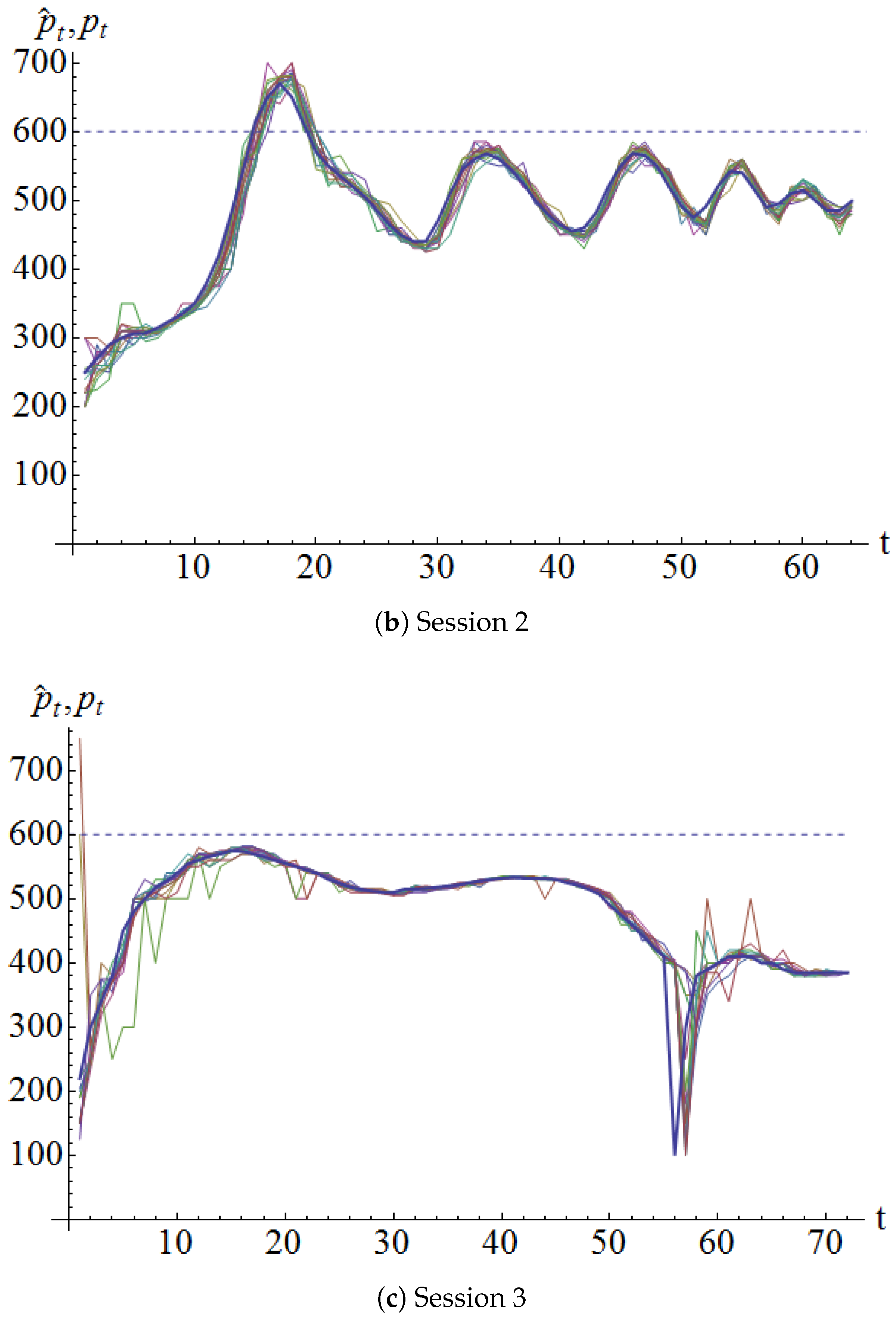
In each period, each participant was required to enter a price forecast for that period. Recall that the market clearing price in a period was determined only after the buy and sell orders were processed. Figure 2 shows a plot of the price forecasts for each session by each participant along with the market clearing price (solid line). It can be seen that the price forecasts usually followed the market clearing price.
The forecasts in the initial few periods are interesting. It seems that some of the participants started with a near-rational forecast and adjusted them down as the trading run progressed. On the other hand, some “skeptics” started with a very low forecast and adjusted them upwards as the trading run progressed.
4.1.3. Earning Forecasts
As part of the initial survey, each participant was asked the following question:
Given the compensation rules and the number of participants, how much money do you think you will earn in this experiment?
Table 3 summarizes the responses. In every session, the average of the participants’ expected earnings was at least twice the average prize money per participant for that session. Though there were some participants who expected to earn less than this average, a majority of them reported a higher than average earnings. Perhaps, this suggests an individual belief that they are better than the rest. This observation is reminiscent of the investor overconfidence mentioned in literature (e.g., Chuang and Lee (2006); Scheinkman and Xiong (2003)).
4.2. Comparison of Models Fitted with Data
4.2.1. Data Used
The data used for model calibration are the equilibrium prices and the participants’ forecasts from the three sessions.
First, we cleaned the data by fixing obvious typographical errors. Typically, the error was omission of the decimal point.
In the initial few periods of each of the three sessions, the equilibrium price increased from a value much lower than the fundamental value. A possible explanation is that the participants were trying to learn how the rest of the participants would behave. However, the models that we wanted to fit with the data were not intended to capture such initial learning or adaptation. Consequently, we used a subset of the data when the initial effect had passed. Moreover, we wanted to choose a subset of the data in a way that is endogenous to the data itself and not dependent on the model that we fit. To achieve this, we used the following approach: In the equilibrium price chart, let be the price in the first price trough. We discarded the data from the initial periods during which the price was smaller than . According to this approach, the number of dropped periods for the three sessions was between 7 and 11. Finally, to use the same number for all three sessions, we simply discarded the data from the first 10 periods in each session.
We also checked this approach using the calibrated models with the quadratic H function given in Section 4.2.8. We calibrated a sequence of models by successively dropping more initial periods from the data set. We observed that the fitted parameter values stabilized by the time we dropped the first 10 periods’ data.
In addition, for session 3, we dropped the data from period 56 onwards. This was done to avoid the effects of the spike that occurred in period 56.
4.2.2. Parameter Estimation Method
Parameter estimation was done by least squares fitting. We use the following notation.
(, as discussed above.)
Consider a family of models of forecast formation represented as
where denotes the vector of parameters of the model and are i.i.d. random variables.
The parameter fit for participant u in session is given by
The parameter fit using all data in all sessions is given by
To compare the different models that were fitted, we use the Leave-One-Out-Cross-Validation (LOOCV) approach. According to this approach, the observations in the data set are partitioned into subsets. The model is fitted using all but one subset, and then the fitted model is used to calculate forecasts for the omitted subset. The forecast error is recorded. This step is repeated with each subset of the data set left out in turn. Then the root mean square error (RMSE) of all the recorded forecast errors is calculated. The LOOCV RMSE of different models are compared. We perform the LOOCV validation with two types of subsets: (1) leave-one-period-out LOOCV, in which each period’s data for each participant is a subset; and (2) leave-one-session-out LOOCV, in which each session’s data is a subset. For details of this method, please see Appendix B.
4.2.3. Comparison of Fitted Models
We fit various models with the data. The individual models are covered in subsequent sections; the key parameters of these models are given in Table 4.
The model is the pure rational expectations model—according to the rational expectations model, the participant’s forecast equals the fundamental value (also recall that the participants were told the fundamental value in each period). Note that model BASE has no parameters to be fitted. Next we consider two one-parameter models. The model F is a “modified rational expectations” model where the hypothesis is that the participants believe that the fundamental value is some number other than the fundamental value communicated to them, and they forecast their belief of the fundamental value. Model assumes that the investors use only simple exponential smoothing and therefore has only one parameter. Model has 2 parameters, and is based on Brock and Hommes (1998). Models and belong to the family of extrapolation-correction models proposed in Cheriyan and Kleywegt (2016), with 3 and 4 parameters respectively.
4.2.4. Rational Base Case
For comparison, we take as base case the rational expectations forecast of a fully informed participant (BASE). That is
Thus, there are no parameters to fit for this model. For the Markov case in session 3, we used the reference fundamental value of 600 to fit the model.
Table 5 gives the leave-one-period-out LOOCV RMSE for each session.
Also, the leave-one-session-out LOOCV RMSE is
4.2.5. Modified Rational Expectations
Model F is similar to BASE, except that a parameter representing “perceived fundamental value” is now fitted with data.
where is the parameter to be fitted.
Table 6 gives the leave-one-period-out LOOCV RMSE for each session.
The leave-one-session-out LOOCV RMSE is given by
4.2.6. Simple Exponential Smoothing
Model ES uses simple exponential smoothing with initial price ratio of 1.
Table 7 gives the leave-one-period-out LOOCV RMSE for each session.
The leave-one-session-out LOOCV RMSE is given by
4.2.7. Brock and Hommes Model (BH)
Note that the forecast in period is a linear function of the price in period . However, in our experiment, at the beginning of period t, the participants entered the price forecast for that period. Therefore, we modify the BH model to
Table 8 gives the leave-one-period-out LOOCV RMSE for each session.
The leave-one-session-out RMSE is
4.2.8. Exponential Smoothing with Quadratic H (ESH2)
The correction function is given by
In this case, the model function is given by
There are four parameters:
Initial numerical results showed that the objective function was very flat with respect to . This is because the effect of on the forecast goes down exponentially at rate , and the data of the first 10 periods are used to prime the exponential smoothing method, but as discussed before, the data of the first 10 periods are not used in the squared error calculations. So unless is very close to 0, has very little effect on the objective. Therefore, was fixed at 1 and the remaining three parameters were estimated by minimizing the sum of squared errors.
Figure 3 shows the actual forecasts and the forecasts predicted by model ESH2 for Participant 14 in Session 1; this participant had the highest value of CV. It can be seen from the figure that even for this case, the forecasts predicted by model ESH2 match the actual forecasts reported by the participant quite well.
Table 9 gives the leave-one-period-out LOOCV RMSE for each session.
The leave-one-session-out LOOCV RMSE is
4.2.9. Exponential Smoothing with Non-Mononotic H (ESHE)
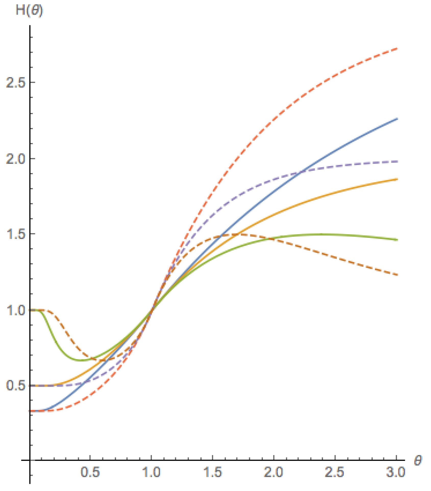
The correction function is given by
The structure of the H function was chosen so that when , then H is increasing and when , then H is non-monotonic. Thus, a fitted value of that is negative would indicate that the participant exhibits panicking behavior. Also, the parameter is such that .
Figure 4 shows members of this family of functions H.
The model function is given by
There are five parameters:
In order to be consistent with fitting the ESH2 model, the parameter was fixed to 1. We used a trust region type method to fit the four parameters. Unfortunately the objective function for the parameter fitting problem has multiple local minima. We started from 10 random starting points and picked the solution that gave the best objective value. (For session 3, participant 13, we started from 100 random starting points as the algorithm terminated with a local solution for only some of the starting points.)
Table 10 gives the leave-one-period-out LOOCV RMSE for each session.
The leave-one-session-out LOOCV RMSE is
It is also interesting to note that fitting a single set of parameters to all the participants in all the sessions gave an with the corresponding of . Thus, the behavior of the group can be described fairly well by a single set of parameters.
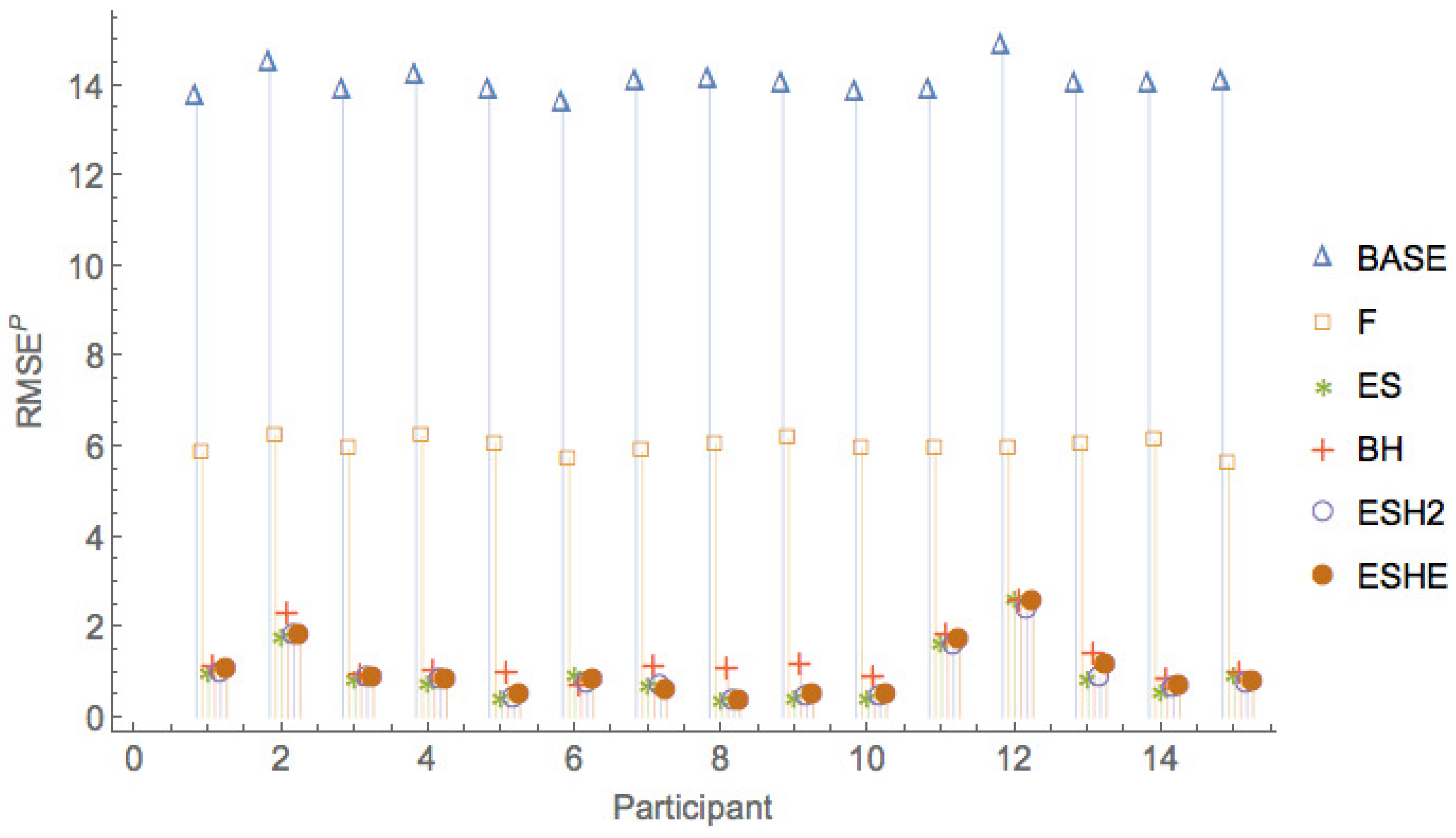
4.2.10. Comparison of Various Models
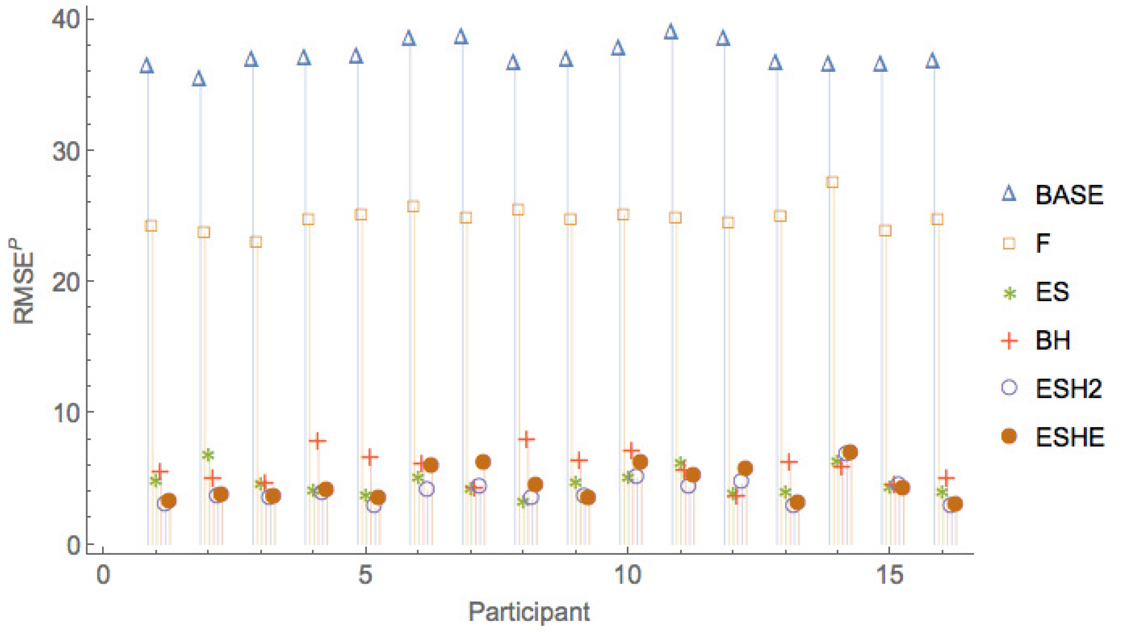
Figure 5, Figure 6 and Figure 7 show a comparison of the leave-one-period-out LOOCV RMSE of the various models. It can be seen that the pure rational expectations model (model ) has the highest errors throughout. When we allow the fundamental value to be fitted (model F), the errors are reduced, but the errors are still much larger than for the other models. The simple exponential smoothing model (model ) captures the participant forecasts remarkably well for a one-parameter model.
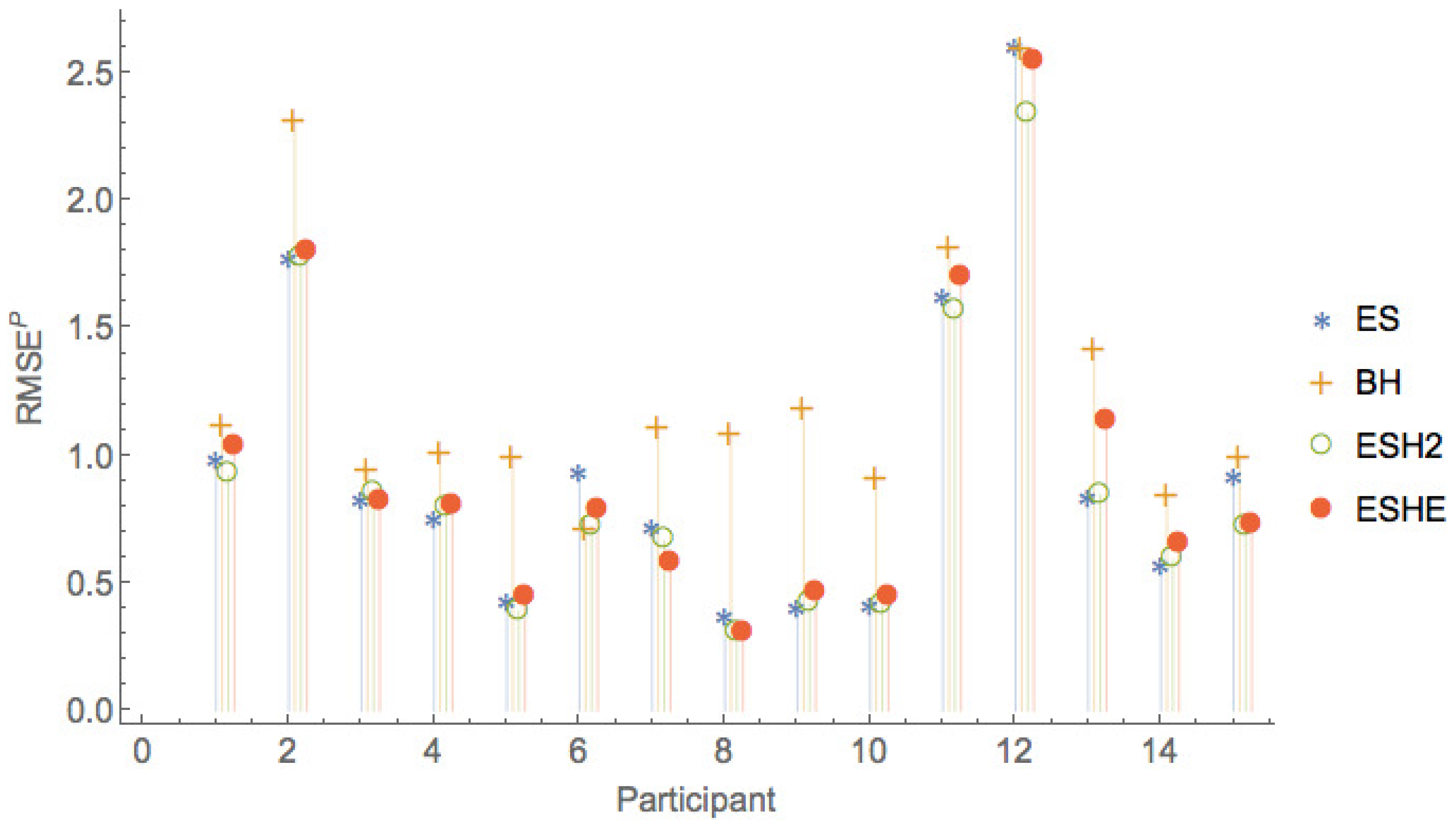
Figure 8, Figure 9 and Figure 10 show a comparison of the leave-one-period-out LOOCV RMSE of models , , , only, that is, leaving out the two worst performing models and F.
The leave-one-session-out LOOCV RMSE of the various models are given in Table 11. As is the case for the leave-one-period-out LOOCV RMSE, the rational expectations model () has the highest leave-one-session-out LOOCV RMSE, and model F has slightly smaller leave-one-session-out LOOCV RMSE. It can be seen that an exponential smoothing model with a single parameter for all sessions and all participants captures much of the variation in the observed forecasts. More sophisticated models with additional parameters ( and ) provide only small improvements in the leave-one-session-out LOOCV RMSE over what can be obtained with the model.
5. Interpretation and Implications of Results
In Cheriyan and Kleywegt (2016) the dynamical system associated with the price process was studied both analytically and numerically. It was shown there that the qualitative behavior of the trajectories of this dynamical system is determined by the parameter and the nature of the H function. These can also be related to the investors’ behavioral characteristics. Although the purpose of our experiment was to calibrate models of investor forecasting behavior and not to calibrate the dynamical system itself, in this section we make observations regarding the fitted models of investor forecasting behavior and the qualitative behavior of the dynamical system.
The parameter captures the investors’ memory—the weight that they put on the most recent observed price ratio. Given an H function and a fundamental dividend to price ratio (or price-earnings ratio ), a critical value of is given by
The slope of the H function at 1 captures investor confidence. If , it denotes cautious confidence, and if , it denotes excessive exuberance. It can be shown that if , then the fundamental value corresponds to a stable attracting point, that is, price trajectories that start in a neighborhood of the fundamental value, converge to the fundamental value. Numerical evidence suggests that the same is true for all trajectories, that is, if , then all price trajectories eventually converge to the fundamental value. If , then numerical results in Cheriyan and Kleywegt (2016) show that a price cycle appears that attracts all trajectories. This bifurcation process is continuous in the sense that the price cycles are small if is slightly larger than , and the price cycles gradually grow larger as increases from .
For not too far from , the price cycles appear to be predictable, that is, the price trajectories converge to a smooth curve, and any two trajectories that start close to each other will remain close to each other at all times. If the H function is monotonic, this behavior persists for . However, if H is non-monotonic, then for larger values of , the price trajectories can be non-predictable. This means that the trajectories do not converge to a smooth curve, and they exhibit sensitive dependence on initial conditions, that is, two trajectories that start close to each other will grow apart exponentially fast. A non-monotonic H captures what we called panicking behavior of the investor—as the extrapolation forecast increases beyond the fundamental value, the price forecast initially increases (confidence or exuberance), but beyond some value the price forecast decreases and moves closer to the fundamental value (panic).
Table 12 shows the fitted parameters for the model. For this function and . The fitted -values are all greater than the critical , and this is consistent with the price cycles observed in the three sessions.
Table 13 shows the fitted parameters for the model. It can be seen that the parameter is much larger than the critical . Once again, this is consistent with the observed price cycles. The slopes of the fitted H functions at the fundamental value, , are all close to 1. Some participants exhibit less exuberance (), and some exhibit more excessive exuberance (). All the fitted values for are positive—thus we do not find evidence of panicking behavior in the data.
Table 14 summarizes the fitted parameter values for the Brock and Homme model (). Brock and Hommes (1998) calls and the “bias” and “trend” parameters respectively. In particular, if , then the investor is called a “contrarian”, and if , then the investor is called a “trend chaser”. If and , then the investor is a “fundamentalist”. The fitted parameter values indicate that all the participants in our experiment were trend chasers.
6. Conclusions
We designed an experiment to study investors’ price forecast formation in the context of a market for an investment asset. Many experiments in the literature use trading runs with a pre-announced finite number of periods. However, the known end-of-horizon seems to affect participants’ forecasts, apparently via reasoning involving backward induction from the end of the horizon, that is not representative of forecasting in actual asset markets. In our experiment, we emulated an infinite horizon with discounting by stopping the trading run in each period with a pre-announced stopping probability. We conducted three experimental sessions with one trading run each. The equilibrium prices in all three trading runs exhibited cycles.
We fit a number of models of expectation formation to the data. The fit for the rational base case indicates that the rational expectations model does not provide an accurate model of investor forecasting behavior. Even when the fundamental value was replaced by a parameter that was fitted with the data (model F), the accuracy of the model did not improve much. (For example, the of the fit decreased from 22 to 18%). In contrast, a one-parameter exponential smoothing model gave remarkably accurate predictions of investor forecasts for such a simple model (with around ). Thus the evidence indicates that the investors, despite being reminded of the importance of the fundamental value of an investment asset and being told explicitly what the fundamental value was, resorted mostly to extrapolating from the past price data. Models with a larger number of parameters provided a slightly better fit. Moreover, it can be shown that these models are able to explain price cycles and more complex price trajectories in addition to price bubbles, see Cheriyan and Kleywegt (2016) for details. For every participant, the fitted value of was larger than the critical value for the associated dynamical system, which is consistent with the price cycles observed in the sessions. The parameter fits also indicated some amount of overconfidence. The data did not provide evidence of panicking behavior.
An interesting observation was the gap between theoretical knowledge and internalized knowledge. For example, based on correct answers to questions before the experiment, we concluded that the participants understood the meaning of the memoryless property of the geometric distribution and the computation of fundamental value. Nevertheless, their answers to questions and their trading behavior during the experiment seemed to indicate that they did not believe the theoretical properties. For example, the total number of periods in a trading run was a geometric random variable, and this was explained to the participants together with a reminder of the memoryless property of the geometric distribution. However, at the beginning of each period, each participant was asked to give the expected number of periods remaining in the trading run, and few participants gave the correct answer. It would be interesting to design an experiment that could lead to a better understanding of this apparent gap between theoretical and internalized knowledge.
Author Contributions
Vinod Cheriyan and Anton Kleywegt conceived the experiments; Federico Bonetto, Vinod Cheriyan and Anton Kleywegt designed and conducted the experiments; Vinod Cheriyan analyzed the data; Vinod Cheriyan and Anton Kleywegt wrote the paper; Federico Bonetto advised and provided revisions.
Conflicts of Interest
The authors declare no conflict of interest.
Appendix A. Fundamental Value Computations Corresponding to Different Dividend Processes
Appendix A.1. Deterministic Constant Dividend
Recall that in each period of the market, trades are made first and then the dividend is paid out. The dividend for each time period is a constant d. If the realization of a Geometric(p) random variable is a success, the salvage value s is paid out for each unit of stock held, otherwise, a new period starts. Algorithm A1 gives the details of the market algorithm for this case. Since the actual duration of the experiment is of the order of hours, we assume the discount factor is 0.
| Algorithm A1 Market Algorithm with Deterministic Constant Dividend |
|
Lemma 1.
In the setting of Market Algorithm A1, the fundamental value of a unit of stock is constant at each period and is given by
Proof.
Let be the random variable that is 1 if the market is running in period t and is 0 otherwise. Then is a sequence of iid Bernouilli() random variables. Let be the dividend in period t. We have that
Note that if any of the ’s are zero, then the entire expression is zero, this automatically captures the fact that if the market stops in period i, then for , . Also, for the present period, we know that the dividend is certain to be d, that is
The dividend stream at period t is given by
Now,
Therefore,
Now the dividend stream is
Now,
Therefore,
which is independent of t. Since a unit of stock held for ever necessarily will result in a final payout of s, and since the discount factor is 0, the fundamental value of a unit of stock is given by
☐
Remark.
Equation (A1) says that, in the case of deterministic dividends, probabilistic stopping of the market with stopping probability p is equivalent to an infinitely lived marked with discount factor .
Appendix A.2. Markov Dividends
In the case of Markov Dividends, the support of the dividend distribution in a period t depends on the market state in that period. The market states evolve according to a Markov chain with transition matrix P. Let denote the stationary distribution corresponding to transition matrix P. In our experiment, the initial state was drawn from the distribution .
Let the matrix Q denote the conditional p.m.f. for the dividend
and
Algorithm A2 gives the details of the market algorithm in the case of Markov dividends.
| Algorithm A2 Market Algorithm with Deterministic Constant Dividend |
Given:
Algorithm:
|
Participants have complete information about the parameters of the Markov Chain (Q, ) and but they do not know the underlying state process . They know that the market started in the steady state , that is is chosen according to .
They observe the prices and the dividends Let denote the history of dividends up to and including period .
Let . That is, is the estimate at the end of period t (i.e., beginning of period ) that the probability of the state will be . Let . In each period, the investor updates and uses it to compute the fundamental value for the next period.
The estimate of the probability distribution of the state is given by
Then, the fundamental value at period t can be computed as follows:
Now, for ,
Therefore
The next period’s fundamental value is given by
where
following similar calculations as above. Thus,
This was the fundamental value displayed to the participants.
Next,
and
Thus, at the beginning of period t, the investor forms the expectation as follows:
Appendix B. Details of Leave-One-Out-Cross-Validation Approach
To compare different models that were fitted, we used Leave-One-Out-Cross-Validation (LOOCV) approach. We perform LOOCV with two types of subsets (1) leave-one-period-out LOOCV and (2) leave-one-session-out LOOCV
For reference, the notation we use is repeated below:
(, as discussed in the main body.)
Consider a family of models of forecast formation represented as
where denotes the vector of parameters of the model and are i.i.d. random variables.
The parameter fit for participant u in session is given by
The parameter fit using all data in all sessions is given by
Leave-One-Period-Out LOOCV
In this case, separate parameters are fit for each individual participant. The resulting RMSE gives a measure of predictability when a separate model is fitted for each participant. The leave-one-period-out LOOCV RMSE for a participant is computed as follows.
Let denote the vector of parameters fitted for the participant u in session after dropping the data for period i. That is,
Then, the leave-one-period-out LOOCV RMSE of the model for the participant is given by
The leave-one-period-out LOOCV coefficient of variation is the leave-one-period-out LOOCV RMSE scaled by the fundamental value, given by
Leave-One-Session-Out LOOCV
In this case, one set of parameters are fit for all participants and all periods in all sessions but one (thus in two sessions). The fitted model is then used to calculate forecasts for all particpants and all periods in the omitted session. The resulting RMSE gives a measure of predictability if a common model is fitted for all sessions and participants.
The leave-one-session-out LOOCV RMSE is computed as follows. Let denote the vector of parameters fitted after dropping all observations in session s. That is,
Then, the leave-one-session-out LOOCV RMSE is given by
The leave-one-session-out LOOCV coefficient of variation is the leave-one-session-out LOOCV RMSE scaled by the fundamental value, given by
References
- Armstrong, Scott J. 1985. Long-Range Forecasting: From Crystal Ball to Computer, 2nd ed. New York: John Wiley & Sons. [Google Scholar]
- Ball, Sheryl B., and Charles A. Holt. 1998. Classroom games: Speculation and bubbles in an asset market. The Journal of Economic Perspectives 12: 207–18. [Google Scholar] [CrossRef]
- Brock, William A., and Cars H. Hommes. 1997. A rational route to randomness. Econometrica 65: 1059–95. [Google Scholar] [CrossRef]
- Brock, William A., and Cars H. Hommes. 1998. Heterogeneous beliefs and routes to chaos in a simple asset pricing model. Journal of Economic Dynamics and Control 22: 1235–74. [Google Scholar] [CrossRef]
- Camerer, Colin F., and Keith Weigelt. 1993. Convergence in experimental double auctions in stochastically lived assets. In The Double Auction Market: Institutions, Theories and Evidence. Reading: Addison–Wesley, pp. 355–59. [Google Scholar]
- Campbell, John Y., and Robert J. Shiller. 1987. Cointegration and tests of present value models. The Journal of Political Economy 95: 1062–88. [Google Scholar] [CrossRef]
- Campbell, John Y., and Robert J. Shiller. 1988. The dividend-price ratio and expectations of future dividends and discount factors. The Review of Financial Studies 1: 195–228. [Google Scholar] [CrossRef]
- Cheriyan, Vinod, and Anton J. Kleywegt. 2016. A dynamical systems model of price bubbles and cycles. Quantitative Finance 16: 309–36. [Google Scholar] [CrossRef]
- Chuang, Wen I., and Bong-Soo Lee. 2006. An empirical evaluation of the overconfidence hypothesis. Journal of Banking & Finance 30: 2489–515. [Google Scholar]
- Hirota, Shinichi, and Shyam Sunder. 2007. Price bubbles sans dividend anchors: Evidence from laboratory stock markets. Journal of Economic Dynamics and Control 31: 1875–909. [Google Scholar] [CrossRef]
- LeRoy, Stephen F., and Richard D. Porter. 1981. The present-value relation: Tests based on implied variance bounds. Econometrica 49: 555–74. [Google Scholar] [CrossRef]
- LeRoy, Stephen F. 1989. Efficient capital markets and martingales. Journal of Economic Literature 27: 1583–621. [Google Scholar]
- Lugovskyy, Volodymyr, Daniela Puzzello, and Steven Tucker. 2009. An Experimental Study of Bubble Formation in Asset Markets Using the Tâtonnement Pricing Mechanism. Working Paper. Christchurch: University of Canterbury. [Google Scholar]
- Nickerson, Mike, Yaron Lahav, and Charles N. Noussair. 2007. Traders’ expectations in asset markets: Experimental evidence. The American Economic Review 97: 1901–20. [Google Scholar]
- Ramnath, Sundaresh, Steve Rock, and Philip Shane. 2008. The financial analyst forecasting literature: A taxonomy with suggestions for further research. International Journal of Forecasting 24: 34–75. [Google Scholar] [CrossRef]
- Scheinkman, Jose A., and Wei Xiong. 2003. Overconfidence and speculative bubbles. Journal of Political Economy 111: 1183–219. [Google Scholar] [CrossRef]
- Shiller, Robert J. 1981a. Do stock prices move too much to be justified by subsequent changes in dividends? The American Economic Review 71: 421–36. [Google Scholar]
- Shiller, Robert J. 1981b. The use of volatility measures in assessing market efficiency. The Journal of Finance 36: 291–304. [Google Scholar]
- Shiller, Robert J. 1986. The Marsh-Merton model of managers’ smoothing of dividends. The American Economic Review 76: 499–503. [Google Scholar]
- Smith, Vernon L., Gerry L. Suchanek, and Arlington W. Williams. 1988. Bubbles, crashes, and endogenous expectations in experimental spot asset markets. Econometrica: Journal of the Econometric Society 56: 1119–51. [Google Scholar] [CrossRef]
- Tversky, Amos, and Daniel Kahneman. 1974. Judgment under uncertainty: Heuristics and biases. Science 185: 1124–31. [Google Scholar] [CrossRef] [PubMed]
- West, Kenneth D. 1988a. Dividend innovations and stock price volatility. Econometrica 56: 37–61. [Google Scholar] [CrossRef]
- West, Kenneth D. 1988b. Bubbles, fads and stock price volatility tests: A partial evaluation. The Journal of Finance 43: 639–56. [Google Scholar] [CrossRef]
- Wong, Wing-Keung, and Raymond Chan. 2004. On the estimation of cost of capital and its reliability. Quantitative Finance 4: 365–72. [Google Scholar] [CrossRef]
Figure 1.
Equilibrium Prices from Sessions 1–3 (Sub-figures (a)–(c) respectively).

Figure 2.
Price forecasts for each period from Sessions 1–3 (Sub-figures (a)–(c) respectively).
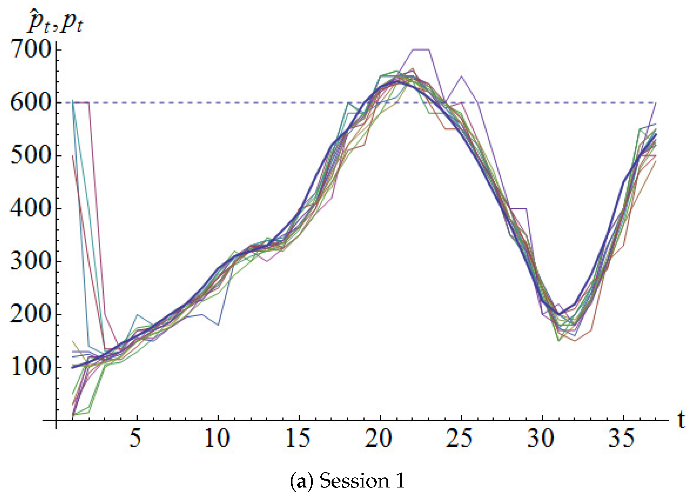

Figure 3.
Data fit for Participant 14 in Session 1. Note that the first 10 periods were used for priming, hence are not included in the data fit.
Figure 3.
Data fit for Participant 14 in Session 1. Note that the first 10 periods were used for priming, hence are not included in the data fit.
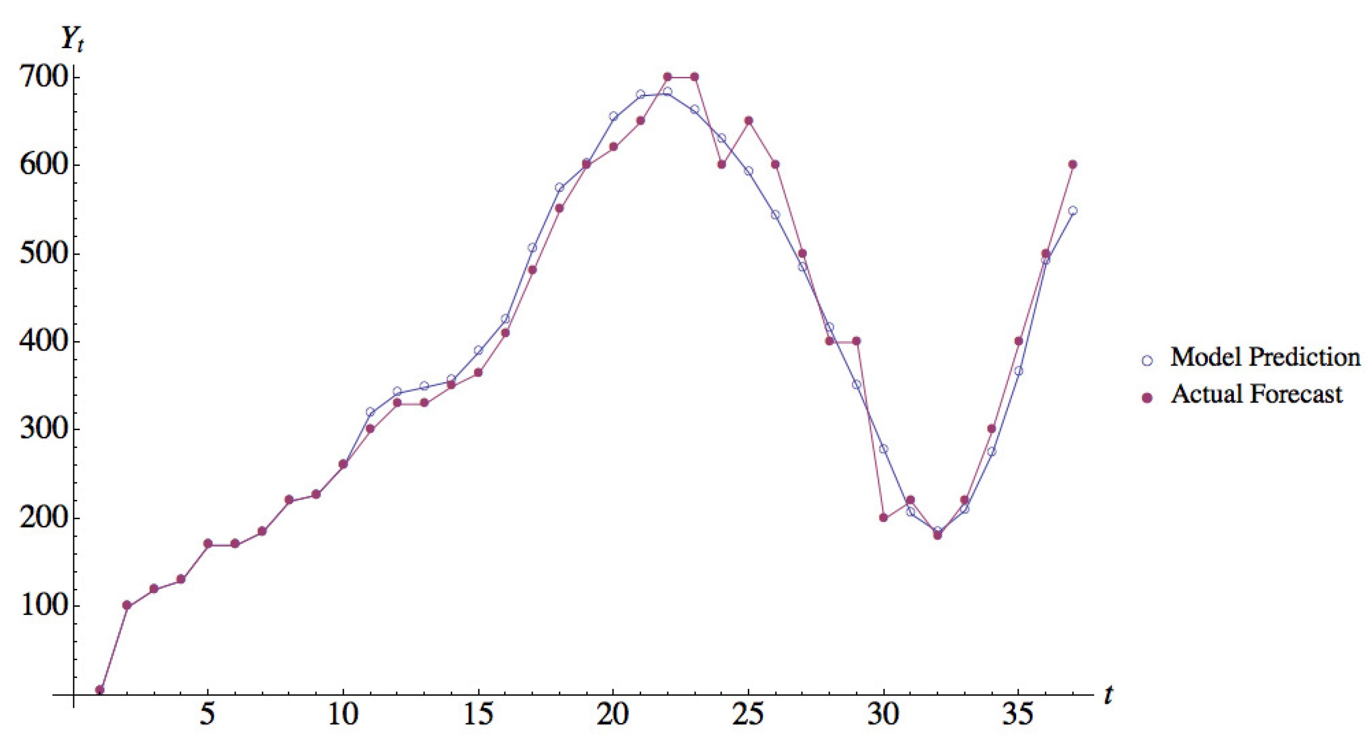
Figure 4.
Members from the family of functions. The solid lines are for () and the dotted lines are for (). For each , functions are plotted for . When , the function is non-monotonic, as defined in the main text.
Figure 4.
Members from the family of functions. The solid lines are for () and the dotted lines are for (). For each , functions are plotted for . When , the function is non-monotonic, as defined in the main text.

Figure 5.
Comparison of leave-one-period-out LOOCV RMSE of all models for Session 1.

Figure 6.
Comparison of leave-one-period-out LOOCV RMSE of all models for Session 2.
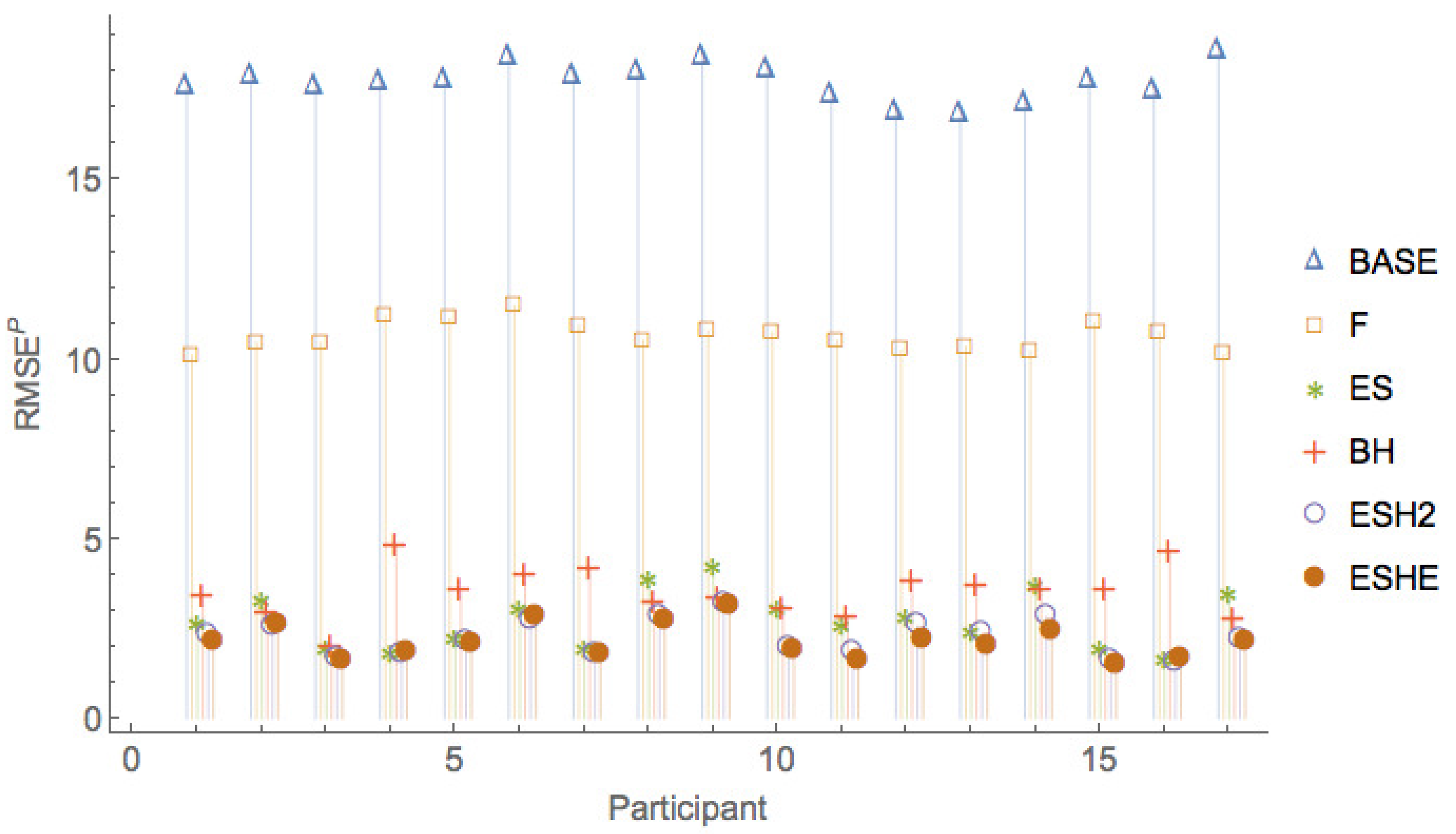
Figure 7.
Comparison of leave-one-period-out LOOCV RMSE of all models for Session 3.

Figure 8.
Comparison of leave-one-period-out LOOCV RMSE of selected models for Session 1.
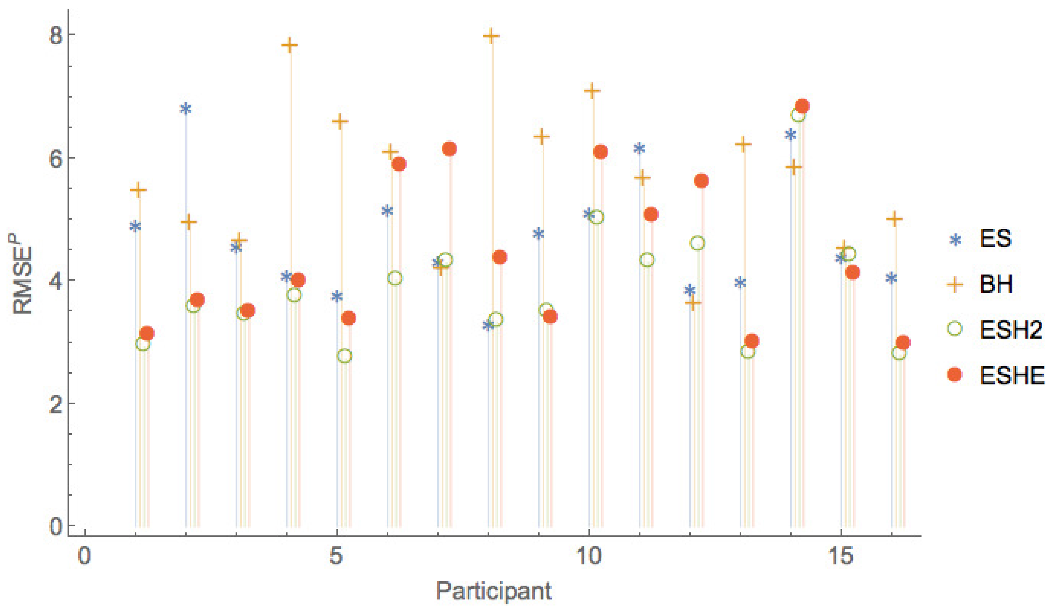
Figure 9.
Comparison of leave-one-period-out LOOCV RMSE of selected models for Session 2.

Figure 10.
Comparison of leave-one-period-out LOOCV RMSE of selected models for Session 3.


Table 1.
Conditional probability mass function for the dividends.
| Market State | ||||
|---|---|---|---|---|
| low | ||||
| high |
Table 2.
Parameters for the Experimental Sessions.
| Session | Participants | Periods | Dividend Type | Mean Dividend (ECUs) | Salvage Value (ECUs) |
|---|---|---|---|---|---|
| 1 | 16 | 37 | Constant | 10 | 100 |
| 2 | 17 | 64 | Constant | 10 | 100 |
| 3 | 15 | 72 | Markovian | 10 | 100 |
Table 3.
Expected earnings for the three sessions.
| Session | Participants | Number of Valid Responses | Average Expected Win | Average of Prize Money Per Participant |
|---|---|---|---|---|
| 1 | 16 | 14 | 90.43 | 31.25 |
| 2 | 17 | 15 | 66.07 | 29.41 |
| 3 | 15 | 13 | 68.91 | 33.33 |
Table 4.
Details of the models fit to the data.
| Model () | Generalized Mean (m) | Correction Function (H) | Parameters to Fit |
|---|---|---|---|
| N/A | N/A | None | |
| F | N/A | N/A | |
| Exponential Smoothing | |||
| N/A | N/A | ||
| Exponential Smoothing | |||
| Exponential Smoothing |
Table 5.
Forecast errors of the rational base case for the three sessions.
| Session 1 | Session 2 | Session 3 | ||||
|---|---|---|---|---|---|---|
| Part. | ||||||
| 1 | 217.66 | 36.2767 | 105.273 | 17.5455 | 82.291 | 13.7152 |
| 2 | 211.608 | 35.2679 | 107.251 | 17.8752 | 86.6954 | 14.4492 |
| 3 | 220.79 | 36.7983 | 105.178 | 17.5297 | 83.2023 | 13.8671 |
| 4 | 221.015 | 36.8358 | 106.147 | 17.6911 | 84.9293 | 14.1549 |
| 5 | 221.923 | 36.9872 | 106.301 | 17.7169 | 82.9877 | 13.8313 |
| 6 | 230.33 | 38.3883 | 110.223 | 18.3705 | 81.2825 | 13.5471 |
| 7 | 231.04 | 38.5067 | 107.187 | 17.8645 | 84.3218 | 14.0536 |
| 8 | 218.861 | 36.4768 | 107.866 | 17.9777 | 84.3693 | 14.0615 |
| 9 | 220.128 | 36.6881 | 110.193 | 18.3655 | 84.007 | 14.0012 |
| 10 | 225.415 | 37.5692 | 108.192 | 18.0321 | 82.7644 | 13.7941 |
| 11 | 233.164 | 38.8607 | 103.875 | 17.3125 | 82.9435 | 13.8239 |
| 12 | 230.39 | 38.3984 | 101.052 | 16.8421 | 88.9848 | 14.8308 |
| 13 | 218.782 | 36.4637 | 100.625 | 16.7709 | 84.0285 | 14.0048 |
| 14 | 218.338 | 36.3896 | 102.668 | 17.1114 | 83.792 | 13.9653 |
| 15 | 218.261 | 36.3769 | 106.432 | 17.7386 | 84.16 | 14.0267 |
| 16 | 219.511 | 36.5852 | 104.591 | 17.4318 | – | – |
| 17 | – | – | 111.329 | 18.5549 | – | – |
Table 6.
Forecast errors of the modified rational expectations model for the three sessions.
| Session 1 | Session 2 | Session 3 | ||||
|---|---|---|---|---|---|---|
| Part. | ||||||
| 1 | 145.378 | 24.2296 | 60.6133 | 10.1022 | 35.165 | 5.86083 |
| 2 | 142.013 | 23.6689 | 62.7894 | 10.4649 | 37.508 | 6.25133 |
| 3 | 138.032 | 23.0054 | 62.7262 | 10.4544 | 35.6265 | 5.93775 |
| 4 | 147.772 | 24.6287 | 67.3448 | 11.2241 | 37.2925 | 6.21542 |
| 5 | 150.402 | 25.067 | 66.8102 | 11.135 | 36.3315 | 6.05525 |
| 6 | 153.929 | 25.6548 | 68.9046 | 11.4841 | 34.4464 | 5.74107 |
| 7 | 148.482 | 24.747 | 65.6383 | 10.9397 | 35.3149 | 5.88582 |
| 8 | 152.481 | 25.4135 | 63.1547 | 10.5258 | 36.3194 | 6.05323 |
| 9 | 147.757 | 24.6262 | 64.7539 | 10.7923 | 37.0776 | 6.1796 |
| 10 | 150.344 | 25.0573 | 64.4885 | 10.7481 | 35.7969 | 5.96614 |
| 11 | 149.164 | 24.8606 | 63.1322 | 10.522 | 35.7003 | 5.95006 |
| 12 | 146.896 | 24.4826 | 61.5347 | 10.2558 | 35.776 | 5.96267 |
| 13 | 149.369 | 24.8949 | 62.0644 | 10.3441 | 36.2216 | 6.03693 |
| 14 | 164.938 | 27.4897 | 61.362 | 10.227 | 36.8212 | 6.13687 |
| 15 | 143.054 | 23.8424 | 66.0542 | 11.009 | 33.6933 | 5.61555 |
| 16 | 148.349 | 24.7248 | 64.5339 | 10.7556 | – | – |
| 17 | – | – | 60.7467 | 10.1245 | – | – |
Table 7.
Forecast errors of the simple exponential smoothing model (ES) for the three sessions.
| Session 1 | Session 2 | Session 3 | ||||
|---|---|---|---|---|---|---|
| Part. | ||||||
| 1 | 29.3523 | 4.89205 | 15.9516 | 2.65859 | 5.87511 | 0.979186 |
| 2 | 40.8778 | 6.81297 | 19.5621 | 3.26035 | 10.589 | 1.76483 |
| 3 | 27.4048 | 4.56746 | 11.6133 | 1.93555 | 4.95529 | 0.825882 |
| 4 | 24.4905 | 4.08174 | 10.7994 | 1.7999 | 4.47145 | 0.745242 |
| 5 | 22.6001 | 3.76669 | 13.1662 | 2.19436 | 2.5535 | 0.425584 |
| 6 | 30.8664 | 5.14439 | 18.1567 | 3.02612 | 5.59091 | 0.931818 |
| 7 | 25.7927 | 4.29878 | 11.5305 | 1.92175 | 4.30922 | 0.718204 |
| 8 | 19.7088 | 3.2848 | 23.1764 | 3.86274 | 2.18925 | 0.364875 |
| 9 | 28.7235 | 4.78725 | 25.3742 | 4.22903 | 2.41359 | 0.402265 |
| 10 | 30.5402 | 5.09003 | 18.3046 | 3.05077 | 2.45213 | 0.408688 |
| 11 | 37.0004 | 6.16673 | 15.4212 | 2.57019 | 9.71214 | 1.61869 |
| 12 | 23.1125 | 3.85208 | 16.7412 | 2.7902 | 15.5948 | 2.59914 |
| 13 | 23.9457 | 3.99094 | 14.3645 | 2.39408 | 5.01824 | 0.836374 |
| 14 | 38.4261 | 6.40435 | 22.18 | 3.69666 | 3.39276 | 0.56546 |
| 15 | 26.3165 | 4.38609 | 11.7149 | 1.95248 | 5.50357 | 0.917261 |
| 16 | 24.3416 | 4.05693 | 9.91197 | 1.65199 | – | – |
| 17 | – | – | 20.8576 | 3.47626 | – | – |
Table 8.
Forecast errors of the Brock and Homme model (BH) for the three sessions.
| Session 1 | Session 2 | Session 3 | ||||
|---|---|---|---|---|---|---|
| Part. | ||||||
| 1 | 32.8829 | 5.48048 | 20.4555 | 3.40925 | 6.66709 | 1.11118 |
| 2 | 29.7489 | 4.95815 | 17.6728 | 2.94547 | 13.8489 | 2.30816 |
| 3 | 27.9104 | 4.65174 | 12.0573 | 2.00956 | 5.62034 | 0.936723 |
| 4 | 47.0301 | 7.83836 | 28.9688 | 4.82813 | 6.04289 | 1.00715 |
| 5 | 39.5275 | 6.58791 | 21.3855 | 3.56425 | 5.9418 | 0.990301 |
| 6 | 36.5602 | 6.09336 | 23.8271 | 3.97118 | 4.24954 | 0.708256 |
| 7 | 25.3059 | 4.21766 | 25.054 | 4.17567 | 6.6485 | 1.10808 |
| 8 | 47.8765 | 7.97942 | 19.1891 | 3.19819 | 6.48157 | 1.08026 |
| 9 | 38.0958 | 6.3493 | 20.0471 | 3.34118 | 7.09285 | 1.18214 |
| 10 | 42.571 | 7.09516 | 18.366 | 3.061 | 5.41897 | 0.903162 |
| 11 | 33.9904 | 5.66506 | 16.9797 | 2.82995 | 10.8703 | 1.81171 |
| 12 | 21.7463 | 3.62438 | 22.785 | 3.7975 | 15.5483 | 2.59138 |
| 13 | 37.3059 | 6.21766 | 22.0264 | 3.67107 | 8.46553 | 1.41092 |
| 14 | 35.1063 | 5.85105 | 21.3216 | 3.5536 | 5.02028 | 0.836713 |
| 15 | 27.1887 | 4.53146 | 21.4652 | 3.57754 | 5.9336 | 0.988934 |
| 16 | 30.092 | 5.01533 | 27.8947 | 4.64912 | – | – |
| 17 | – | – | 16.5292 | 2.75487 | – | – |
Table 9.
Forecast errors of the exponential smoothing with quadratic H model (ESH2) for the three sessions.
Table 9.
Forecast errors of the exponential smoothing with quadratic H model (ESH2) for the three sessions.
| Session 1 | Session 2 | Session 3 | ||||
|---|---|---|---|---|---|---|
| Part. | ||||||
| 1 | 17.6051 | 2.93419 | 13.802 | 2.30033 | 5.51619 | 0.919365 |
| 2 | 21.4067 | 3.56779 | 15.2125 | 2.53541 | 10.6341 | 1.77234 |
| 3 | 20.5887 | 3.43145 | 9.95013 | 1.65835 | 5.08502 | 0.847504 |
| 4 | 22.3997 | 3.73329 | 10.5322 | 1.75536 | 4.72411 | 0.787352 |
| 5 | 16.3869 | 2.73115 | 12.4787 | 2.07978 | 2.33086 | 0.388477 |
| 6 | 24.1159 | 4.01932 | 16.2193 | 2.70322 | 4.31467 | 0.719111 |
| 7 | 25.7992 | 4.29986 | 10.4045 | 1.73408 | 3.99644 | 0.666073 |
| 8 | 20.0133 | 3.33556 | 16.7847 | 2.79745 | 1.7952 | 0.2992 |
| 9 | 20.9099 | 3.48498 | 19.0443 | 3.17404 | 2.51195 | 0.418658 |
| 10 | 29.9577 | 4.99294 | 11.6179 | 1.93631 | 2.45609 | 0.409348 |
| 11 | 25.8743 | 4.31238 | 10.7424 | 1.79041 | 9.38085 | 1.56348 |
| 12 | 27.5461 | 4.59102 | 15.3596 | 2.55993 | 14.0158 | 2.33596 |
| 13 | 16.84 | 2.80667 | 13.9764 | 2.3294 | 5.06343 | 0.843905 |
| 14 | 39.9483 | 6.65804 | 16.9594 | 2.82657 | 3.5487 | 0.59145 |
| 15 | 26.4518 | 4.40863 | 9.33683 | 1.55614 | 4.29295 | 0.715491 |
| 16 | 16.7662 | 2.79437 | 9.04149 | 1.50691 | – | – |
| 17 | – | – | 12.9543 | 2.15905 | – | – |
Table 10.
Forecast errors of the exponential smoothing with non-monotonic H model (ESHE) for the three sessions.
Table 10.
Forecast errors of the exponential smoothing with non-monotonic H model (ESHE) for the three sessions.
| Session 1 | Session 2 | Session 3 | ||||
|---|---|---|---|---|---|---|
| Part. | ||||||
| 1 | 18.6982 | 3.11636 | 12.5044 | 2.08407 | 6.17827 | 1.02971 |
| 2 | 21.986 | 3.66434 | 15.4513 | 2.57522 | 10.7462 | 1.79103 |
| 3 | 20.8771 | 3.47952 | 9.51516 | 1.58586 | 4.90735 | 0.817892 |
| 4 | 23.9088 | 3.9848 | 10.8678 | 1.81129 | 4.80413 | 0.800689 |
| 5 | 20.2253 | 3.37088 | 12.3063 | 2.05104 | 2.64659 | 0.441099 |
| 6 | 35.2502 | 5.87503 | 16.6865 | 2.78108 | 4.70287 | 0.783811 |
| 7 | 36.7429 | 6.12382 | 10.6514 | 1.77524 | 3.46634 | 0.577723 |
| 8 | 26.1145 | 4.35242 | 16.0153 | 2.66922 | 1.82649 | 0.304415 |
| 9 | 20.3506 | 3.39177 | 18.5346 | 3.08909 | 2.73675 | 0.456125 |
| 10 | 36.3602 | 6.06004 | 11.1061 | 1.85102 | 2.66171 | 0.443618 |
| 11 | 30.3859 | 5.06431 | 9.52843 | 1.58807 | 10.1615 | 1.69359 |
| 12 | 33.5378 | 5.58963 | 12.8078 | 2.13464 | 15.2613 | 2.54355 |
| 13 | 17.9947 | 2.99912 | 12.0823 | 2.01372 | 6.77343 | 1.12891 |
| 14 | 40.8638 | 6.81063 | 14.4793 | 2.41322 | 3.90796 | 0.651326 |
| 15 | 24.6398 | 4.10663 | 8.80488 | 1.46748 | 4.32493 | 0.720822 |
| 16 | 17.7253 | 2.95421 | 9.94192 | 1.65699 | – | – |
| 17 | – | – | 12.5098 | 2.08496 | – | – |
Table 11.
Comparison of leave-one-session-out LOOCV RMSE of various models.
| Model | No. of Parameters | ||
|---|---|---|---|
| BASE | 0 | 150.34 | 25.06 |
| F | 1 | 109.04 | 18.17 |
| ES | 1 | 22.87 | 3.81 |
| BH | 2 | 23.97 | 3.99 |
| ESH2 | 3 | 19.51 | 3.25 |
| ESHE | 4 | 19.25 | 3.21 |
Table 12.
Fitted parameters for quadratic H model () for the three sessions.
| Session 1 | Session 2 | Session 3 | ||||||||||
|---|---|---|---|---|---|---|---|---|---|---|---|---|
| Part. | CV (%) | CV (%) | CV (%) | |||||||||
| 1 | 0.35 | 0.01 | 172.32 | 2.6 | 0.73 | 0.18 | 365.69 | 1.94 | 0.6 | 2.26 | 543.41 | 0.78 |
| 2 | 0.24 | 0.52 | 407.91 | 3.03 | 0.43 | 0.36 | 395.39 | 2.34 | 0.49 | 0.03 | 312.63 | 1.7 |
| 3 | 0.29 | 0.01 | 141.31 | 3.12 | 0.15 | 0.07 | 317.4 | 1.54 | 0.56 | 1.69 | 493.54 | 0.76 |
| 4 | 0.99 | 0.01 | 186.84 | 3.52 | 0.99 | 0.11 | 413.81 | 1.71 | 0.99 | 0.61 | 488.64 | 0.72 |
| 5 | 0.49 | 0.01 | 179.32 | 2.51 | 0.62 | 0.19 | 405.06 | 1.9 | 0.72 | 0.08 | 697.33 | 0.37 |
| 6 | 0.39 | 0.01 | 167.4 | 3.86 | 0.5 | 0.01 | 214.67 | 2.48 | 0.09 | 1.69 | 452.22 | 0.6 |
| 7 | 0.17 | 0.01 | 146.57 | 3.87 | 0.99 | 0.03 | 298.27 | 1.64 | 0.84 | 1.37 | 475.69 | 0.58 |
| 8 | 0.99 | 0.01 | 250.59 | 3.23 | 0.44 | 0.23 | 370.67 | 2.52 | 0.49 | 0.89 | 472.42 | 0.25 |
| 9 | 0.38 | 0.28 | 371.52 | 2.89 | 0.49 | 0.1 | 321.78 | 2.83 | 0.94 | 0.01 | 816.76 | 0.37 |
| 10 | 0.47 | 0.01 | 168.01 | 4.01 | 0.35 | 0.06 | 302.52 | 1.78 | 0.71 | 0.19 | 643.85 | 0.31 |
| 11 | 0.25 | 0.01 | 142.26 | 3.96 | 0.42 | 0.36 | 414.8 | 1.62 | 0.51 | 1.18 | 569.84 | 1.53 |
| 12 | 0.19 | 0.01 | 143.75 | 4 | 0.99 | 1.06 | 473.49 | 2.24 | 0.99 | 3.17 | 460.64 | 2.21 |
| 13 | 0.35 | 0.01 | 184.62 | 2.58 | 0.96 | 1.08 | 490.54 | 2.04 | 0.99 | 1.95 | 498.14 | 0.78 |
| 14 | 0.19 | 0.08 | 448.71 | 5.43 | 0.51 | 0.79 | 444.85 | 2.43 | 0.47 | 0.06 | 419.71 | 0.53 |
| 15 | 0.23 | 0.42 | 394.28 | 3.55 | 0.57 | 0.12 | 370.91 | 1.37 | 0.52 | 3.45 | 482.54 | 0.6 |
| 16 | 0.35 | 0.01 | 175.67 | 2.67 | 0.99 | 0.05 | 351.82 | 1.47 | – | – | – | – |
| 17 | – | – | – | – | 0.34 | 0.09 | 291.93 | 1.99 | – | – | – | – |
Table 13.
Fitted parameters for exponential smoothing with non-monotonic H model (ESHE) for the three sessions.
Table 13.
Fitted parameters for exponential smoothing with non-monotonic H model (ESHE) for the three sessions.
| Session 1 | Session 2 | Session 3 | ||||||||||
|---|---|---|---|---|---|---|---|---|---|---|---|---|
| Part. | ||||||||||||
| 1 | 0.349 | −0.003 | 0.874 | 1.019 | 0.604 | −0.101 | 0.800 | 1.131 | 0.012 | −0.122 | 1.000 | 1.158 |
| 2 | 0.246 | −0.051 | 0.365 | 1.071 | 0.433 | −0.086 | 1.000 | 1.113 | 0.445 | 0.002 | 0.916 | 1.014 |
| 3 | 0.300 | 0.031 | 0.871 | 0.986 | 0.172 | 0.102 | 0.928 | 0.922 | 0.550 | −0.069 | 0.905 | 1.092 |
| 4 | 0.990 | −0.060 | 0.862 | 1.082 | 0.990 | −0.036 | 0.915 | 1.055 | 0.990 | −0.023 | 0.393 | 1.041 |
| 5 | 0.470 | −0.052 | 0.872 | 1.072 | 0.595 | −0.046 | 0.876 | 1.065 | 0.610 | −0.028 | 0.253 | 1.046 |
| 6 | 0.463 | −0.369 | 0.810 | 1.610 | 0.550 | −0.163 | 0.847 | 1.215 | 0.336 | −0.117 | 0.807 | 1.152 |
| 7 | 0.182 | −0.008 | 0.872 | 1.024 | 0.990 | 0.002 | 0.917 | 1.015 | 0.874 | −0.074 | 0.362 | 1.098 |
| 8 | 0.990 | −0.087 | 0.866 | 1.114 | 0.439 | −0.070 | 0.568 | 1.094 | 0.478 | −0.013 | 0.484 | 1.030 |
| 9 | 0.384 | −0.048 | 0.945 | 1.068 | 0.475 | −0.034 | 0.731 | 1.053 | 0.901 | −0.022 | 0.961 | 1.040 |
| 10 | 0.457 | −0.035 | 0.873 | 1.054 | 0.355 | 0.080 | 0.908 | 0.942 | 0.667 | 0.020 | 0.946 | 0.997 |
| 11 | 0.248 | −0.042 | 0.858 | 1.061 | 0.423 | −0.110 | 0.811 | 1.142 | 0.393 | −0.065 | 0.570 | 1.088 |
| 12 | 0.205 | 0.003 | 0.873 | 1.013 | 0.990 | −0.159 | 0.116 | 1.209 | 0.990 | −0.131 | 0.846 | 1.170 |
| 13 | 0.342 | −0.048 | 0.868 | 1.067 | 0.686 | −0.146 | 0.805 | 1.190 | 0.010 | −0.135 | 0.937 | 1.176 |
| 14 | 0.194 | −0.161 | 1.000 | 1.212 | 0.479 | −0.148 | 1.000 | 1.194 | 0.422 | −0.012 | 0.948 | 1.029 |
| 15 | 0.230 | 0.016 | 0.886 | 1.001 | 0.547 | −0.040 | 0.849 | 1.059 | 0.568 | −0.113 | 0.255 | 1.146 |
| 16 | 0.347 | −0.037 | 0.870 | 1.056 | 0.990 | 0.040 | 0.938 | 0.977 | – | – | – | – |
| 17 | – | – | – | – | 0.343 | −0.022 | 0.746 | 1.039 | – | – | – | – |
Table 14.
Summary of fitted slope parameters for model .
| Session | ||||||
|---|---|---|---|---|---|---|
| 1 | −12.87 | 4.78 | 45.11 | 0.95 | 1.02 | 1.14 |
| 2 | −12.74 | −1.69 | 4.35 | 0.93 | 0.98 | 1.05 |
| 3 | −6.63 | 4.61 | 8.59 | 1.01 | 1.09 | 1.15 |
© 2017 by the authors. Licensee MDPI, Basel, Switzerland. This article is an open access article distributed under the terms and conditions of the Creative Commons Attribution (CC BY) license (http://creativecommons.org/licenses/by/4.0/).
Share and Cite
MDPI and ACS Style
Bonetto, F.; Cheriyan, V.; Kleywegt, A.J. Models of Investor Forecasting Behavior — Experimental Evidence. J. Risk Financial Manag. 2018, 11, 3. https://doi.org/10.3390/jrfm11010003
AMA Style
Bonetto F, Cheriyan V, Kleywegt AJ. Models of Investor Forecasting Behavior — Experimental Evidence. Journal of Risk and Financial Management. 2018; 11(1):3. https://doi.org/10.3390/jrfm11010003
Chicago/Turabian StyleBonetto, Federico, Vinod Cheriyan, and Anton J. Kleywegt. 2018. "Models of Investor Forecasting Behavior — Experimental Evidence" Journal of Risk and Financial Management 11, no. 1: 3. https://doi.org/10.3390/jrfm11010003