Best Fitting Fat Tail Distribution for the Volatilities of Energy Futures: Gev, Gat and Stable Distributions in GARCH and APARCH Models


Abstract
:1. Introduction
2. Literature Review
3. Methodology
3.1. GARCH and APARCH Model
3.2. Alpha-Stable Distribution
3.3. Generalized Extreme Values (GEV) Distribution
3.4. Gat Distribution
4. Empirical Analysis
4.1. Unit Root Test
4.2. Normality Tests
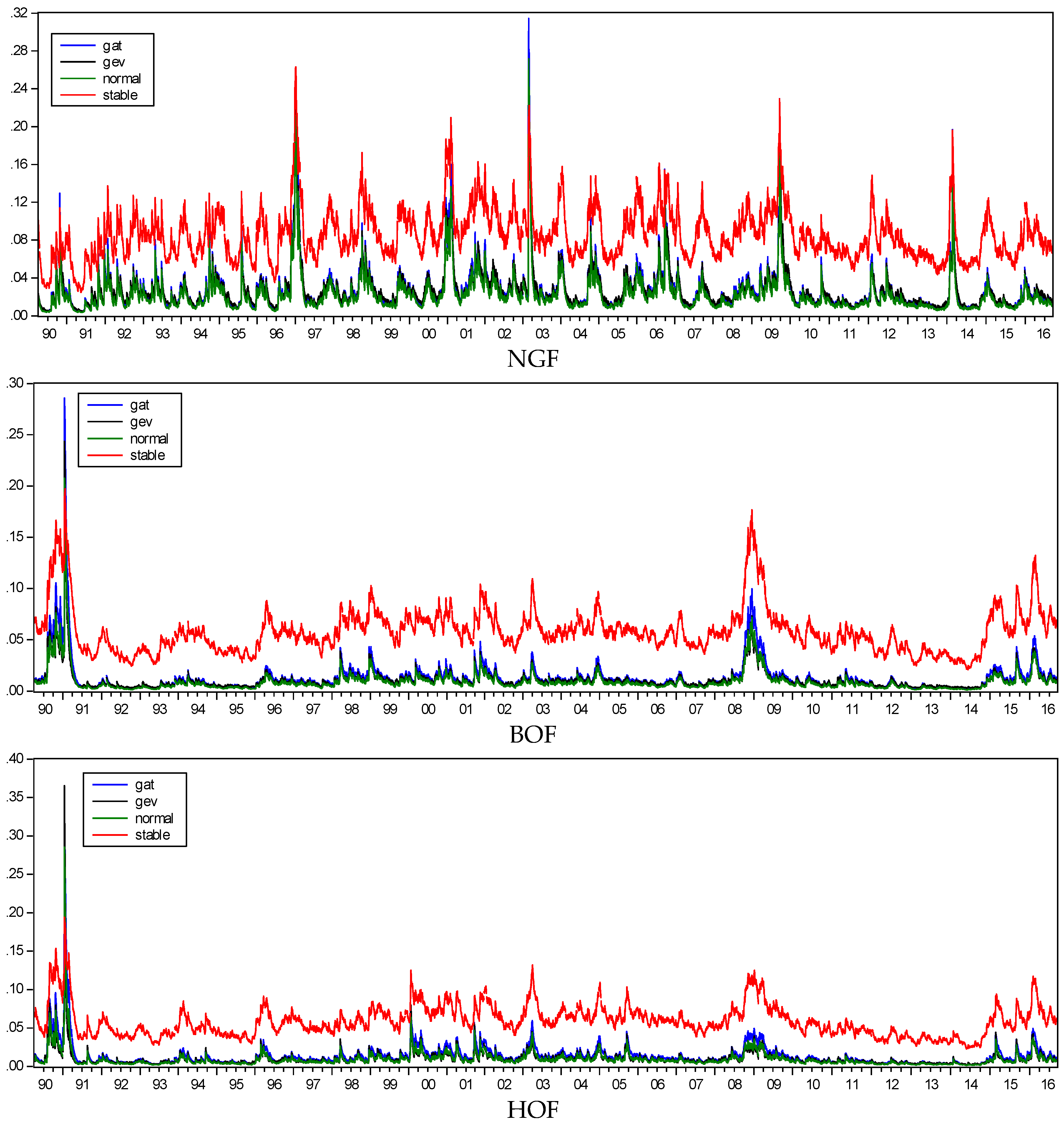
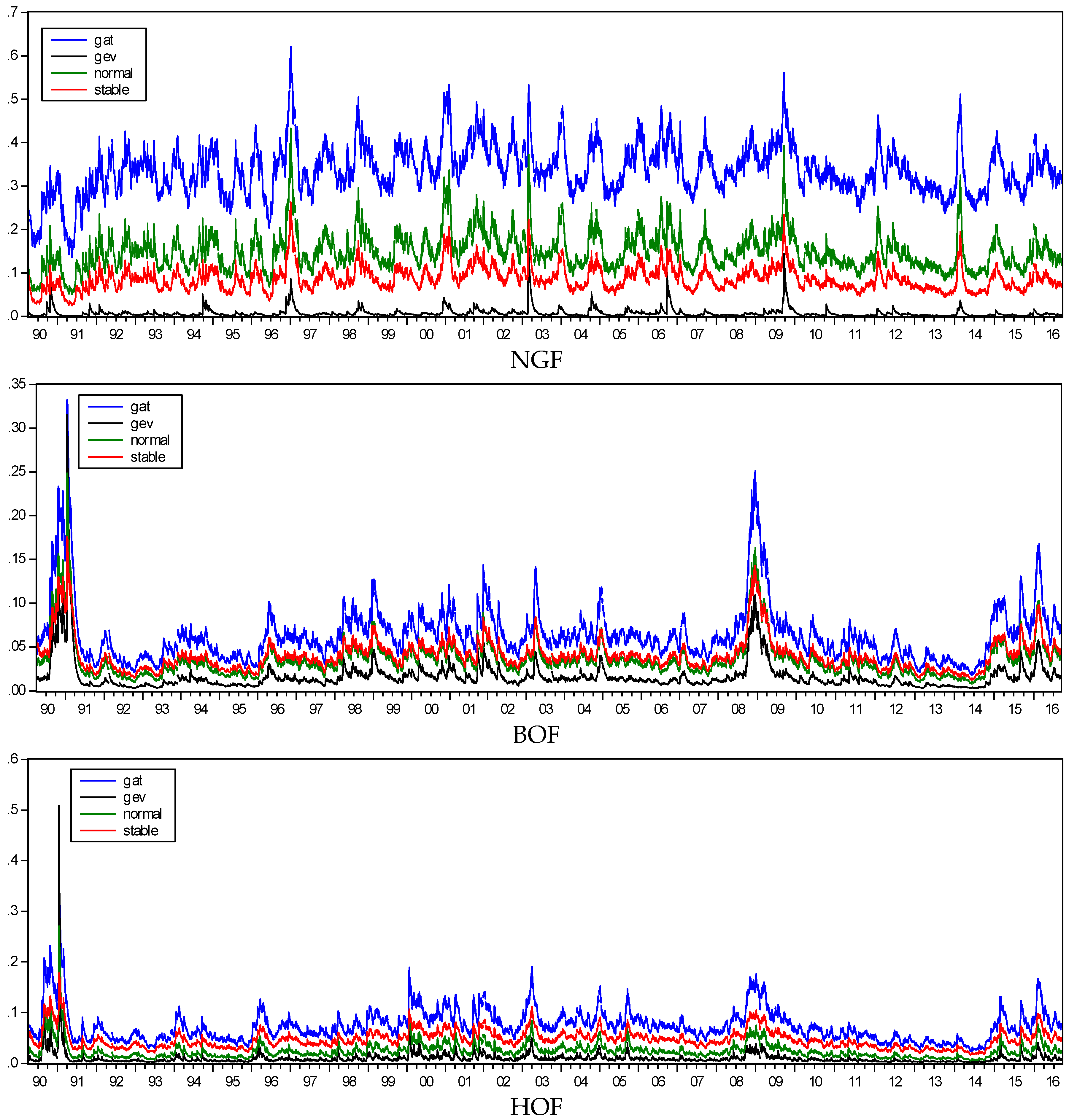
4.3. Volatility Modeling—GARCH (1.1) and APARCH (1.1)
5. Conclusions
Author Contributions
Conflicts of Interest
References
- Agnolucci, Paolo. 2009. Volatility in crude oil futures: A comparison of the predictive ability of GARCH and implied volatility models. Energy Economics 31: 316–21. [Google Scholar] [CrossRef]
- Ahmed, Elsheikh M., and Suliman Zakaria. 2011. Modeling stock market volatility using GARCH models evidence from Sudan. International Journal of Business and Social Science, 4. [Google Scholar] [CrossRef]
- Aloui, Chaker, and Rania Jammazi. 2009. The effects of crude oil shocks on stock market shifts behaviour: A regime switching approach. Energy Economics 31: 789–99. [Google Scholar] [CrossRef]
- Aloui, Chaker, and Samir Mabrouk. 2010. Value-at-risk estimations of energy commodities via long-memory, asymmetry and fat-tailed GARCH models. EnergyPolicy 38: 2326–39. [Google Scholar] [CrossRef]
- Alvarez-Ramirez, Jose, Myriam Cisneros, Carlos Ibarra-Valdez, and Angel Soriano. 2002. Multifractal Hurst analysis of crude oil prices. Physica A: Statistical Mechanics and Its Applications 313: 651–70. [Google Scholar] [CrossRef]
- Bali, Turan G. 2003. An extreme value approach to estimating volatility and value at risk. The Journal of Business 76: 83–108. [Google Scholar] [CrossRef]
- Bali, Turan G. 2007. A generalized extreme value approach to financial risk measurement. Journal of Money, Credit and Banking 39: 1613–49. [Google Scholar] [CrossRef]
- Billio, Monica, and Loriano Pelizzon. 2000. Value-at-risk: a multivariate switching regime approach. Journal of Empirical Finance 7: 531–54. [Google Scholar] [CrossRef]
- Black, Fischer. 1976. Studies in Stock Price Volatility Changes. In Proceedings from the Business and Economics Statistics Section. Boston: American Statistical Association, pp. 177–81. [Google Scholar]
- Bollerslev, Tim. 1986. Generalized autoregressive conditional heteroskedasticity. Journal of Econometrics 31: 307–27. [Google Scholar] [CrossRef]
- Carl, Peter, and Brian G. Peterson. 2014. Package ‘Performance Analytics’. Available online: http://r-forge.r-project.org/projects/returnanalytics/ (accessed on 23 June 2017).
- Cartea, Alvaro, and Marcelo G. Figueroa. 2005. Pricing in electricity markets: A mean reverting jump diffusion model with seasonality. Applied Mathematical Finance 12: 313–35. [Google Scholar] [CrossRef] [Green Version]
- Cartea, Álvaro, and Pablo Villaplana. 2008. Spot price modeling and the valuation of electricity forward contracts: The role of demand and capacity. Journal of Banking & Finance 32: 2502–19. [Google Scholar]
- Cheong, Chin Wen. 2009. Modeling and forecasting crude oil markets using ARCH-type models. Energy Policy 37: 2346–55. [Google Scholar] [CrossRef]
- Chkili, Walid, Shawkat Hammoudeh, and Duc Khuong Nguyen. 2014. Volatility forecasting and risk management for commodity markets in the presence of asymmetry and long memory. Energy Economics 41: 1–18. [Google Scholar] [CrossRef]
- Christie, Andrew A. 1982. The stochastic behavior of common stock variances: Value, leverage and interest rate effects. Journal of Financial Economics 10: 407–32. [Google Scholar] [CrossRef]
- Cont, Rama. 2001. Empirical properties of asset returns: Stylized facts and statistical issues. Quantitative Finance 1: 223–36. [Google Scholar] [CrossRef]
- Cortazar, Gonzalo, and Eduardo S. Schwartz. 1994. The valuation of commodity contingent claims. The Journal of Derivatives 1: 27–39. [Google Scholar] [CrossRef]
- Ding, Zhuanxin, Clive W. Granger, and Robert F. Engle. 1993. A long memory property of stock market returns and a new model. Journal of Empirical Finance 1: 83–106. [Google Scholar] [CrossRef]
- Engle, Robert F. 1982. Autoregressive conditional heteroscedasticity with estimates of the variance of United Kingdom inflation. Econometrica: Journal of the Econometric Society 50: 987–1007. [Google Scholar] [CrossRef]
- Engle, Robert F. 1990. Discussion: stock market volatility and the crash. Review of Financial Studies 3: 103–6. [Google Scholar] [CrossRef]
- Engle, Robert F., Neil Shephard, and Kevin Sheppard. 2007. Fitting and Testing Vast Dimensional Time-Varying Covariance Models. NYU Working Paper No. FIN-07-046. Available online: https://ssrn.com/abstract=1293629 (accessed on 27 May 2017).
- Eydeland, Alexander, and Krzysztof Wolyniec. 2003. Energy and Power Risk Management: New Developments in Modeling, Pricing, and Hedging (Vol. 206). Hoboken: John Wiley & Sons. [Google Scholar]
- Fan, Ying, Yue-Jun Zhang, Hsein-Tang Tsai, and Yi-Ming Wei. 2008. Estimating ‘Value at Risk’of crude oil price and its spillover effect using the GED-GARCH approach. Energy Economics 30: 3156–71. [Google Scholar] [CrossRef]
- Feng, L., and Y. Shi. 2017. Fractionally integrated garch model with tempered stable distribution: A simulation study. Journal of Applied Statistics 44: 2837–57. [Google Scholar] [CrossRef]
- Gibson, Rajna, and Eduardo S. Schwartz. 1990. Stochastic convenience yield and the pricing of oil contingent claims. The Journal of Finance 45: 959–76. [Google Scholar] [CrossRef]
- Giot, Pierre, and Sebastien Laurent. 2003. Market risk in commodity markets: A VaR approach. Energy Economics 25: 435–57. [Google Scholar] [CrossRef]
- Glosten, Lawrence R., Ravi Jagannathan, and David E. Runkle. 1993. On the relation between the expected value and the volatility of the nominal excess return on stocks. The Journal of Finance 48: 1779–801. [Google Scholar] [CrossRef]
- Gnedenko, Par B. 1943. Sur la distribution limite du terme maximum d’uneseriealeatoire. Annals of Mathematics 44: 423–53. [Google Scholar] [CrossRef]
- Gunay, Samet. 2015. Markov Regime Switching GARCH Model and Volatility Modeling for Oil Returns. International Journal of Energy Economics and Policy 5: 979–85. [Google Scholar]
- Hansen, Bruce E. 1994. Autoregressive conditional density estimation. International Economic Review 35: 705–30. [Google Scholar] [CrossRef]
- Huang, Yu Chuan, and Bor-Jing Lin. 2004. Value-at-risk analysis for Taiwan stock index futures: Fat tails and conditional asymmetries in return innovations. Review of Quantitative Finance and Accounting 22: 79–95. [Google Scholar] [CrossRef]
- Hung, Jui-Cheng, Ming-Chih Lee, and Hung-Chun Liu. 2008. Estimation of value-at-risk for energy commodities via fat-tailed GARCH models. Energy Economics 30: 1173–91. [Google Scholar] [CrossRef]
- Jackwerth, Jens Carsten, and Mark Rubinstein. 1996. Recovering probability distributions from option prices. The Journal of Finance 51: 1611–31. [Google Scholar] [CrossRef]
- Jenkinson, Arthur F. 1955. The frequency distribution of the annual maximum (or minimum) values of meteorological elements. Quarterly Journal of the Royal Meteorological Society 81: 158–71. [Google Scholar] [CrossRef]
- Kanamura, Takashi. 2009. A supply and demand based volatility model for energy prices. Energy Economics 31: 736–47. [Google Scholar] [CrossRef]
- Kang, Sang Hoon, Sang-Mok Kang, and Seong-Min Yoon. 2009. Forecasting volatility of crude oil markets. Energy Economics 31: 119–25. [Google Scholar] [CrossRef]
- Kapetanios, George. 2005. Unit-root testing against the alternative hypothesis of up to m structural breaks. Journal of Time Series Analysis 26: 123–33. [Google Scholar] [CrossRef]
- Knittel, Christopher R., and Michael R. Roberts. 2005. An empirical examination of restructured electricity prices. Energy Economics 27: 791–817. [Google Scholar] [CrossRef]
- Kristoufek, Ladislav. 2014. Leverage effect in energy futures. Energy Economics 45: 1–9. [Google Scholar] [CrossRef] [Green Version]
- Laurent, Sebastien. 2004. Analytical derivates of the APARCH model. Computational Economics 24: 51–57. [Google Scholar] [CrossRef]
- Mandelbrot, Benoit. 1972. Statistical methodology for nonperiodic cycles: From the covariance to R/S analysis. Annals of Economic and Social Measurement 1: 259–90. [Google Scholar]
- Markose, Sheri, and Amadeo Alentorn. 2011. The generalized extreme value distribution, implied tail index, and option pricing. The Journal of Derivatives 18: 35–60. [Google Scholar] [CrossRef]
- Mohammadi, Hassan, and Lixian Su. 2010. International evidence on crude oil price dynamics: Applications of ARIMA-GARCH models. Energy Economics 32: 1001–8. [Google Scholar] [CrossRef]
- Nelson, Daniel B. 1991. Conditional heteroskedasticity in asset returns: A new approach. Econometrica: Journal of the Econometric Societ 59: 347–70. [Google Scholar] [CrossRef]
- Nolan, John P. 2005. Modeling Financial Data with Stable Distributions. Washington: Department of Mathematics and Statistics, American University. [Google Scholar]
- Nomikos, Nikos, and Kostas Andriosopoulos. 2012. Modelling energy spot prices: Empirical evidence from NYMEX. Energy Economics 34: 1153–69. [Google Scholar] [CrossRef]
- Panas, Epaminondas. 2001. Estimating fractal dimension using stable distributions and exploring long memory through ARFIMA models in Athens Stock Exchange. Applied Financial Economics 11: 395–402. [Google Scholar] [CrossRef]
- Reiss, R.D., and M. Thomas. 2001. Statistical Analysis of Extreme Values: With Applications to Insurance, Finance, Hydrology, and Other Fields. Basel, Boston and Berlin: Birkhäuser. [Google Scholar]
- Sadorsky, Perry. 2006. Modeling and forecasting petroleum futures volatility. Energy Economics 28: 467–88. [Google Scholar] [CrossRef]
- Sáfadi, Thelma, and Airlane P. Alencar. 2014. Volatility and Returns of the Main Stock Indices. In New Advances in Statistical Modeling and Applications. Basel: Springer International Publishing, pp. 229–37. [Google Scholar]
- Schwartz, Eduardo S. 1997. The stochastic behavior of commodity prices: Implications for valuation and hedging. The Journal of Finance 52: 923–73. [Google Scholar] [CrossRef]
- Schwert, G.William. 1989. Why does stock market volatility change over time? The Journal of Finance 44: 1115–53. [Google Scholar] [CrossRef]
- Sentana, Enrique. 1991. Quadratic ARCH Models: A Potential Reinterpretation of ARCH Models as Second-Order Taylor Approximations. London: London School of Economics and Political Science, Unpublished paper. [Google Scholar]
- Serletis, Apostolos, and Ioannis Andreadis. 2004. Random fractal structures in North American energy markets. Energy Economics 26: 389–99. [Google Scholar] [CrossRef]
- Sheikh, Aamir M. 1991. Transaction data tests of S&P 100 call option pricing. Journal of Financial and Quantitative Analysis 26: 459–75. [Google Scholar]
- Sousa, Thiago, Cira Otiniano, Silvia Lopes, and Diethelm Wuertz. 2015. Package ‘GEVStableGarch’. Available online: https://CRAN.R-project.org/package=GEVStableGarch (accessed on 05 June 2017).
- Taleb, Nassim Nicholas. 2007. The Black Swan: The Impact of the Highly Improbable. New York: Random. [Google Scholar]
- Taylor, Stephen J. 1986. Modelling Financial Time Series. New York: John Wiley & Sons. [Google Scholar]
- Wei, Yu, Yudong Wang, and Dengshi Huang. 2010. Forecasting crude oil market volatility: Further evidence using GARCH-class models. Energy Economics 32: 1477–84. [Google Scholar] [CrossRef]
- Weron, Rafal. 2001. Levy-stable distributions revisited: Tail index > 2 does not exclude the Levy-stable regime. International Journal of Modern Physics 12: 209–23. [Google Scholar] [CrossRef]
- Zhang, Xun, K.K. Lai, and Shou-Yang Wang. 2008. A new approach for crude oil price analysis based on Empirical Mode Decomposition. Energy Economics 30: 905–18. [Google Scholar] [CrossRef]
- Zakoian, Jean-Michel. 1994. Threshold heteroskedastic models. Journal of Economic Dynamics and Control 18: 931–55. [Google Scholar] [CrossRef]
- Zhu, Dongming, and John W Galbraith. 2010. A generalized asymmetric Student-t distribution with application to financial econometrics. Journal of Econometrics 157: 297–305. [Google Scholar] [CrossRef]
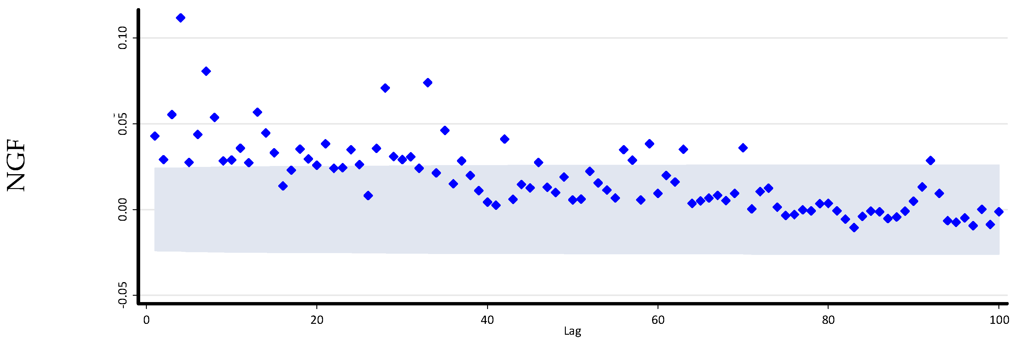
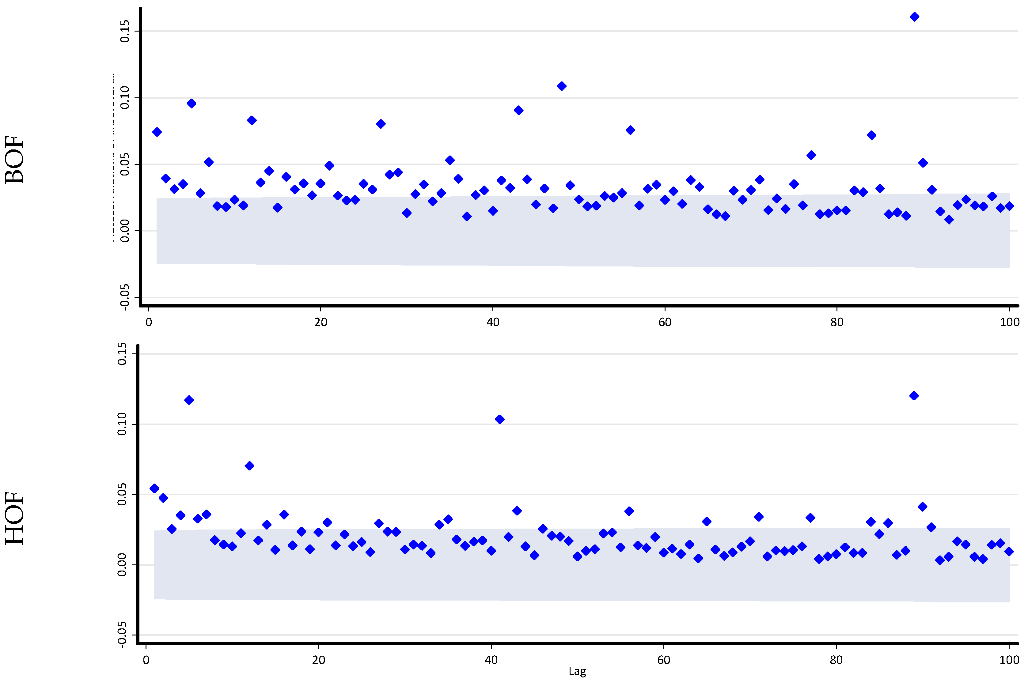
| 1 | (Kolmogorov-Smirnov) test. |


| Variables | NGF | BOF | HOF |
|---|---|---|---|
| t statistic | −83.8434 *** | −61.2692 *** | −59.9970 *** |
| Break Dates | 22.10.1990 22.01.1991 2.07.2008 4.08.2009 20.10.2009 | 26.09.1990 17.01.1991 1.04.2015 21.08.2015 19.01.2016 | 22.08.1990 28.02.1991 25.08.2015 19.01.2016 4.04.2016 |
| Anderson-Darling | Cramer-Von Mises | Lilliefors1 | Pearson Chi-Square | |
|---|---|---|---|---|
| NGF | 58.1037 | 9.6436 | 0.0603 | 966.7539 |
| BOF | 57.0350 | 9.8300 | 0.0595 | 586.6152 |
| HOF | 47.7956 | 8.0555 | 0.0567 | 532.1663 |
| p | <2.2 × 10⁻¹⁶ | =7.37 × 10⁻¹⁰ | <2.2 × 10⁻¹⁶ | <2.2 × 10⁻¹⁶ |
| NGF | BOF | HOF | |
|---|---|---|---|
| Alpha | 1.7088 | 1.7070 | 1.73878 |
| Beta | 0.0596 | −0.0774 | 0.00143 |
| Gamma | 0.0081 | 0.0054 | 0.00558 |
| Delta | 3.0350 | 6.3992 | 0.00013 |
| NGF | BOF | HOF | ||||||||||
|---|---|---|---|---|---|---|---|---|---|---|---|---|
| Normal | Gev | Gat | Stable | Normal | Gev | Gat | Stable | Normal | Gev | Gat | Stable | |
| 0.0013 (0.0015) | −0.046 *** (0.0020) | −0.0032 (0.0023) | −0.0018 (0.0015) | 0.0008 (0.0009) | −0.021 *** (0.0016) | 0.0045 *** (0.001548) | 0.0028 *** (0.0010) | 0.0006 (0.0018) | −0.024 *** (0.0011) | 0.0003 (0.0016) | 0.0015 (0.0011) | |
| 0.0003 *** (0.0001) | 0.0002 *** (0.0001) | 0.0003 *** (0.0001) | 0.0012 *** (0.0003) | 0.0000 *** (0.0000) | 0.0002* (0.0001) | 0.0001 *** (0.0000) | 0.0003 *** (0.0001) | 0.0001 (0.0001) | 0.0001 *** (0.0000) | 0.0001 *** (0.0000) | 0.0004 *** (0.0001) | |
| 0.0866 *** (0.0077) | 0.0756 *** (0.0045) | 0.0993 *** (0.0098) | 0.0562 *** (0.0046) | 0.0615 *** (0.0053) | 0.0766 *** (0.0113) | 0.0840 *** (0.0093) | 0.0408 *** (0.0036) | 0.0800*** (0.0120) | 0.1082*** (0.0075) | 0.0930*** (0.0103) | 0.0415*** (0.0040) | |
| 0.9074*** (0.0070) | 0.9301*** (0.0041) | 0.9116*** (0.0074) | 0.9189** (0.0066) | 0.9361*** (0.0053) | 0.9145*** (0.0215) | 0.9375*** (0.0061) | 0.9471*** (0.0047) | 0.9145*** (0.0071) | 0.8733*** (0.0094) | 0.9324*** (0.0071) | 0.9452*** (0.0055) | |
| 1.0221*** (0.0142) | 0.1846*** (0.0732) | 0.9659*** (0.0136) | −0.309*** (0.1009) | 1.0046*** (0.0141) | −0.0775 (0.0988) | |||||||
| −0.119 *** (0.0014) | 2.7817 *** (0.4677) | 1.8237 *** (0.0188) | −0.25 *** (0.0060) | 5.4139 *** (1.4192) | 1.8843 *** (0.0166) | −0.222 *** (0.0037) | 3.4654 *** (0.7434) | 1.8830 *** (0.0161) | ||||
| 1.9682 *** (0.1143) | 1.8181 *** (0.1065) | 2.047 *** (0.1265) | ||||||||||
| −2LLH | −3937.731 | −3328.229 | −4267.178 | −4316.006 | −7060.604 | −6596.071 | −7189.15 | −7174.745 | −6927.728 | −6631.949 | −7044.126 | −7044.521 |
| AIC | −7867.024 | −6646.581 | −8519.839 | −8619.349 | −14,113.21 | −13,182.14 | −14,364.30 | −14,337.49 | −13,847.46 | −13,253.90 | −14,074.25 | −14,077.04 |
| BIC | −7839.797 | −6612.548 | −8472.192 | −8578.509 | −14,085.98 | −13,148.11 | −14,316.65 | −14,296.65 | −13,820.23 | −13,219.86 | −14,026.61 | −14,036.20 |
| AICc | −7865.015 | −6644.569 | −8517.818 | −8617.332 | −14,111.20 | −13,180.13 | −14,362.28 | −14,335.47 | −13,845.45 | −13,251.88 | −14,072.23 | −14,075.03 |
| NGF | BOF | HOF | ||||||||||
|---|---|---|---|---|---|---|---|---|---|---|---|---|
| Normal | Gev | Gat | Stable | Normal | Gev | Gat | Stable | Normal | Gev | Gat | Stable | |
| 0.0012 (0.0014) | −0.048 *** (0.0019) | 0.0000 (0.0000) | −0.0015 (0.0111) | 0.0005 (0.0010) | −0.025 *** (0.0011) | 0.0036** (0.0017) | 0.0020** (0.0010) | 0.0012 (0.0010) | −0.026 *** (0.0012) | 0.0008 (0.0018) | 0.0014 (0.0009) | |
| 0.0033 *** (0.0009) | 0.0000 (0.0000) | 0.0067 *** (0.0017) | 0.0012 (0.0090) | 0.0002** (0.0000) | 0.0001 *** (0.0000) | 0.0003** (0.0002) | 0.00020** (0.0001) | 0.0002 *** (0.0001) | 0.0002 *** (0.0001) | 0.0005** (0.0002) | 0.0003** (0.0001) | |
| 0.09466 *** (0.0067) | 0.0305 *** (0.0046) | 0.0830 *** (0.0076) | 0.0560** (0.0230) | 0.0640 *** (0.0054) | 0.0756 *** (0.0041) | 0.0773 *** (0.0073) | 0.0366 *** (0.0036) | 0.0840 *** (0.0074) | 0.1305 *** (0.0070) | 0.08467 *** (0.0083) | 0.0404 *** (0.0042) | |
| 0.9090 *** (0.0068) | 0.9356 *** (0.0044) | 0.9214 *** (0.0064) | 0.9189 *** (0.0650) | 0.9439 *** (0.0051) | 0.9400 *** (0.0041) | 0.9460 *** (0.0050) | 0.9497 *** (0.0049) | 0.9206 *** (0.0070) | 0.8626 *** (0.0069) | 0.9413 *** (0.0057) | 0.9445 *** (0.0055) | |
| −0.0926** (0.0365) | −0.286 *** (0.0510) | −0.0794 (0.0527) | −0.0502 (0.4454) | 0.1048** (0.0438) | 0.1976 *** (0.0135) | 0.1505** (0.0587) | 0.2062 (0.0624) | −0.0647** (0.0330) | 0.0993 *** (0.0168) | −0.0031 (0.0517) | 0.0112 (0.0528) | |
| 0.9640 *** (0.0962) | 2.8149 *** (0.1911) | 0.5787 *** (0.0633) | 1.0000 (3.0099) | 1.3974 *** (0.1322) | 1.8243 *** (0.0089) | 1.2334 *** (0.1445) | 1.1356 *** (0.1235) | 1.5676 *** (0.1191) | 2.0290 *** (0.1250) | 1.1864 *** (0.1356) | 1.0838 *** (0.1259) | |
| 1.0032 *** (0.0076) | 0.1769 (0.1973) | 0.9718 *** (0.0146) | −0.273 *** (0.1006) | 1.0011 *** (0.0153) | −0.0729 (0.0989) | |||||||
| −0.12 *** (0.0014) | 2.1095 *** (0.3051) | 1.8245 *** (0.0538) | −0.212 *** (0.0023) | 4.7745 *** (1.1761) | 1.8881 *** (0.0164) | −0.224 *** (0.0029) | 3.0279 *** (0.5491) | 1.8836 *** (0.0164) | ||||
| 2.1964 *** (0.1253) | 1.8703 *** (0.1129) | 2.1325 *** (0.1261) | ||||||||||
| −2LLH | −3979.801 | −3360.967 | −4348.198 | −4316.172 | −7070.074 | −6678.638 | −7201.241 | −7184.251 | −6936.185 | −6645.672 | −7059.333 | −7044.807 |
| AIC | −7947.603 | −6707.935 | −8678.396 | −8616.344 | −14,128.15 | −13,343.28 | −14,384.48 | −14,352.50 | −13,860.37 | −13,277.34 | −14,100.67 | −14,073.61 |
| BIC | −7906.762 | −6660.288 | −8617.136 | −8561.890 | −14,087.31 | −13,295.63 | −14,323.22 | −14,298.05 | −13,819.53 | −13,229.70 | −14,039.40 | −14,019.16 |
| AICc | −7945.586 | −6705.913 | −8676.363 | −8614.317 | −14,126.13 | −13,341.25 | −14,382.45 | −14,350.48 | −13,858.35 | −13,275.32 | −14,098.63 | −14,071.59 |
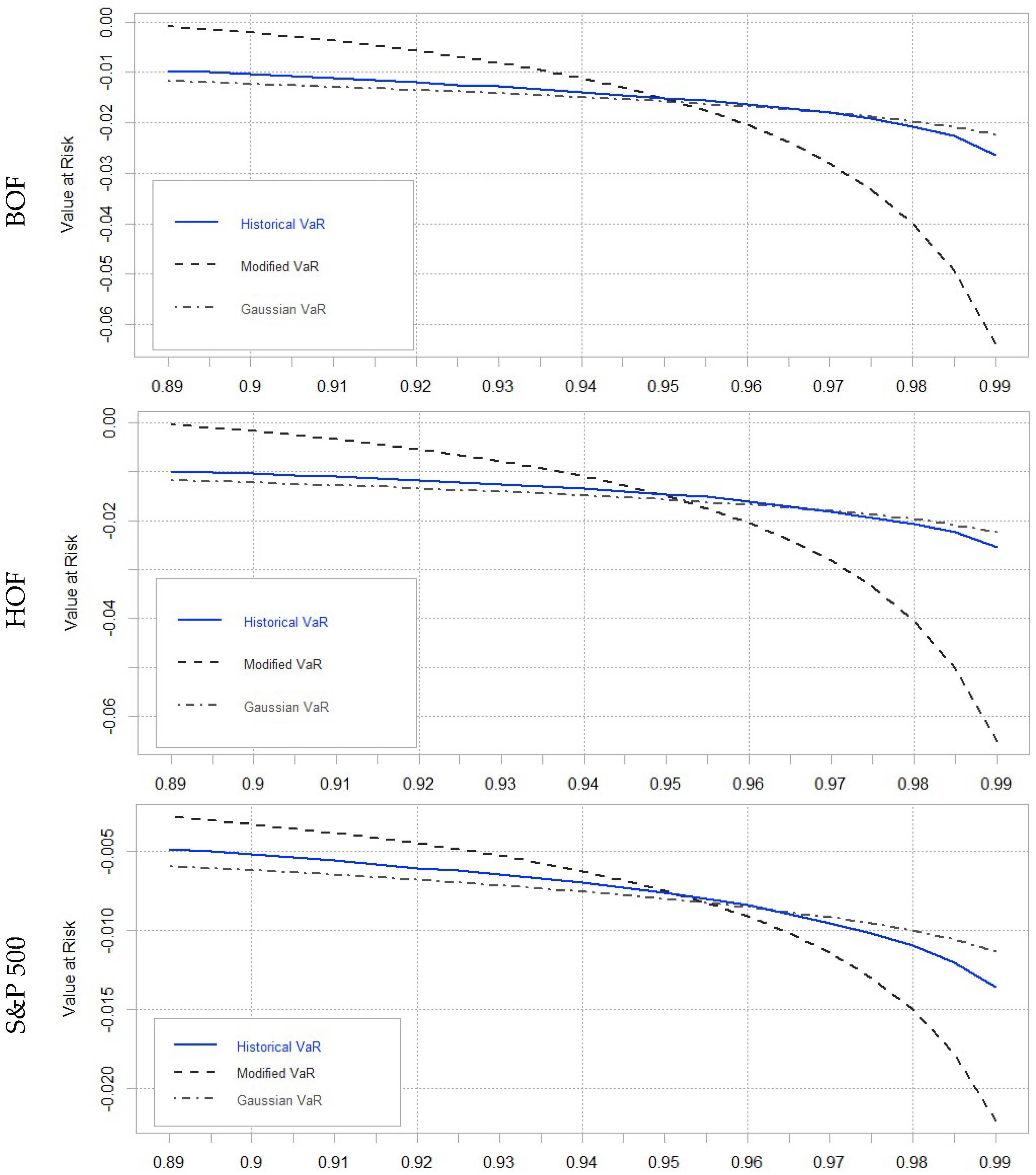
| Gaussian VaR | Historical VaR | Modified VaR | |
|---|---|---|---|
| NGF | −0.0237 | −0.0216 | −0.0206 |
| BOF | −0.0158 | −0.0151 | −0.0151 |
| HOF | −0.0158 | −0.0148 | −0.0150 |
| S&P 500 | −0.0080 | −0.0076 | −0.0075 |
© 2018 by the authors. Licensee MDPI, Basel, Switzerland. This article is an open access article distributed under the terms and conditions of the Creative Commons Attribution (CC BY) license (http://creativecommons.org/licenses/by/4.0/).
Share and Cite
Gunay, S.; Khaki, A.R. Best Fitting Fat Tail Distribution for the Volatilities of Energy Futures: Gev, Gat and Stable Distributions in GARCH and APARCH Models. J. Risk Financial Manag. 2018, 11, 30. https://doi.org/10.3390/jrfm11020030
Gunay S, Khaki AR. Best Fitting Fat Tail Distribution for the Volatilities of Energy Futures: Gev, Gat and Stable Distributions in GARCH and APARCH Models. Journal of Risk and Financial Management. 2018; 11(2):30. https://doi.org/10.3390/jrfm11020030
Chicago/Turabian StyleGunay, Samet, and Audil Rashid Khaki. 2018. "Best Fitting Fat Tail Distribution for the Volatilities of Energy Futures: Gev, Gat and Stable Distributions in GARCH and APARCH Models" Journal of Risk and Financial Management 11, no. 2: 30. https://doi.org/10.3390/jrfm11020030