How Informative Are Earnings Forecasts? ^†

Abstract

We constructed forecasts of earnings forecasts using data on 406 firms and forecasts made by 5419 individuals with on average 25 forecasts per individual. We verified previously found predictors, which are the average of the most recent available forecast for each forecaster and the difference between the average and the forecast that this forecaster previously made. We extended the knowledge base by analyzing the unpredictable component of the earnings forecast. We found that for some forecasters the unpredictable component can be used to improve upon the predictable forecast, but we also found that this property is not persistent over time. Hence, a user of the forecasts cannot trust that the forecaster will remain to be of forecasting value. We found that, in general, the larger is the unpredictable component, the larger is the forecast error, while small unpredictable components can lead to gains in forecast accuracy. Based on our results, we formulate the following practical guidelines for investors: (i) for earnings analysts themselves, it seems to be the safest to not make large adjustments to the predictable forecast, unless one is very confident about the additional information; and (ii) for users of earnings forecasts, it seems best to only use those forecasts that do not differ much from their predicted values.

1. Introduction

Earnings forecasts can provide useful information for investors. When investors in part rely on such forecasts, it is important to have more insights into how such earnings forecasts are created. A key research subject therefore concerns the drivers of the forecasts of earnings analysts. Such knowledge is relevant as the part that can be predicted from factors that are also observable to the end user of the forecast might not be the most interesting part of an earnings forecast. Indeed, it is the unpredictable component of the earnings forecast that amounts to the forecaster’s true added value, based on latent expertise and domain-specific knowledge. Consequently, in our perspective, the evaluation of the quality of earnings forecasts should mainly focus on that unpredictable part, as that is truly the added value of the professional forecaster.

There is much literature on the properties and accuracy of earnings forecasts, but there is no research that focuses on the prediction of such forecasts. Which variables are the most relevant drivers of earnings forecasts? Can we use the unpredictable part of the forecast to improve forecasts? In this paperm we answer these questions using appropriate models. We applied these models to the earnings forecasts for a large number of firms which constitute the S&P500. Using this large sample of firms, we are confident to draw a few generalizing conclusions.

A key predictor of the earnings forecasts appears to be the average of all available earnings forecasts concerning the same forecast event. As an example, consider a forecaster who has produced his most recent forecast some time ago. If in the meantime information has been provided on the firm that has driven the forecasts of all (other) forecasters down, this forecaster will also on average produce a lower-valued forecast than before. A second predictor is the most recent difference between the individual forecaster’s forecast and the average of the available contemporaneous forecasts. For example, a forecaster who previously was more optimistic about the earnings of a particular firm can be expected to persist in quoting above-average values. Other important conclusions that we draw from the data are that more unpredictable forecasts tend to be less accurate, and that the unpredictable component of the forecast can be used to improve the forecast. Overall, we document that earnings forecasts are quite predictable from data that are also available to the end user.

The outline of our paper is as follows. In Section 2, we develop several hypotheses to guide our empirical analysis, and we base these hypotheses on available studies, reviewed in Section 2. In Section 3, we discuss the data and, in Section 4 and Section 5, we present our results. Section 6 concludes and provides various avenues for further research.

2. Literature Review

Earnings forecasts have been the topic of interest for many researchers. For an extensive discussion of research on earnings forecasts in the period 1992–2007, see Ramnath et al. (2008). For earlier overviews, we refer to Schipper (1991) and Brown (1993).

One stream of earnings forecasts research has focused on relationships between forecast performance and forecaster characteristics. Performance can be measured by forecast accuracy and forecast impact on stock market fluctuations. The characteristics of these performance measurements have been related to timeliness (Cooper et al. 2001; Kim et al. 2011), the number of firms that the analyst follows (Bolliger 2004; Kim et al. 2011), the firm-specific experience of the analyst (Bolliger 2004), age (Bolliger 2004), the size of the firm being followed and of the firm at which the analyst works (Bolliger 2004; Kim et al. 2011), and whether the analyst works individually or in a team (Brown and Hugon 2009).

Another stream of research concerns the value of an earnings forecast and how it is related to what other analysts do. In particular, herding behavior is considered, which occurs when forecasters produce forecasts that converge towards the average of those of the other forecasters. There has been an effort to categorize earnings forecasters into two groups, corresponding to leaders and followers or to innovators and herders (Clement and Tse 2005; Jegadeesh and Woojin 2010). This is interesting as different types of forecasters might consult different amounts of information which in turn can be useful for investors to incorporate into their investment decisions. A leading or innovating forecaster might on average be more useful to follow than a herding forecaster. This does not directly imply that leading forecasts are also more accurate, as accuracy and the type of forecast are not necessarily related. In fact, it has been documented that aggregation of leading forecasts is a fruitful tactic to produce accurate forecasts (Kim et al. 2011).

Recently, Clement et al. (2011) studied the effect of stock returns and other analysts’ forecasts on what analysts do. In contrast to Jegadeesh and Woojin (2010) and Clement and Tse (2005), Clement et al. (2011) did not consider categorizing the forecasters into different groups. Instead, they considered how the first forecast revision after a forecast announcement is affected by how the stock market and other analysts have reacted to that forecast announcement. Landsman et al. (2012) also looked at how earnings announcements affect the stock market, focusing on how mandatory IFRS adoption has influenced this effect. Sheng and Thevenot (2012) proposed a new earnings forecast uncertainty measure, which they use to demonstrate that forecasters focus more on the information in the earnings announcement if there is high uncertainty in the available set of earnings forecasts.

In sum, earnings forecasts have been studied concerning their performance and a few of their potential drivers. In this paper, we extend the knowledge base by considering many more drivers of earnings forecasts, while we pay specific attention to the value of the unpredictable component of earnings forecasts.

3. Data and Sample Selection

Data were collected from WRDS1, using the I/B/E/S database for the analyst forecasts and the CRSP data for the stock prices and returns.

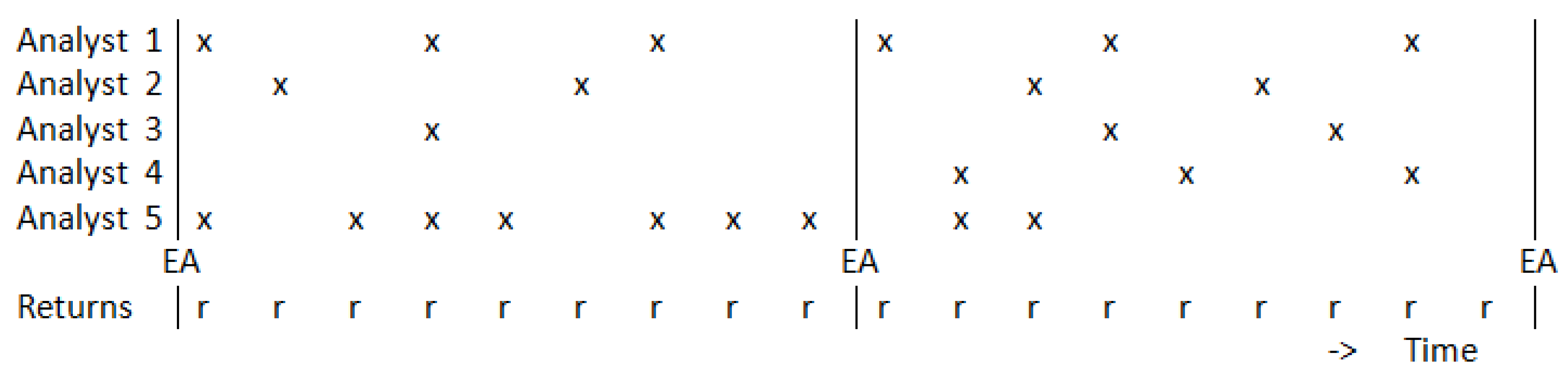
Concerning the earnings forecasts, we collected data for all firms which have been part of the S&P500 during the period 1995–2011. This amounts to 658 firms due to mergers, name changes and entry and exit of firms. We focused on the within-year yearly earnings forecasts, that is, the forecasts that are produced to forecast the earnings of the current year. The structure of the data is characterized in Figure 1. This figure shows a cross for the moment an analyst makes a forecast available, which is not at the same moment or with the same frequency for all analysts. Next, this figure shows that there are variables which we measured at the highest frequency. As an example, the returns are shown, which we measured daily. Finally, this figure shows vertical lines depicting the moment of the earnings announcement, at which point the realization occurs of the variable that is to be forecasted by the analysts. We only used within-year earnings forecasts, which means that we only included forecasts that are forecasting the variable announced at the next upcoming yearly earnings announcement.

For several reasons, we had to omit some of the data at different parts of the rest of the paper. For example, we linked the earnings data to the stock data where possible, but for some firms this link could not be established. In addition, we had a threshold for the number of observations that we wanted at minimum for each regression or correlation. For these reasons and other, smaller reasons, the initial sample was cut down to 316 firms. Some descriptives of the remaining sample are shown in

Table 1. The number of firms, forecasters and forecasts for each upcoming section and subsection. The number of forecasts is shown separately for the estimation sample, which is up until 2005, and the evaluation sample, which is from 2006 onwards.

	Number of Firms	Number of Forecasters	Number of Forecasts
			Estimation Sample	Evaluation Sample
Section 4 and Section 5.1	316	18,338	146,319	126,651
Section 5.2	316	1835	52,236	36,403
Section 5.3	316	4541	90,190	28,000

. The large drop in number of forecasters and forecasts in Section 5.2 and Section 5.3 are due to the fact that we used forecaster-specific regressions and correlations in these sections, meaning that the majority of forecasters (those with only a few observations) dropped out.

4. Predicting Earnings Forecasts

In this section, we put forward a model to predict earnings forecasts using information available up until the day before the publication of the earnings forecast. First, we introduce the prediction equation that we used to predict the earnings forecast, and the variables that were included, for which we give estimation results. Next, we also discuss and apply a correction to account for the firms with a low number of observations.

4.1. The Prediction Equation, the Choice of Predictors and Estimation Results

For predicting the earnings forecast, we utilized a linear equation. In contrast to Stickel (1990), we were not interested in the change in the earnings forecast compared to the previous forecast, but focused on the earnings forecast directly. The set of predictors consists of several variables that were also used by Stickel (1990), as well as others. The full list of predictors can be found in

Table 2. The variables that were used to forecast the earnings forecast. These variables enter a linear model. They all use one-day lagged information. Several variables are based on historic analyst behaviour, while others are based on stock market data.

	Variable	Description
	Intercept
Analyst variables	Average Forecast	The average of all most recent forecasts of every forecaster, until the previous day
		Average Forecast is also included in a multiplication with two indicator variables:
		1. Whether the number of forecasters is lower than 10 or not
		2. Whether the time until the announcement of the earnings is more than two weeks or not
	$\mathsf{\Delta }$ Average Forecast	First difference in Average Active Forecast
	$\mathsf{\Delta }$ Previous Forecast	The difference between the previous forecast of the forecaster, and the average active forecast at that time
	Previous Forecast	The previous forecast of the individual forecaster
Stock variables	Stock Index Firm	The stock market index of the firm for which the earnings are forecasted
	Stock Returns Firm	The stock market daily returns of the firm for which the earnings are forecasted
	Cumulative Stock Returns Firm	Stock market returns of the firm since the day of the previous forecast by this forecaster
	Stock Index S&P500	The stock market index of the S&P500 index
	Stock Returns S&P500	The stock market daily returns of the S&P500 index
	Cumulative Stock Returns S&P500	Stock market returns of the S&P500 index since the day of the previous forecast by this forecaster

.

First, we expected forecasters to produce similar forecasts at similar times, both because they use roughly the same information to form the forecast and because they might even look at the values of competing forecasters. Thus, we used as predictor the average of all most recent forecasts per individual forecaster, in which we only included forecasts that have been made for the same year.

We also included several variables that are related to the average forecast. First, the average forecast might contain more information if it is based on a larger number of forecasters. To see whether this holds, we also include a cross product of the average forecast with an indicator function, that is 1 if the number of forecasters is below 10 and 0 otherwise. The average forecast might also be more relevant the closer we are to the announcement of the true value of the earnings. For this, we add a cross product with an indicator function for the last two weeks before the announcement. The final predictor related to the average forecast is the day-to-day growth. If the average forecast has risen on one day, that might cause individual forecasters to extrapolate this growth to the next day.

We also included several variables that are related to the stock market. First, we included the stock index of the firm for which these earnings are predicted, because stock market value might be related to earnings expectations, and this might not be entirely represented by the average forecast yet. In addition, recent increases in the stock market value might be a expected to continue according to an individual forecaster, so we also included stock market returns. We included two different returns: the daily return and the return relative to the previous time that individual produced a forecast. Next to these three firm-related stock market variables, we also included similar variables based on the entire S&P500 index.

Finally, we included two variables that are determined by the previous forecast of this forecaster. The first of these two is this previous forecast itself, and the other is the difference between this previous forecast and the average forecast at that time. These two variables allow for persistence in the opinion of the forecaster, for example if this forecaster is systematically more optimistic or pessimistic.

We estimated the prediction equation using Ordinary Least Squares for all firms, and aggregated estimation results across firms are shown in

Table 3. A summary of estimation results of forecasting earnings forecasts. Results are for the estimation sample, which amounts to 316 firms, 18.338 forecasters and 146.319 forecasts (on average slightly more than 463 forecasts per firm). As variable to be explained, we used the earnings forecasts by the analysts. As explanatory variables, we included the variables mentioned in Table 2. The regression was run individually for each firm, and the table shows statistics which summarize these results. The first five columns contain summary results on the regular parameter estimates (average, median, standard deviation and bounds of a 90% interval). The last three columns show summarized results for the standardized estimate, which is included to compare contributions to fit. The standardized estimate is defined as the estimate that would have been obtained had the regressor been standardized beforehand (which is a transformation to having an average of zero and a standard deviation of one).

		Estimate					Standardized Estimate
		Average	Median	Standard Deviation	Bounds of 90% Interval		Median	Median of Absolute	Contribution to Total Fit
	Intercept	−0.028	−0.026	0.278	−0.395	0.229
Analyst-based	Average Forecast	1.050	1.077	0.384	0.557	1.483	0.490	0.491	96.9%
	Average Forecast × $I[nrF<10]$	0.018	0.005	0.172	−0.053	0.078	0.001	0.004	0,0%
	Average Forecast × $I[TUA>14]$	−0.038	−0.034	0.292	−0.212	0.058	−0.017	0.025	0.3%
	$\mathsf{\Delta }$ Average Forecast	0.765	0.607	1.053	−0.526	2.438	0.005	0.006	0.0%
	$\mathsf{\Delta }$ Previous Forecast	0.498	0.548	0.359	−0.151	1.051	0.029	0.030	0.4%
	Previous Forecast	−0.046	−0.078	0.273	−0.388	0.375	−0.028	0.076	2.3%
Stock market	Stock Index Firm	0.002	0.001	0.004	−0.001	0.007	0.009	0.013	0.1%
	Stock Returns Firm	0.302	0.150	1.039	−0.264	1.291	0.005	0.007	0.0%
	Cumulative Stock Returns Firm	0.054	0.018	0.206	−0.092	0.285	0.003	0.005	0.0%
	Stock Index S&P500	0.000	0.000	0.002	−0.001	0.002	0.001	0.009	0.0%
	Stock Returns S&P500	−0.214	−0.096	1.226	-2.155	1.421	−0.001	0.004	0.0%
	Cumulative Stock Returns S&P500	−0.032	−0.006	0.238	−0.408	0.256	0.000	0.005	0.0%

. The first five columns show results on the aggregated raw estimate, including the mean, the median and the standard deviation of the estimates across all firms and also the 5% and 95% percentiles. The next two columns depict the aggregated standardized estimates, which are the estimates that are found if the variables are first all standardized. This measure can be helpful for comparing contribution to fit, as shown in the final column.

The results show that, on average, the coefficient of the average forecast is about 1, which can be interpreted as a partial random walk (partial, because the new forecast is only one of the many forecasts on which the average is based). The distribution of this effect across firms indicates that the sign of the effect is consistently positive. None of the other variables have this property. In addition, looking at the contribution to the fit, it is clear that the average forecast triumphs all, with the previous forecast and its difference to the average forecast as distant second and third.

Next,

Table 4. A summary of t-Statistics when forecasting earnings forecasts. Results are for the estimation sample, which amounts to 316 firms, 18,338 forecasters and 146,319 forecasts (on average slightly more than 463 forecasts per firm). As variable to be explained, we used the earnings forecasts by the analysts. As explanatory variables, we included the variables mentioned in Table 2. The regression was run individually for each firm, and the table shows statistics which summarize these results.

		Median t-Statistic	Median Absolute of t-Statistic	Percentage Significant at 5% Level
	Intercept	−0.986	1.920	48.4%
Analyst-based	Average Forecast	9.865	9.865	96.4%
	Average Forecast × $I[nrF<10]$	0.530	1.118	27.9%
	Average Forecast × $I[TUA>14]$	−1.662	2.212	51.6%
	$\mathsf{\Delta }$ Average Forecast	1.680	1.766	47.2%
	$\mathsf{\Delta }$ Previous Forecast	4.794	4.794	78.0%
	Previous Forecast	−0.804	1.599	38,6%
Stpck market	Stock Index Firm	1.928	2.402	55.8%
	Stock Returns Firm	1.378	1.653	40.1%
	Cumulative Stock Returns Firm	0.730	1.329	32.9%
	Stock Index S&P500	0.151	1.928	49.3%
	Stock Returns S&P500	−0.395	1.192	24.9%
	Cumulative Stock Returns S&P500	−0.110	1.196	26.7%

shows statistics on the t-Statistic. This table shows that all variables are significant for at least 20% of the firms, but it also repeats the finding that most of the variables are not consistent in the sign of their effect (and thus, the sign of their t-Statistic). Again, the average forecast performs very well, having the highest significance percentage, the highest median value of the t-Statistic and also being consistent in the sign of the t-Statistic. Next to this variable, the difference of the previous forecast to the average also stands out with a higher percentage significant and a high median value of the t-Statistic.

4.2. Correction for Sampling Error in Case of a Low Number of Observations

In the previous subsection, we show that several variables are inconsistent in the sign of their effect. The most straightforward explanation for this result is of course that this finding is true and that, for example, for some firms, the value of the stock index has a positive effect on the earnings forecast of a forecaster, while for other firms this effect is negative. The latter relation seems counter-intuitive, and for some of the other variables one of the signs is also counter-intuitive, so in this subsection we investigate a different cause for this disparity.

One other explanation for having a few estimates with a unexpected sign might be that these estimates do not correspond to the true value, but that the estimates has been distorted by sampling bias more than other estimates have. This will be the case for firms for which we have only a few observations (just above our cut-off point of 10 valid data points). For these firms, the accuracy of the estimated variables might not be high. We could discard them, but then these firms would also not be a part of the analyses in the next section. Instead, we corrected the estimates for the firms with a low number of observations in such a way that the estimates for firms with a high number of observations will not be affected.

To do this, we assumed that the collection of firm-specific (population) parameters for one of the variables corresponds to a normal distribution. For now, assume that we know the values of mu and sigma. The effect of this is that there are two sources of information on the value of each individual ${\beta }_i$: first, the estimated least squares coefficient, but next to that also this common distribution. The optimal choice is a weighted average of these two values, with weights determined by the standard error of the estimated coefficient and the standard deviation in the underlying distribution. For firms with only a few observations, the weight for the estimated coefficient will be low, and the best estimate will be relatively close to the mean of the common distribution, which we can then use in the rest of the paper. On the other hand, for firms with many observations, the weight of the estimated coefficient will be high and the best estimate will not deviate much from the OLS estimation.

In application, we do not know the values of mu and sigma. For this, we applied an iterative process. First, these values were initialized on the sample mean and standard deviation of all OLS estimates. Then, we adjusted the estimates using the previously discussed weights. After adjustment, we used the weighted mean and weighted standard deviation to construct a new value of mu and sigma, with weights that are equal to the reciprocal of the estimated standard error. This was again followed by a new adjustment of the estimated parameters, and then again the calculation of a new set of mu and sigma. We did this until convergence.

After applying the above discussed correction, we ended up with the aggregated results in

Table 5. A summary of estimation results of forecasting earnings forecasts, after using the correction method to account for small-sample error. Results are for the estimation sample, which amounts to 316 firms, 18,338 forecasters and 146,319 forecasts (on average slightly more than 463 forecasts per firm). As variable to be explained, we used the earnings forecasts by the analysts. As explanatory variables, we included the variables mentioned in Table 2. The regression was run individually for each firm, and the table shows statistics which summarize these results. The first five columns contain summary results on the regular parameter estimates (average, median, standard deviation and bounds of a 90% interval). The last three columns show summarized results for the standardized estimate, which is included to compare contributions to fit. The standardized estimate is defined as the estimate that would have been obtained had the regressor been standardized beforehand (which is a transformation to having an average of zero and a standard deviation of one). The correction method is based on the assumption of an underlying distribution out of which each variable (for the different firms) is drawn. This provides additional information on the firm-specific estimate especially in the case when the firm has only a few observations.

		Estimate					Standardized Estimate
		Average	Median	Standard Deviation	Bounds of 90% Interval		Median	Median of Absolute	Contribution to Total Fit
Analyst-based	Intercept	−0.019	−0.021	0.051	−0.113	0.068
	Average Forecast	1.097	1.094	0.134	0.880	1.287	0.479	0.479	98.5%
	Average Forecast × $I[nrF<10]$	0.003	0.004	0.011	−0.012	0.019	0.001	0.002	0.0%
	Average Forecast × $I[TUA>14]$	−0.048	−0.040	0.063	−0.161	0.018	−0.019	0.022	0.2%
	$\mathsf{\Delta }$ Average Forecast	0.741	0.687	0.409	0.148	1.444	0.005	0.005	0.0%
	$\mathsf{\Delta }$ Previous Forecast	0.553	0.564	0.192	0.206	0.865	0.029	0.029	0.4%
	Previous Forecast	−0.081	−0.087	0.120	−0.253	0.117	−0.031	0.044	0.8%
Stock market	Stock Index Firm	0.001	0.001	0.001	0.000	0.002	0.009	0.009	0.0%
	Stock Returns Firm	0.160	0.120	0.175	−0.043	0.508	0.005	0.005	0.0%
	Cumulative Stock Returns Firm	0.016	0.013	0.022	−0.013	0.055	0.002	0.003	0.0%
	Stock Index S&P500	0.000	0.000	0.000	0.000	0.000	0.000	0.005	0.0%
	Stock Returns S&P500	−0.087	−0.081	0.214	−0.410	0.251	−0.001	0.001	0.0%
	Cumulative Stock Returns S&P500	−0.002	−0.002	0.036	−0.065	0.060	0.000	0.002	0.0%

. Comparing this table with Table 3, we can see that (as can be expected) the average and median values have not changed much. The standard deviation and the width of the 90% interval on the other hand have clearly decreased. There are now more variables that are (almost) consistent in their estimated sign, and among them is the previously discussed parameter of the stock market index (both firm-specific and S&P500). On the other hand, the contribution to the fit has stayed about the same.

5. Using the Predictable and Unpredictable Component

In this section, we analyze the use of both the predictable and unpredictable component. We do this first for all forecasts in general, then in a way in which we can compare forecasters, and finally in a way in which we can compare a single forecast compared to other forecasts by the same forecaster.

5.1. Comparison in General

In this subsection, we look at the use of the predictable and unpredictable component in general over all firms. First, we compare the performance of the analyst forecasts (which are equal to the sum of the predictable and unpredictable component) with the model forecasts (which are just the predictable component). Next, we look at the performance of large unpredictable components in comparison to smaller ones. Finally, we look at whether we can use the unpredictable component in a better way than just adding it to the predictable component, such as by using different weights.

5.1.1. Do the Analyst Forecasts Perform Better than the Model?

Table 6. A summary of results on median $\frac{F{E}^2}{PC{E}^2}$, the median ratio of squared analyst forecast error over squared predictable component error. The analyst forecast is the earnings forecast that is reported by an analyst, while the predictable component error is the error made if we use the part of the earnings forecast that we can predict beforehand as forecast. This ratio shows us whether the inclusion of the unpredictable component results in an improvement. We show results for 18,338 forecasters across 316 firms, separated for the estimation (146,319 forecasts) and evaluation (126,651 forecasts) samples. We take the median ratio per firm to not let a few situations in which the denominator is almost zero influence the measure much.

Period	Estimation Sample	Evaluation Sample
Average	0.609	0.638
Median	0.655	0.631
Standard Deviation	0.304	0.571
5% percentile	0.071	0.061
95% percentile	1.031	1.207

shows statistics on the median ratio of squared analyst forecast error over squared model forecast error per firm, where the model forecast is equal to the predictable component. The difference between these two sets of forecasts is the unpredictable component, so, if this performance ratio is different from 1 in either direction, that is due to this unpredictable component. The table shows this median ratio for both the estimation sample and the evaluation sample, and also for individual years. In the evaluation sample, we reused the model parameters that have been estimated using the estimation sample.

First, the performance ratio is for most firms below 1, which indicates that in general using the unpredictable component (in other words: the analyst forecast) improves the accuracy compared to using just the predictable component. Second, the spread is larger in the evaluation sample, which is not surprising given that the predictable component also in the evaluation sample is based on the model parameter estimates from the estimation sample, and the relation between this effect in both sample sets might differ for different firms.

Next,

Table 7. A summary of results on median $\frac{F{E}^2}{PC{E}^2}$, the median ratio of squared analyst forecast error over squared predictable component error. The analyst forecast is the earnings forecast that is reported by an analyst, while the predictable component error is the error made if we use the part of the earnings forecast that we can predict beforehand as forecast. This ratio shows us whether the inclusion of the unpredictable component results in an improvement or not. We show results for 18,338 forecasters across 316 firms, for a total number of 272,970 observations spread over seven periods in the year leading up to the earnings announcement. The seven periods roughly correspond to the periods around the quarterly earnings announcement (excluding the fourth quarter, which coincides with the announcement of the earnings of interest) and the four periods in-between. We take the median ratio per firm to not let a few situations in which the denominator is almost zero influence the measure much.

	During Q1	Announcement Q1	During Q2	Announcement Q2	During Q3	Announcement Q3	During Q4
Average	0.455	0.414	0.632	0.613	0.797	0.789	0.921
Median	0.335	0.350	0.640	0.625	0.808	0.750	0.887
Standard Deviation	0.464	0.329	0.351	0.379	0.411	0.683	0.552
5% percentile	0.020	0.025	0.077	0.088	0.166	0.180	0.266
95% percentile	1.170	1.032	1.136	1.209	1.463	1.378	1.581

shows the same ratio, but now for different segments of the year. The borders of these segments have been determined manually by looking at a daily graph over the year, and they correspond to the four periods between quarterly announcements and the three periods surrounding the quarterly announcements (except for the quarterly announcement that coincides with the yearly announcement that we are interested in). This table shows that the performance ratio increases throughout the year, which indicates that the unpredictable component has less positive influence late in the year than in the beginning. This might be due to an increase in the accuracy of the predictable component in the latter part of the year, since the predictable component is then based on the highest number of observations. Another reason might be that, at that point, most of the year has already happened, so there is not much left for a judgemental interpretation that could be incorporated in the unpredictable component.

5.1.2. Are There Properties of the Unpredictable Component That Are Associated with a Better Performance?

We also investigated whether there are characteristics of the unpredictable component that we find more frequent with a better performance. For this, we regressed the squared analyst forecast error on a constant, the unpredictable component and the squared unpredictable component. We did this directly as well as after the first applying one of two different standardization approaches. Standardization might be necessary because of differences in how predictable or unstable earnings of a particular firm might be, which would have an effect on both the squared analyst forecast error and the unpredictable components. The first standardization uses the variance of the predictable component for the firm, the second uses the variance of the unpredictable component. Results are shown in

Table 8. Regression of squared forecast error of the analyst earnings forecasts on the unpredictable component and its square: $F{E}^2={\beta }_0+{\beta }_{1}UC+{\beta }_{2}U{C}^2$. We did this for all 316 firms and 18,338 forecasters simultaneously in two regressions, one for the estimation sample (n = 146,319) and one for the evaluation sample (n = 126,651). Next to the normal least-squares estimation of the above linear model, we also used two standardization methods to account for firm differences in the size of earnings and the uncertainty of earnings. Standardization 1 uses the variance of the predictable component per firm. Standardization 2 uses the variance of the unpredictable component per firm. Standard errors are in parentheses. Short summary: The parameter of $U{C}^2$ is in each case positive and around 1, which indicates that in general forecasts with a large unpredictable component are less accurate. The parameter of $UC$ is not consistent for the different samples and standardization methods, which shows that there is no clear sign of larger errors for either higher-than-predicted or lower-than-predicted forecasts.

		No Standardization		Standardization 1		Standardization 2
Estimation sample	intercept	0.116	(0.003)	0.079	(0.002)	0.419	(0.005)
	$UC$	0.539	(0.020)	0.257	(0.012)	−0.001	(0.012)
	$U{C}^2$	0.891	(0.011)	0.940	(0.008)	1.043	(0.004)
	$R^2$	0.044		0.085		0.346
Evaluation sample	intercept	0.777	(0.024)	0.163	(0.004)	1.052	(0.012)
	$UC$	0.292	(0.054)	0.250	(0.015)	−0.947	(0.013)
	$U{C}^2$	0.980	(0.002)	1.006	(0.001)	1.006	(0.001)
	$R^2$	0.625		0.810		0.838

.

The left column of Table 8 shows the unstandardized results, while the other two column show both standardized results. In all cases, and for both the estimation and evaluation samples, the implied result for $U{C}^2$ is the same: the larger the squared unpredictable component, the larger the squared forecast error of the analyst forecast. In general, forecasts that are close to the predictable component perform better.

The story for whether a forecast is better off being higher or lower than the predictable component is not so clear. Using no standardization or the first standardization suggests that negative unpredictable components perform better, but the second standardization method gives no relationship (in the estimation sample) or the opposite relationship (in the evaluation sample).

5.1.3. Is There Additional Information in the Unpredictable Component That Can Be Used?

Table 9. A summary of results of the regression of the actual earnings on predictable and unpredictable component variables: $Actual=\alpha +\beta PCV+\gamma UCV$. $PCV$ not only includes the predictable component itself, but also multiplications of the predictable component with logNF, the logarithm of the number of forecasts on which Average Forecast is based at that moment, and, with logTUA, the logarithm of the number of days until the announcement. In a similar way, $UCV$ is based on the unpredictable component and multiplications of unpredictable component with logNF and logTUA. We performed these regressions for each firm separately (of the 316 firms) but pooled the results of all 18,338 forecasters. The total number of observations in the regressions across all firms is 146,319 in the estimation sample and 126,651 in the evaluation sample. We show as summary of the results several statistics (average, median, standard deviation, and 90% interval) on the estimated parameters and also the average and median of the standard error of the parameters.

		Estimated Coefficient					Standard Error
		Average	Median	Standard Deviation	Bounds of 90% Interval		Average	Median
Estimation sample	intercept	0.067	0.021	0.348	−0.243	0.509	0.034	0.020
	PC	1.060	1.099	3.815	−3.274	4.489	0.663	0.444
	PC*logNF	−0.018	−0.019	1.176	−0.980	1.240	0.233	0.152
	PC*logTUA	−0.020	−0.016	0.704	−0.582	0.834	0.122	0.081
	PC*logNF*logTUA	0.004	0.004	0.215	−0.249	0.182	0.043	0.027
	UC	2.400	1.506	24.167	−34.384	40.469	11.212	10.087
	UC*logNF	−0.663	−0.456	8.279	−13.757	12.491	4.005	3.460
	UC*logTUA	−0.198	0.028	4.458	−7.161	6.155	2.068	1.836
	UC*logNF*logTUA	0.082	0.029	1.543	-2.411	2.530	0.744	0.646
Evaluation sample	intercept	0.394	0.278	0.972	−0.498	1.704	0.067	0.046
	PC	0.054	0.711	5.900	−8.086	5.740	0.950	0.506
	PC*logNF	0.242	0.068	1.888	−1.590	2.451	0.326	0.174
	PC*logTUA	0.084	0.027	0.988	−0.959	1.272	0.172	0.095
	PC*logNF*logTUA	−0.024	−0.006	0.321	−0.367	0.343	0.059	0.033
	UC	−2.370	−2.213	43.991	−52.879	50.791	13.371	9.822
	UC*logNF	0.712	0.793	14.559	−18.921	16.258	4.661	3.402
	UC*logTUA	0.811	0.655	7.789	−9.058	9.518	2.435	1.832
	UC*logNF*logTUA	−0.224	−0.229	2.584	−3.003	3.002	0.853	0.631

shows estimation results of the regression of the actuals on different functions of the predictable and unpredictable component. We included cross terms with the number of forecasts, since the predictable component might be more accurate if it is based on a higher number of forecasts. We also included cross terms with the time until the announcement, since forecasts just before the announcement might have all information already incorporated into the predictable component with not much room for extra information left for the unpredictable part.

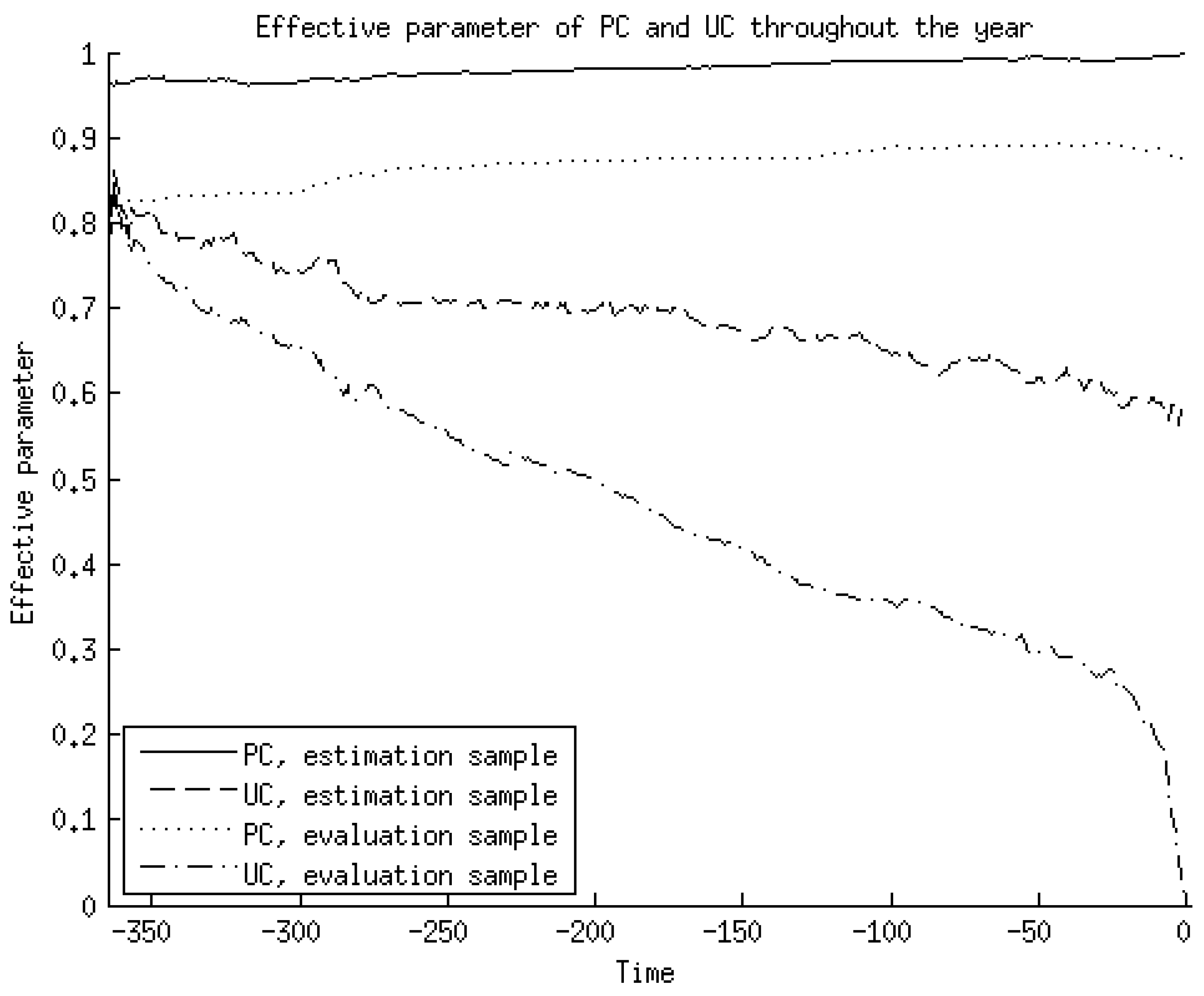
Several results from the table are interesting. First, the estimated parameters for just the predictable and the unpredictable component in the estimation sample seem to suggest that they need to be made more important than in the actual forecast (which is similar to the situation where both parameters are 1), but in actuality this is countered by the cross terms with the number of forecasts and the time until announcement, which are both strictly positive and have an associated negative parameter estimate. In fact, Figure 2 shows the effective parameters for both components throughout the year, both in the estimation and in the evaluation sample, and this figure demonstrates that the optimal contribution is always below 1 for both components. For the predictable component, the contribution is relatively stable throughout the year, while for the unpredictable component the contribution is highest in the beginning of the year.

Another result from Table 9 is that the predictable component parameters are all estimated more accurately than their unpredictable component counterparts, and the estimation results are more accurate in the estimation sample than in the evaluation sample.

Thus, this shows that the optimal contribution of the unpredictable component might be less than 1, in other words, less than what the analyst actually do. However, that does not mean that the unpredictable component does not contribute at all.

Table 10. A summary of results on the comparison between the regressions: of (1) $Actual=\alpha +\beta PC$, the actual earnings on only predictable component variables; and (2) $Actual=\alpha +\beta PCV+\gamma UC$, the actual earnings on both the predictable and unpredictable component variables. We performed these regressions for each firm separately (of the 316 firms) but pooled the results of all 18,338 forecasters. The total number of observations in the regressions across all firms is 146,319 in the estimation sample and 126,651 in the evaluation sample. The F-Statistic is based on the test for the joint significance of $\gamma$, the parameters of the unpredictable component variables, and the results for the associated P-value are shown in the column labeled P-value. The summarized results for the $R^2$ values for both the restricted and the unrestricted model are also shown.

	Estimation Sample				Evaluation Sample
	F-Statistic	P-Value	${\mathit{R}}^2$ without UC	${\mathit{R}}^2$ with UC	F-Statistic	P-Value	${\mathit{R}}^2$ without UC	${\mathit{R}}^2$ with UC
Average	33.776	0.015	0.868	0.893	29.292	0.039	0.817	0.850
Median	21.554	0.000	0.918	0.935	20.794	0.000	0.878	0.901
Standard Deviation	44.568	0.103	0.155	0.129	30.484	0.164	0.180	0.155
5% percentile	3.066	0.000	0.554	0.610	1.442	0.000	0.422	0.508
95% percentile	101.095	0.032	0.997	0.997	85.891	0.233	0.988	0.993
Significant at 5% level	96.2%				91.8%

shows results on the F-test for the joint significance of the four parameter estimates related to the unpredictable component. In both sample periods, the median F-statistic is larger than 20, and the F-test rejects no significant effect at all in more than 90% of the cases. There are clear signs that the unpredictable component does add information.

Now that we know that the unpredictable component does contribute, we can take a look at how much it contributes. Table 10 also shows the $R^2$ both when just using the predictable component variables and when also including the unpredictable component variables, for both sample periods. The increase in median $R^2$ is about 2–3%, which is not much, while the median $R^2$ using just the predictable variables is already around 90% so there is not much left to be explained.

Finally, we look at the comparison of the accuracy of this optimal forecast to the analyst forecast and model forecast, as shown in

Table 11. A summary of results on the median ratios between two squared errors. Used are combinations of the following: $F{E}^2$, the squared analyst forecast error; $PC{E}^2$, the squared error of using the predictable component as forecast; and $O{E}^2$, the squared error of the optimal combination of the predictable component and unpredictable component variables. We calculated these median ratios for each firm separately (of the 316 firms) but pooled the ratios of all 18,338 forecasters. The total number of observations across all firms is 146,319 in the estimation sample and 126,651 in the evaluation sample. We calculated some ratios in the evaluation sample twice: once with the weights (used in the construction of the optimal forecast) as estimated in the estimation sample, and once using weights based on the evaluation sample itself.

	Estimation Sample with Estimation Sample Weights			Evaluation Sample with Estimation Sample Weights			Evaluation Sample with Evaluation Sample Weights
	${\displaystyle \frac{{\mathit{FE}}^{\mathbf{2}}}{{\mathit{PCE}}^{\mathbf{2}}}}$	${\displaystyle \frac{{\mathit{OE}}^{\mathbf{2}}}{{\mathit{PCE}}^{\mathbf{2}}}}$	${\displaystyle \frac{{\mathit{OE}}^{\mathbf{2}}}{{\mathit{FE}}^{\mathbf{2}}}}$	${\displaystyle \frac{{\mathit{FE}}^{\mathbf{2}}}{{\mathit{PCE}}^{\mathbf{2}}}}$	${\displaystyle \frac{{\mathit{OE}}^{\mathbf{2}}}{{\mathit{PCE}}^{\mathbf{2}}}}$	${\displaystyle \frac{{\mathit{OE}}^{\mathbf{2}}}{{\mathit{FE}}^{\mathbf{2}}}}$	${\displaystyle \frac{{\mathit{OE}}^{\mathbf{2}}}{{\mathit{PCE}}^{\mathbf{2}}}}$	${\displaystyle \frac{{\mathit{OE}}^{\mathbf{2}}}{{\mathit{FE}}^{\mathbf{2}}}}$
Average	0.609	0.669	1.499	0.638	2.878	7.463	0.570	1.123
Median	0.655	0.532	0.877	0.631	1.107	2.165	0.311	0.591
Standard Deviation	0.304	1.206	4.425	0.571	5.703	18.399	3.097	5.330
5% percentile	0.071	0.059	0.279	0.061	0.142	0.642	0.031	0.164
95% percentile	1.031	1.371	3.437	1.207	10.102	33.621	0.943	1.757

. What can be seen is that the ratios that include the error of the optimal forecast are smaller than 1 for the samples for which the optimal relation has been determined (so when using estimation sample parameters for the estimation sample data, or evaluation sample parameters for the evaluation sample data). On the other hand, when we reuse the estimation sample parameters for the evaluation sample data, the ratio is larger than 1 compared to both the model forecast and the analyst forecast, indicating that the optimal relation is not stable over time and needs to be re-estimated regularly.

5.2. Comparison Across Forecasters

In this subsection, we aspire to find estimation sample properties of forecasters that are linked with a superior performance or a more informative unpredictable component in the evaluation sample.

5.2.1. Is It Possible to Select Forecasters Who Can Be Predicted to Outperform the Model?

First, we look at the performance of individual forecasters. A first idea might be to use again the median ratio of squared analyst forecast error to squared model forecast error as measure. This leads to a low number of forecasts on which each individual median ratio is based. In fact, it occasionally happens that the median ratio is dominated by a few observations for which either of the squared errors is almost zero. We instead want to have a more confined measure that results in a smaller interval of numbers, but that still maintains the property that a lower number means a better performance. For this, we use the balanced relative difference: $BRD(A,M)={\displaystyle \frac{AF{E}^2-MF{E}^2}{AF{E}^2+MF{E}^2}}$.

Table 12. The results for the regressions to predict better analysts in the evaluation sample using variables in the evaluation sample. This is based on 1835 forecasters (since we only include forecasters with a minimum of 10 observations in both sample periods) with a total of 52,236 forecasts in the estimation sample and 36,403 forecasts in the evaluation sample. We put the data across all firms in one regression. We used two interpretations for what a better analyst is: an analyst that has a smaller forecast error compared to the predicted component (“better performing”) and an analyst whose associated optimally constructed forecasts have smaller forecast errors compared to the predicted component error (“having more information”). These might overlap if the forecasters with more information also used them well (so if the optimal forecast is similar to the analyst forecast), but there could also be forecasters that do not use their information well, which is why we separate these measures. In these regressions we used the balanced relative difference: $BRD(x,y)=\frac{x-y}{x+y}$ with x and y being combinations of A (for the analyst forecast error, $F{E}^2$), P (for the predictable component error, $PC{E}^2$), O (for the optimal forecast error, $O{E}^2$) and U (for the squared unpredictable component, $U{C}^2$). As performance variable, we used $BRD(A,P)$, while we used $BRD(O,P)$ as information variable. The variables to be explained were measured in the evaluation sample, while the regressors were measured in the estimation sample. Standard errors are shown in parentheses. Short conclusion: (1) Better performing forecasters (low value of $BRD(A,P)$) can be predicted by looking at historically better performing forecasters and at forecasters that have relatively small unpredictable components (compared to $P{C}^2$); and (2) forecasters that have more usable information (low value of $BRD(O,P)$) can be predicted by looking at forecasters that historically have more information and forecasters that performed better.

	Variable to Explain
	$\mathit{BRD}(\mathit{A},\mathit{P})$		$\mathit{BRD}(\mathit{O},\mathit{P})$
intercept	−0.174	(0.020)	−0.003	(0.022)
$\frac{U{C}^2}{P{C}^2}$	1.152	(0.398)	0.244	(0.440)
BRD(U,P)	−0.098	(0.029)	−0.148	(0.032)
BRD(A,P)	0.407	(0.035)	0.302	(0.038)
BRD(O,P)	0.042	(0.026)	0.266	(0.029)

depicts the regression of the balanced relative difference between the analyst and model forecasts in the evaluation sample on an intercept, the ratio of the squared unpredictable component to the squared predictable component in the estimation sample and three balanced relative differences in the estimation sample: the $BRD(A,M)$ itself, but also $BRD(U,M)={\displaystyle \frac{U{C}^2-MF{E}^2}{U{C}^2+MF{E}^2}}$ and $BRD(O,M)={\displaystyle \frac{OF{E}^2-MF{E}^2}{OF{E}^2+MF{E}^2}}$. Three variables show significant results: first, $BRD(A,M)$ in the evaluation sample is significantly related to its previous value in the estimation sample, and, second, it is related to the previous value of the relative size of the unpredictable component to the predictable component and to the previous value of BRD(U,M). The results show that the forecasters that will predict best in the evaluation sample are those that have predicted best in the estimation sample, that have a small unpredictable component relative to the predictable component and that have a small unpredictable component relative to the error of the predictable component. Of these, the autoregressive type variable has the result that has the most statistical significance.

We can use the above regression to produce forecasts of the median balanced relative difference of each forecaster, and then compare the actual errors of the half that has the best performance prediction to the half that is predicted to perform worst. The ratio of the median squared error of the best 50% to the median squared error of the worst 50% is 0.600. In addition, the predicted probabilities of having a negative balanced relative difference (in other words: the probabilities of outperforming the model) are, on average, 80.8% and 61.9% for the best and worst half, respectively. This shows that it is possible to select a subset of all forecasters that will perform better in future that the entire set does.

5.2.2. Is It Possible to Select Forecasters Who Can Be Predicted to Have More Information in Their Unpredictable Component?

Next, we used a similar approach to investigate whether it is possible to select forecasters that have more useful information in their unpredictable component, in other words, for which the optimal forecast performs best. For this, we used again a balanced relative difference, for the same reasons as above. We again used a regression and we reused the regressors. The variable to be explained in this case was $BRD(O,M)$ in the evaluation sample. The results are also shown in Table 12.

Similar to the previous regression, again the autoregressive type variable is statistically most significant. The other two significant regressors are the other two balanced relative differences: $BRD(U,M)$ and $BRD(A,M)$. The forecasters with the most useful information (low $BRD(O,M)$) in the evaluation sample are those with the most useful information in the estimation sample that are most accurate in the estimation sample and, surprisingly, that have a large unpredictable component compared to the model error. We can again do as before, and compare the actual optimal forecast errors of two groups that are predicted to have the most and the least information. The relative median squared optimal forecast error is 0.566. It is possible to select a subset of the forecasters that contains those that have more informative unpredictable components.

5.2.3. Are the Informative Forecasters and the Performant Forecasters the Same?

One might wonder whether there is a significant overlap between the informative and the best-performant forecasters. To investigate this, we calculated the hit rate: the percentage of cases in which a forecaster is categorized in the same group for both measures. This hit rate is 85.4%, showing that there is definitely a pattern that the better forecasters also tend to have more information in their unpredictable components.

5.3. Comparison within Forecasters

In this subsection, we look at individual forecasts and compare their properties to other forecasts by the same forecaster. For example, the same large unpredictable component might be much more surprising if produced by someone who always has small unpredictable components than if produced by someone else who tends to produce large unpredictable components regularly. In the former case, this might indicate that this individual forecast is based on unique and important information, but it might also mean that the forecaster just has an off-day. Which of those two is true in different situations is what we investigate in this section.

First, we restricted ourselves to just the evaluation sample. The situation of comparing forecasts to other forecasts by the same forecasters meant that we often had only a few observations to compare against, and this limited us in what we can do. We did the following: we calculated for just the forecasts of one forecaster the correlation of the size of the unpredictable component with balanced relative difference variables: $BRD(A,M)$, $BRD(O,M)$ and $BRD(O,A)$, of which the latter is defined as $BRD(O,A)={\displaystyle \frac{OF{E}^2-AF{E}^2}{OF{E}^2+AF{E}^2}}$. As measures for the size of the unpredictable component we used both $\left|UC\right|$ and $U{C}^2$. Aggregate results across all forecasters are shown in

Table 13. A summary of results on the correlation between three balanced relative difference variables and two unpredictable component variables, calculated per individual forecaster. This is based on 4541 forecasters, with 90,190 forecasts in the estimation sample and 28,000 in the evaluation sample. We calculated the correlation of the $UC$-variables with three balanced relative difference variables, with the definition $BRD(x,y)=\frac{x-y}{x+y}$ with x and y being combinations of A (for the analyst forecast error, $F{E}^2$), P (for the predictable component error, $PC{E}^2$) and O (for the optimal forecast error, $O{E}^2$).

		Correlation with $\left|\mathit{UC}\right|$			Correlation with ${\mathit{UC}}^2$
		$\mathit{BRD}(\mathit{A},\mathit{P})$	$\mathit{BRD}(\mathit{O},\mathit{P})$	$\mathit{BRD}(\mathit{O},\mathit{A})$	$\mathit{BRD}(\mathit{A},\mathit{P})$	$\mathit{BRD}(\mathit{O},\mathit{P})$	$\mathit{BRD}(\mathit{O},\mathit{A})$
Estimation sample	Average	−0.096	−0.185	−0.116	−0.069	−0.166	−0.121
	Median	−0.125	−0.214	−0.133	−0.124	−0.210	−0.146
	Standard Deviation	0.322	0.279	0.273	0.335	0.278	0.272
	5% percentile	−0.582	−0.598	−0.535	−0.559	−0.556	−0.526
	95% percentile	0.454	0.324	0.359	0.506	0.354	0.358
Evaluation sample	Average	−0.146	−0.122	0.033	−0.125	−0.105	0.030
	Median	−0.173	−0.129	0.049	−0.177	−0.116	0.046
	Standard Deviation	0.477	0.490	0.472	0.481	0.487	0.468
	5% percentile	−0.953	−0.967	−0.877	−0.954	−0.963	−0.863
	95% percentile	0.790	0.852	0.909	0.816	0.835	0.892

.

Table 13 shows, after summarizing, only negative correlations are found, which have varying interpretations. The negative correlations between the size variables of UC and $BRD(A,M)$ shows that large unpredictable components for that particular forecaster are associated with a better performance compared to the model which has no unpredictable component. Similarly, the negative correlations with $BRD(O,M)$ show that large unpredictable components are associated with more information in that unpredictable component. Finally, the negative correlations with $BRD(O,A)$ show that large unpredictable components are associated with a better optimal forecast than the actual analyst forecast, and thus with less optimal use of the unpredictable component by the analyst.

Table 13 also extends the discussion to the situation in the evaluation sample. In this case, not all correlations are again negative. The ones that are (the correlations with $BRD(A,M)$ and $BRD(O,M))$ result in the same conclusion as before: large unpredictable components are associated with a better performance and more information than smaller unpredictable components produced by the same forecaster. The positive correlation of $BRD(O,A)$ with the size of the unpredictable component indicates that, in this case, on aggregate, large unpredictable components tend to coincide with less room to optimize the use of the unpredictable component compared to the analyst forecast. This difference in result compared to the estimation sample might be due to a structural change over time in how forecaster behave, but a more plausible explanation might be that the parameter estimates that are used in the construction of the optimal forecast are not stable over time, which is what we have found in Section 5.1.3.

6. Conclusions

• Earnings forecasts are an important factor in the decision making process of investors. In this paper we have shown that earnings forecasts can be predicted, which allows investors to already incorporate the predictable part in their investment decision. Furthermore, we also show that the unpredictable part of an earnings forecast can be used. One way to use it, is to improve the forecast based on just the predictable part. This is especially beneficial in the beginning of the year. Another use of the predictable and unpredictable components concerns the selection of earnings forecasters, which can be relevant if an investor wants to ignore the forecasters with a poor track record. We have shown that there is persistence in the performance of forecasters compared to the predictable component, that is, earnings forecasters who perform better in our estimation sample, also perform better, on average, in the evaluation sample. Similarly, the information in the unpredictable component, that can be used to improve the optimal forecast, is also persistent, that is, earnings forecasters whose unpredictable components are more useful in the estimation sample also have this property in the evaluation sample.
• In general, large unpredictable components seem to be a bad sign, as they are associated with large relative forecast errors. This is not the case if the earnings forecaster normally produces small unpredictable components. In that case, a large unpredictable component is a sign of both good performance and more useful information in this unpredictable component.

References

- Bolliger, Guido. 2004. The characteristics of individual analysts’ forecasts in Europe. Journal of Banking & Finance 28: 2283–309. [Google Scholar] [CrossRef]
- Brown, Lawrence D. 1993. Earnings forecasting research: its implications for capital markets research. International Journal of Forecasting 9: 295–320. [Google Scholar] [CrossRef]
- Brown, Lawrence D., and Artur Hugon. 2009. Team earnings forecasting. Review of Accounting Studies 14: 587–607. [Google Scholar] [CrossRef]
- Clement, Michael B., Jeffrey Hales, and Yanfeng Xue. 2011. Understanding analysts’ use of stock returns and other analysts’ revisions when forecasting earnings. Journal of Accounting and Economics 51: 279–99. [Google Scholar] [CrossRef]
- Clement, Michael B., and Senyo Y. Tse. 2005. Financial analyst characteristics and herding behavior in forecasting. The Journal of Finance 60: 307–41. [Google Scholar] [CrossRef]
- Cooper, Rick A., Theodore E. Day, and Craig M. Lewis. 2001. Following the leader: A study of individual analysts’ earnings forecasts. Journal of Financial Economics 61: 383–416. [Google Scholar] [CrossRef]
- Jegadeesh, Narasimhan, and Kim Woojin. 2010. Do analysts herd? An analysis of recommendations and market reactions. Review of Financial Studies 23: 901–37. [Google Scholar] [CrossRef]
- Kim, Yongtae, Gerald J. Lobo, and Minsup Song. 2011. Analyst characteristics, timing of forecast revisions, and analyst forecasting ability. Journal of Banking & Finance 35: 2158–68. [Google Scholar]
- Landsman, Wayne R., Edward L. Maydew, and Jacob R. Thornock. 2012. The information content of annual earnings announcements and mandatory adoption of IFRS. Journal of Accounting and Economics 53: 34–54. [Google Scholar] [CrossRef]
- Ramnath, Sundaresh, Steve Rock, and Philip Shane. 2008. The financial analyst forecasting literature: A taxonomy with suggestions for further research. International Journal of Forecasting 24: 34–75. [Google Scholar] [CrossRef]
- Schipper, Katherine. 1991. Analysts ’ forecasts. Accounting Horizons 5: 105–21. [Google Scholar]
- Sheng, Xuguang, and Maya Thevenot. 2012. A new measure of earnings forecast uncertainty. Journal of Accounting and Economics 53: 21–33. [Google Scholar] [CrossRef]
- Stickel, Scott E. 1990. Predicting Individual Analyst Earnings Forecasts. Journal of Accounting Research 53: 409–17. [Google Scholar] [CrossRef]