Greenhouse Emissions and Productivity Growth


1
Department of Economics, University of Crete, Rethymno 74100, Greece
2
Department of Economics, University of Cyprus, P.O. Box 20537, Nicosia 1678, Cyprus
3
Department of Economics and Finance, University of Guelph, Guelph, ON N1G 2W1, Canada
*
Author to whom correspondence should be addressed.
J. Risk Financial Manag. 2018, 11(3), 38; https://doi.org/10.3390/jrfm11030038
Submission received: 4 June 2018
/
Revised: 25 June 2018
/
Accepted: 3 July 2018
/
Published: 9 July 2018
(This article belongs to the Special Issue Nonparametric Econometric Methods and Application)
Abstract
:In this paper, we examine the effect of emissions, as measured by carbon dioxide (CO), on economic growth among a set of OECD countries during the period 1981–1998. We examine the relationship between total factor productivity (TFP) growth and emissions using a semiparametric smooth coefficient model that allow us to directly estimate the output elasticity of emissions. The results indicate that there exists a monotonically-increasing relationship between emissions and TFP growth. The output elasticity of CO emissions is small with an average sample value of 0.07. In addition, we find an average contribution of CO emissions to productivity growth of about 0.063 percent for the period 1981–1998.
1. Introduction
The natural environment and natural resources unambiguously constitute important factors of the growth process, the shortage of which may impose a limit to growth. This limit to growth may arise either from the finite amounts of certain natural resources such as raw materials or by nature’s limited ability to absorb human waste. The emphasis of the theoretical work in this area has concentrated on building growth models to study how economic policy and technological change may overcome the limits to growth imposed by the extensive use of the environment and still generate a positive long-run growth rate’ see Bovenberg and Smulder (1995), Pittel (2002) and an extensive review of the literature by Brock and Taylor (2005).
Recently, more attention has been given to the growth effects of the deterioration in the quality of the environment due to increased accumulation of emissions. Emissions, which are usually modelled as a side product of the production process (see Anderson (1987)), may affect growth through two channels. If the natural environment is considered to be an input into the production function, then emissions represent the use of environmental capital, implying a positive effect of emissions on growth. If environmental quality enters the production function as an input, then emissions exert negative effects on growth by lowering the quality of the natural environment. In both cases, any abatement efforts by society reduce the available resources for production and may harm growth.
The empirical literature on the growth-emissions debate has mainly focused on investigating the famous environmental Kuznets curve (EKC). This voluminous literature studies the empirical relationship between real per capita income and polluting emissions per unit of output; see Schmalense et al. (1998), List et al. (2003) and Azomahou et al. (2006) for some recent studies that use flexible econometric methods to study this relationship. The main result of this literature is that polluting emissions’ intensity initially rises with per capita income (at the early stages of economic development), but eventually falls as per capita income rises beyond some threshold level, at least for the case of developed economies; see Selten and Song (1994), Grossman and Krueger (1995), List and Gallet (1999) and Stern and Common (2001), among others. However, there is evidence that this relationship may not be robust for a number of emission pollutants; see Harbaugh et al. (2002) and List et al. (2003).
The evidence gathered so far is rather mixed for carbon dioxide (CO) emissions. Making use of panel data, Holtz-Eakin and Selden (1995) and Heil and Selden (2001) employed parametric models with pooled data and obtained a U-shaped EKC for CO per capita emissions. The works in Harbaugh et al. (2002), Bertinelli and Strobl (2005) and Azomahou et al. (2006) estimated non- or semi-parametric pooled regressions and nonlinear increasing shapes. Univariate approaches inspired from the income convergence literature have also been employed to explore the convergence of CO per capita emissions between countries and regions. The works in List et al. (2003), Barassi et al. (2008) and Westerlund and Basher (2008) used unit root tests to investigate stochastic convergence for different sets of countries. The results are not conclusive, but the bulk of the evidence points towards convergence. The work in Taylor and Brock (2004) estimated growth regressions for per capita CO emissions based on their Green–Solow model. The model is tested for OECD countries over the period 1960–1998, and the results suggest that most of the explanatory power comes from the initial level of CO emissions.
In terms of econometric methodology, nonparametric estimation has recently gained popularity in this literature. Among the papers that use nonparametric estimation techniques is that of Harbaugh et al. (2002), where they use a nonparametric pooled regression to examine the relationship between a CO environmental efficiency index and GDP per capita for a panel of countries. Their results indicate a U-shaped relationship followed by an inverted U relationship. The work in Bertinelli and Strobl (2005) employed a partially linear model in a cross-country context and found that a linear relationship between per capita income and SO and CO emissions cannot be rejected. The work in Azomahou et al. (2006) examined the relationship between CO emissions per capita and GDP per capita using a pooled country-fixed effects nonparametric regression, and their results indicated a monotonically-increasing relationship. The work in Bertinelli et al. (2012) investigated the CO emissions per capita-GDP per capita relationship by applying a kernel regression estimator to a panel of countries. They found that for some developed countries, the relationship between output and pollution after 1960 has been heterogeneous (for some rising, for some falling and for others flat). For almost all the developing countries in their sample, they found that the relationship was always upward sloping.
In Murdoch et al. (1997), Ansuategi (2003), Maddison (2006, 2007), another dimension was added to the empirical EKC literature, that of pollution spillovers between a set of EU countries (the dataset of Maddison (2006) is for a set of 135 countries). The empirical papers that account for transboundary pollution examine the implications of strategic interaction between countries, if any. The work in Murdoch et al. (1997) accounted for the spatial dispersion of sulphur and NOx emissions when empirically investigating the emissions reductions required by the Helsinki protocol in 25 European countries. They found that the demand for emissions reduction was higher the higher the deposition from neighbouring countries. Their model worked well for sulphur, but their results were less satisfying for NOx. The work in Ansuategi (2003) examined whether accounting for transboundary pollution affects the emissions-income relationship. He categorized countries into four groups according to their emissions and the amount of pollution they receive from other countries and estimated EKCs for each group. He found different results for different groups. The work in Helland and Whitford (2003) found that emissions releases are higher where it is likely that emissions cross state borders. On the contrary, Rupasingha et al. (2004) when examining the EKC hypothesis using U.S. county data for toxic releases, it was concluded that the EKC relationship they found was unaffected when they accounted for spatial dependence. U.S. data were also used in a study on water pollution by Sigman (2005); she used state-level data for water quality in state rivers and found evidence that states free ride. Finally, Maddison (2007) found that the quantity of transboundary imports of sulphur was statistically insignificant. However, he found that countries follow the environmental quality (per capita emissions) of their neighbours (see Maddison (2006, 2007)).
Less attention, however, has been given to the empirical investigation of the role of emissions in the production process and of the effects of emissions on economic growth. Recent studies by Tzouvelekas et al. (2006) and Vouvaki and Xepapadeas (2008) also tried to estimate the contribution of CO emissions to the growth of real per capita output. Our work differs from theirs in that we employ a technique that allows us to estimate a general production function without imposing any restrictions on its functional form. Following a different line of research, Chimeli and Braden (2005) tried to derive a link between total factor productivity (TFP) and the environmental Kuznets curve. They derived a U-shaped response of environmental quality to variations in TFP.
Polluting emissions were modelled either as an input (see, e.g., Baumol and Oates (1988)) or as an (another) output of the production process; see Fare et al. (2001). Modelling polluting emissions as an output captures the idea that good output cannot be produced unless polluting emissions (bad output) are also produced; see Fare et al. (1993), Ball et al. (1994) and Fernandez et al. (2005). In this context, emissions are a by-product of the production of goods. Those who model polluting emissions as an input argue that trying to reduce them involves diverting some of the traditional inputs into the abatement effort, something that results in fewer inputs available in the production of goods. In other words, it is argued that by reducing emissions, output is reduced, and in this sense, emissions can be treated as an input to production; see Laffont (1988), Cropper and Oates (1992), Koo (1998) and Reinhar et al. (1999). Another argument in favour of the use of polluting emissions as an input is that the latter represent the extractive use of the natural environment. That is, emissions are treated as a proxy for the use of environmental resources; see Bovenberg and Smulder (1995), Brock and Taylor (2005).
However, a number of authors argue that some of these approaches are inconsistent with the materials’ balance condition, a fundamental imperative of physical science, as well as common sense; see Murty and Russell (2002) and Murty et al. (2011). The materials’ balance approach was first introduced by Ayres and Kneese (1969), and it was only recently that it has gained attention in the modelling of emissions or production residuals in the production process; see Murty and Russell (2002), Murty et al. (2011), Pethig (2003), Pethig (2006), Førsund (2009) and Lauwers (2009). The materials’ balance condition implies that the generation of residuals inevitably arises in the process of consumption and production. The work in Murty and Russell (2002) accounted for this condition by defining a residual generating mechanism that relates the generation of production residuals to the use of polluting inputs. These polluting inputs (or material inputs as defined by others like Pethig (2003, 2006) are used in the production of the output, but are also responsible for the generation of a by-product; polluting emissions. Therefore, the link between output and polluting emissions comes through the use of the polluting generating inputs.
Although the literature on the relationship between pollution and economic growth is extensive, it ignores the role of emissions in the production process. In this paper, we investigate the empirical relationship between emissions and productivity growth using nonparametric econometric methods to uncover possible nonlinearities in the data. Proper modelling of emissions must take into account the materials’ balance condition, which further results in the intuitively desirable positive correlation between the production residuals and output. To this end, this study models the relationship between output and emissions in a manner that is consistent with the residual generation mechanism. In particular, we examine the effect of CO emissions, on economic growth among the advanced industrialized countries1. We construct a total factor productivity (TFP) index of the standard inputs, capital and labour, using the methodology that was adopted in Mamuneas et al. (2006). We then examine the relationship between TFP growth and CO emissions using a semiparametric smooth coefficient model that allows us to directly estimate the elasticity of pollution. The data covers the period from 1981–1998, for a range of OECD countries, and the results indicate that there exists a nonlinear monotonically increasing relationship between polluting emissions and economic growth as captured by TFP. This is consistent with the materials’ balance condition, which further results in the intuitively desirable positive correlation between the production residuals and output.
The paper is organized as follows. In the next section, we present the model specification and the data description. We proceed to discuss the empirical findings, and in the last section, we offer concluding remarks. In the Appendix, we present details about the econometric methodology of the smooth coefficient semiparametric model that we use and a test of linearity that we perform.
2. Methodology and Data Sources
2.1. Specification
Consider a general production function at time t as:
where Y is the total output, X is a vector of traditional inputs like physical capital K and labour inputs L, E is the energy input and t is a technology index measured by time trend. Based on the materials’ balance approach, it is assumed that emissions are generated by the usage of energy, and it is a by-product of the production process. The emissions function is defined by:
where P is the emissions variable, which is related to energy usage though the function This function is assumed to be an increasing monotonic function as it is specified by the laws of thermodynamics, that is . Inverting Equation (2), we have:
and substituting (3) in (1), we establish the link between output production and emissions; see Murty and Russell (2002) and Murty et al. (2011),
To determine the effect of emissions in the production process, we follow an approach based on Mamuneas et al. (2006), who analysed the effect of human capital on TFP growth. Total differentiation of (1) with respect to time and division by Y yields:
where (^) denotes a growth rate, is the exogenous rate of technological change and denotes output elasticity. Total differentiation of (3) with respect to time and division by E yields in growth form:
where is the energy elasticity with respect to emissions, and it is expected to be positive from the laws of thermodynamics.
Substituting Equation (5) in (4) and subtracting from both sides of Equation (4), the contribution of traditional inputs to the output growth, we get:
Note that the left-hand side of Equation (3) is directly observed from the data, if we assume a perfectly competitive environment. The output elasticities of labour and physical capital are equal to the observed output shares of labour, , and physical capital, Therefore, we can define a TFP index based on the observable data, which discretely approximates the left-hand side of Equation (6). This index allows for the contribution of each input to differ across country and time and to be dictated by the data. We define the Tornqvist index of TFP growth for country i in year t as follows:
where are the weighted average income shares of labour and physical capital and . This measure of TFP contains the components of output growth that cannot be explained by the growth of the inputs ( in Equation (6).
On the right-hand side of (6), the unobserved contribution of emissions to output growth is assumed to be an unknown function of the level of emissions i.e., . Note that the function captures the effect of emissions on productivity growth, and it can be only positive since it captures the combined effects of energy and emissions. Hence, putting all together, in a discrete form, Equation (6) can be written as:
where Equation (8) can be estimated using semiparametric methods. It allows emissions to influence TFP growth in a nonlinear fashion. In the equation above, can be considered as a function of country- and year-specific dummy variables. Country specific dummies, , capture idiosyncratic exogenous technological change, and time specific dummies, , capture procyclical behaviour of TFP growth. The equation of interest now becomes:
If we let and where can be any other variable included in the smooth coefficient function, the model can be written more compactly as:
For proper estimation, we assume that where denotes the expectations operator.
We proceed to estimate the model of Equation (9) using a smooth varying coefficient semiparametric estimator. A smooth coefficient semiparametric model is considered to be a useful and flexible specification for studying a general regression relationship with varying coefficients. It is a special form of varying coefficient models, and it is based on polynomial regression; see Fan (1992), Fan and Zhang (1999), Li et al. (2002) and Mamuneas et al. (2006), among others. A semiparametric varying coefficient model imposes no assumption on the functional form of the coefficients, and the coefficients are allowed to vary as smooth functions of other variables. Specifically, varying coefficient models are linear in the regressors, but their coefficients are allowed to change smoothly with the value of other variables. In the Appendix, we present the mechanics of the method in more detail.
2.2. Data Sources
In order to investigate the empirical relationship between emissions and aggregate output, we collected data from the World Bank and the OECD databases covering a wide range of countries over the period 1981–1998. The countries chosen were based on the availability of pollution data, as well as physical capital and emissions data. The countries included in this analysis are: Australia, Austria, Belgium, Canada, Denmark, Finland, France, Greece, Ireland, Italy, Korea, the Netherlands, Portugal, Spain, Sweden, the U.K. and the USA.
The OECD databases provide data on GDP, employment and capital formation. All data are in millions of Euros, and the base year is 2000. Since energy is introduced as a paid input of production, which generates an unpaid by-product, emissions, the aggregate output measure has to be adjusted to include the contribution of energy. In other words, if energy is to be added on the right-hand side of the aggregate production function, then output would need to be adjusted, as well. Hence, the value of output used is a gross output measure, which consists of the value added in current prices plus the value of energy consumption. Output, is defined then by deflating the above gross output measure by the GDP deflator. Labour input, is defined as the total man-hours (total number of workers times hours worked), and the capital stock, was constructed by accumulating gross investment in constant prices, using the perpetual inventory method, with a depreciation rate of 4%. Finally, the energy input, is constructed by dividing the value of energy consumption by the GDP deflator. The consumption of energy has been obtained from the EU KLEMS Growth and Productivity Accounts database2. As a proxy for emission flow, we used CO emissions, obtained from the 2002 World Development Indicators. According to the World Bank definition, CO emissions (kilotons (kt)) are those stemming from the burning of fossil fuels and the manufacture of cement. They include contributions to the carbon dioxide produced during consumption of solid, liquid and gas fuels and gas flaring.
As a proxy for pollution flow, we used CO emissions, obtained from the 2002 World Development Indicators. According to the World Bank definition, CO (carbon dioxide) emissions (kt) are those stemming from the burning of fossil fuels and the manufacture of cement. They include contributions to the carbon dioxide produced during consumption of solid, liquid and gas fuels and gas flaring. CO is a stable gas, which is not transformed chemically in the atmosphere. However, some CO is removed from the atmosphere by a natural process that includes the effect of vegetation, soils and oceans. Moreover, human activities such as reforestation, deforestation or land management may increase or decrease the amount of CO removed from the atmosphere. This degree of atmospheric removal because of combined natural and human activities corresponds to a depreciation rate that is used to construct the total “stock” of accumulated pollution. The global natural CO removal rate for the set of countries that we examine has been estimated to be around 60 percent for the period 1980–1989 and 52 percent for the 1989–1998 period; see IPCC (2000). If one adds the human-induced changes in land use and forestry, we derive country-specific values on the basis of CO emission data provided on the website of the United Nations Framework Convention on Climate Change (UNFCCC)3. As part of their obligation, countries report to the UNFCCC their annual emissions of greenhouse gases, with data currently spanning the period 1990–2004. For all countries in our sample, emissions are provided with and without taking into account CO removal resulting from direct human-induced land use, land use change and forestry (LULUCF). The ratio of emissions with LULUCF over emissions without LULUCF gives the rate of CO removal because of human activities. The overall removal rate (depreciation rate) from both human activities and natural processes for the countries in our sample over the period that we examine is around seventy percent, which is what we use in our estimation to construct the total “stock” of accumulated pollution.
To express emissions in concentration terms, which is a more appropriate measure of pollution (see Brock and Taylor (2005)), we divide total emissions with the surface of each country so that our pollution variable, measures CO emissions in kilotons per square kilometre. This is a measure of pollution intensity, and it is closely related to pollution concentration, which is emissions measured as milligrams per cubic meter. The implication of this new pollution intensity concentration variable for our empirical specification is that the damage caused by CO emission to the environment depends on the size of the natural environment4.
3. Empirical Findings
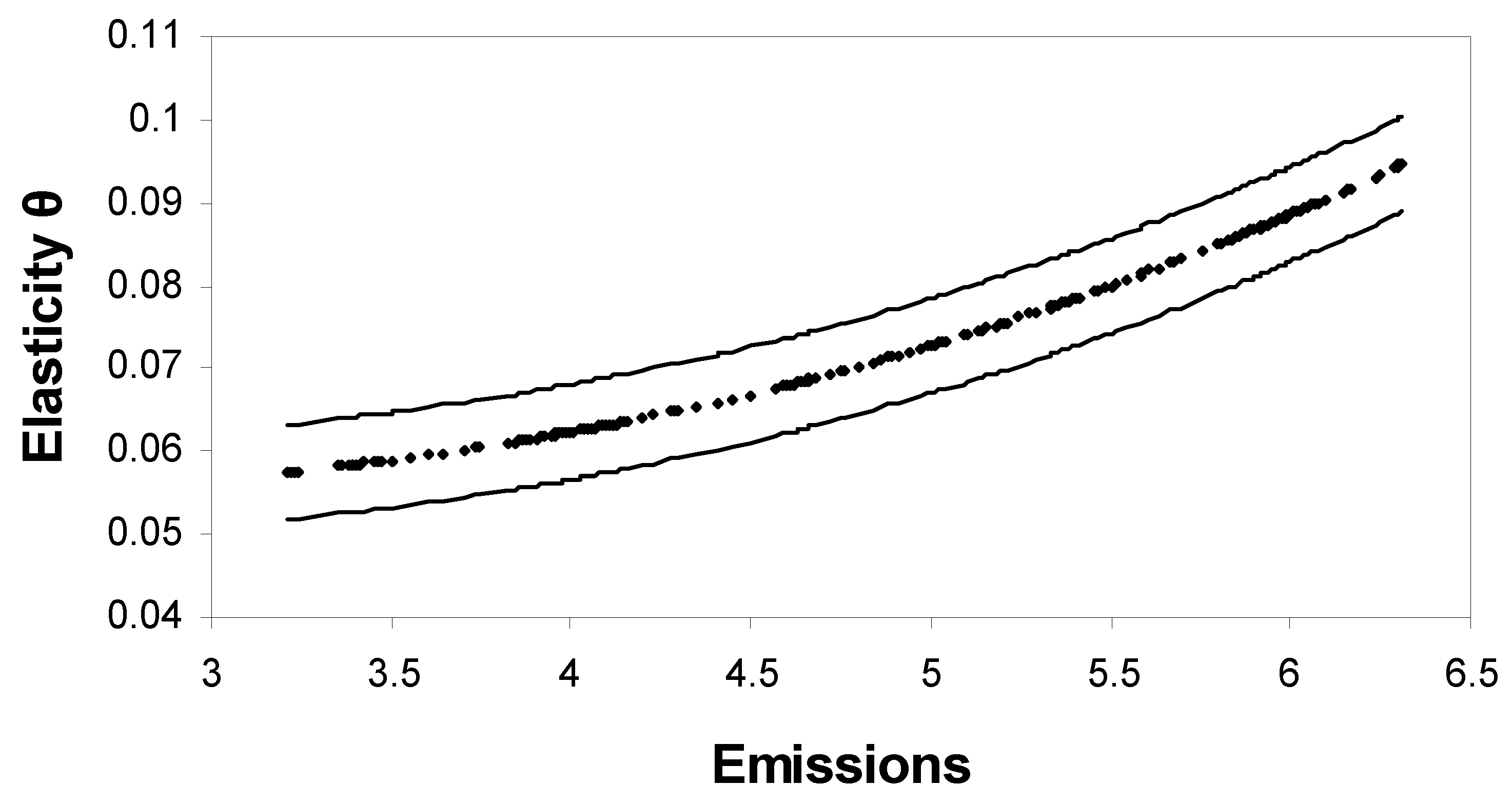
We estimate the model of Equation (9) using a smooth coefficient semiparametric estimator. In Equation (9), the variables of interest are expressed in growth terms, and they are all . Our approach is different from univariate approaches inspired by the income convergence literature that have also been employed to explore the convergence of CO per capita emissions between countries and regions using data in levels. The works in List et al. (2003), Barassi et al. (2008) and Westerlund and Basher (2008) used unit root tests to investigate stochastic convergence for different sets of countries. In our paper, we are particularly interested in the unknown coefficient function . The results are presented in Figure 1. The effect of polluting emissions on growth is positive and monotonically increasing. This result is consistent with the materials’ balance condition where the generation of emission residuals inevitably arises in the production process. Our overall finding is that the effect of pollution emissions on growth is positive and nonlinear. This implies that the productivity effect dominates any negative externality effects. It is nearly constant up to a certain level of pollution intensity, and then, it appears to accelerate at higher levels. The presence of such a threshold effect is consistent with the presence of newer pollution abatement technologies “cleaner technologies” that kick in at higher levels of pollution and are responsible for increasing productivity gains. These productivity gains might also come from a reduction of negative pollution externalities due to abatement. It is interesting to note that the above finding can be also given an EKC interpretation as it would correspond to the second half of the U relationship that has been found in the literature, and given that our dataset consists of developed countries, this is consistent with the EKC evidence. This is consistent, for instance, with the evidence found in Stern and Common (2001) for another pollutant, sulphur, for the group of developed economies similar to the ones we examine.
We proceed to test the specification of our model. First, we test that the model that generated the data in the graphs of Figure 1 is linear. In the Appendix, we present the mechanics of the linearity test that we employ. We strongly reject the null hypothesis of linearity with a p-value less than 0.001 for the test statistic that we obtained. Next, we proceed to investigate the robustness of our findings. We first check for possible endogeneity in the model by following Cai et al. (2006), who propose an Intrumental Variables (IV) methodology for smooth coefficient models based on local linear methods. We obtain fitted values of current emissions and emission growth as functions of past output and emissions as instruments, which we then use in the second stage, as suggested by Cai et al. (2006). We tried different sets of past values, but the results were fairly robust, and the shape of the graph in Figure 1 was left essentially intact, irrespective of the different instruments used5.
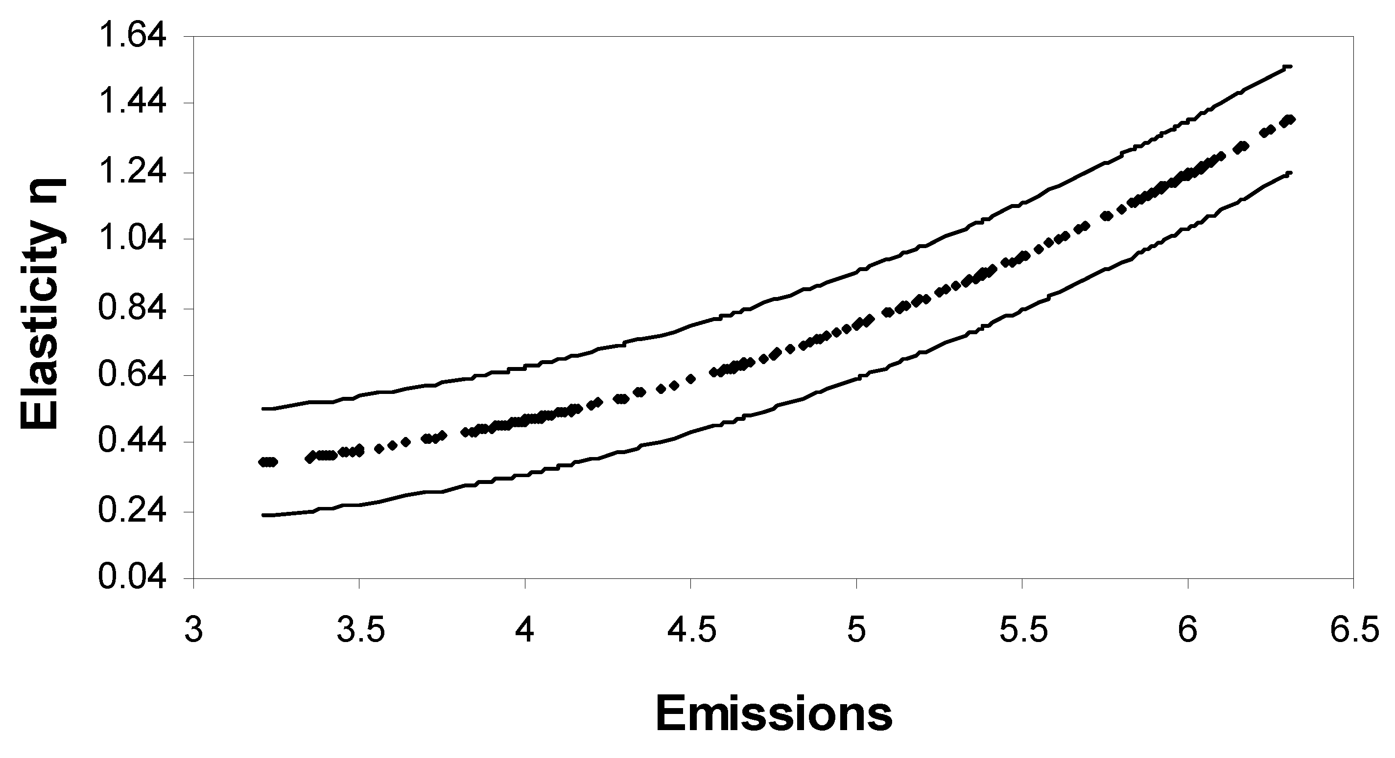
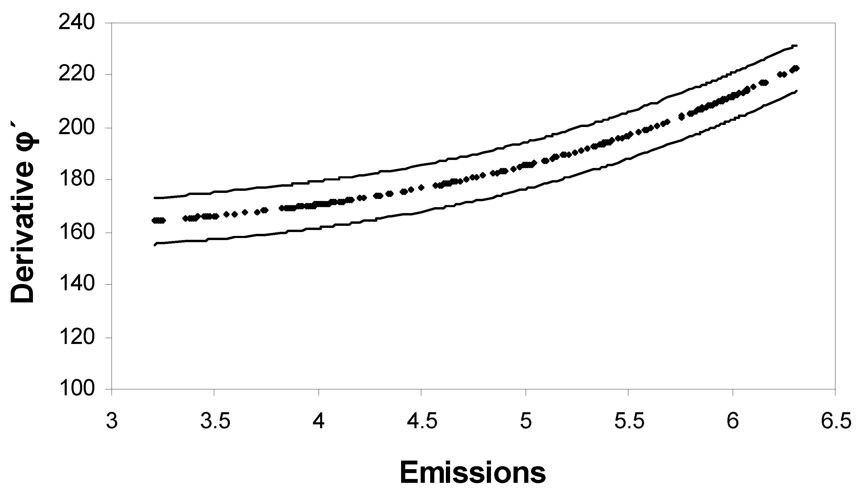
Finally, since the estimates of elasticities depends on two unknown elasticities, the elasticity of output with respect to energy, and the inverse elasticity of emissions with respect to energy, we have estimated two alternative specifications. Firstly, it is assumed that the output elasticity of energy is given by the observed energy share, and therefore, the unknown parameter to be estimated is i.e., Secondly, the inverse marginal effect of energy on emissions, is directly estimated observing that The graphs of these specifications are presented in Figure 2 and Figure 3, respectively. It is apparent that the total elasticity and the shape of the graph in Figure 1 remain unchanged irrespective of the parameter restrictions imposed.
To examine the effect per country, we have calculated the average output elasticity of emissions per country, and the results are presented in the first column of Table 1. The results indicate that the average elasticity of emission for all countries is 0.07 and significantly different from zero. This implies that a 1% increase of emissions increases on average the output by only 0.07%. In addition, it is clear from the table that the average elasticity of emissions per country varies according to the country’s emission levels. It is interesting to note that the most industrialized countries have also the highest output elasticities, like the USA, Canada and the U.K. The second column of Table 1 provides the average contribution of CO emissions growth on total factor productivity (TFP) growth. The results vary by country, depending on the output elasticity of emissions and the emissions growth rate. These results indicate that the effect of emissions on TFP growth and hence output growth is significant, but rather small for most countries of the sample For the period of consideration (1981–1998) emissions contributed positively to TFP growth in most of the countries that we consider, while they contributed negatively in some countries like Belgium, Sweden and the U.K., for example, due to the decline of their CO emissions.
4. Conclusions
In this paper, we have studied the effect of emissions, as measured by CO, on economic growth among the advanced industrialized countries. We construct a TFP growth index by subtracting from the output growth the weighted growth of physical capital and labour inputs, using the observed income shares of physical capital and labour as weights. The TFP index based on the observable data allows for the contribution of each input to differ across country and time and to be dictated by the data. We then examine the relationship between TFP growth and emissions using a semiparametric smooth coefficient model that allows us to directly estimate the elasticity of emissions.
Our results indicate that there exists a robust nonlinear relationship between CO and economic growth as captured by TFP growth. We find that the CO emissions effect varies depending on a country’s emissions level. In addition, we find a monotonically-increasing relationship between emissions and output, a result that is consistent with the materials’ balance condition. Overall, emission elasticities vary among different countries with an average elasticity (for all countries) of 0.07. Finally, we find that CO emissions contribute on average about 0.063% to productivity growth in the countries of our sample for the period 1981–1998.
Author Contributions
All authors have contributed equally.
Funding
This research was funded by Social Science and Humanities Research Council of Canada, grant number 4301.
Acknowledgments
We would like to thank Theodoros Zachariades for helpful comments. The third author would like to acknowledge financial support from Social Science and Humanities Council of Canada.
Conflicts of Interest
The authors declare no conflict of interest.
Appendix A. Econometric Estimation: A Smooth Coefficient Semiparametric Approach
A semiparametric varying coefficient model imposes no assumption on the functional form of the coefficients, and the coefficients are allowed to vary as smooth functions of other variables. Specifically, varying coefficient models are linear in the regressors, but their coefficients are allowed to change smoothly with the value of other variables. One way of estimating the coefficient functions is by using a local least squares method with a kernel weight function. A semiparametric smooth coefficient model is given by:
where denotes the dependent variable (the TFP index as discussed earlier), denotes a vector of variables of interest (in the case of Equation (6), and denotes a vector of other exogenous variables (the from Equation (5) above) and is a vector of unspecified smooth functions of ( in Equation (6)). To simplify the exposition, we ignore the partially linear nature of Equation (6), by suppressing for now the vector of the . Based on Li et al. (2002), the above semiparametric model has the advantage that it allows more flexibility in functional form than a parametric linear model or a semiparametric partially linear specification. Furthermore, the sample size required to obtain a reliable semiparametric estimation is not as large as that required for estimating a fully nonparametric model. It should be noted that when the dimension of is greater than one, this model also suffers from the “curse of dimensionality”, although to a lesser extent than a purely nonparametric model where both and enter nonparametrically. The work in Fan and Zhang (1999) suggested that the appeal of the varying coefficient model is that by allowing coefficients to depend on other variables, the modelling bias can significantly be reduced, and the curse of dimensionality can be avoided. Equation (6) above can be rewritten as:
where is a smooth but unknown function of One can estimate using a local least squares approach, where:
is a kernel function, and is the smoothing parameter for sample size The intuition behind the above local least squares estimator is straightforward. Let us assume that z is a scalar and is a uniform kernel. In this case, the expression for becomes:
In this case, is simply a least squares estimator obtained by regressing on using the observations of that their corresponding is close to z Since is a smooth function of is small when is small. The condition that is large ensures that we have sufficient observations within the interval when is close to Therefore, under the conditions that and , one can show that the local least squares regression of on provides a consistent estimate of In general, it can be shown that:
where can be consistently estimated. The estimate of can be used to construct confidence bands for We use a standard multivariate kernel density estimator with a Gaussian kernel and cross-validation to choose the bandwidth.
An interesting special case of Equation (A2) is when the from Equation (6) are taken into account. In that case, some of the coefficients in Equation (A2) are constants (independent of In that case, Equation (A2) can be rewritten as:
where is the i-th observation on a vector of additional regressors that enter the regression function linearly (in our case where W, the country specific and time dummies . The estimation of this model requires some special treatment as the partially-linear structure may allow for efficiency gains, since the linear part can be estimated at a much faster rate, namely
The partially-linear model in Equation (A3) has been studied by Zhang et al. (2002) and Ahmad et al. (2005). The work in Zhang et al. (2002) suggests a two-step procedure where the coefficients of the linear part are estimated in the first step using polynomial fitting with an initial small bandwidth using cross-validation; see Hoover et al. (1998). In other words, the approach is based on undersmoothing in the first stage. Then, these estimates are averaged to yield the final first step linear part estimates, which are then used to redefine the dependent variable and return to the environment of Equation (A1) where local smoothers can be applied as described above.
Appendix B. Linearity Test
We will present below a test statistic that was used by Li et al. (2002). In our implementation, we will use a bootstrap version of this test. Let denote the dependent variable, and let be and be vectors of exogenous variables. Consider the following linear model:
where is a smooth known function of For example, in the context of Equation (2), ignoring for the moment the presence of the we have and Similarly, Equation (A1) captures the case of the augmented version of (2) to allow for the simple interactions of the with where and
We can test the adequacy of (A1), against the semiparametric alternative (1) using the following test statistic.
where denotes the residual from parametric estimation (under It can be shown that under where is a consistent estimator of the variance of ; see Li et al. (2002). It can be shown that the test statistic is a consistent test for testing (Equation (3)) against (Equation (1)). We use a bootstrap version of the above test statistic, since bootstrapping improves the size performance of kernel-based tests for the functional form; see Zheng (1996) and Li and Wang (1998).
References
- Ahmad, Ibrahim, Sittisak Leelahanon, and Qi Li. 2005. Efficient estimation of a semiparametric partially varying linear model. Annals of Statistics 33: 258–83. [Google Scholar] [CrossRef]
- Anderson, Curt L. 1987. The production process: Inputs and wastes. Journal of Environmental Economics and Management 14: 1–12. [Google Scholar] [CrossRef]
- Ansuategi, Alberto. 2003. Economic growth and transboundary pollution in Europe: An empirical analysis. Environmental and Resource Economics 26: 305–28. [Google Scholar] [CrossRef]
- Ayres, Robert U., and Allen V. Kneese. 1969. Production, Consumption, and Externalities. American Economic Review 59: 282–97. [Google Scholar]
- Azomahou, Theophile, François Laisney, and Phu Nguyen Van. 2006. Economic development and CO2 emissions: A nonparametric panel approach. Journal of Public Economics 90: 1347–63. [Google Scholar] [CrossRef]
- Ball, V. Eldon, Ca Knox Lovell, Richard Nehring, and Agapi Somwaru. 1994. Incorporating Undesirable Outputs into Models of Production: An Application to US Agricultural. Cahiers d’Economique et Sociologie Rurales 31: 59–73. [Google Scholar]
- Barassi, Marco R., Matthew A. Cole, and Robert J. R. Elliott. 2008. Stochastic divergence or convergence of per capita carbon dioxide emissions: Re-examining the evidence. Environmental and Resource Economics 40: 121–37. [Google Scholar] [CrossRef]
- Baumol, William J., and Wallace E. Oates. 1988. The Theory of Environmental Policy, 2nd ed. Cambridge: Cambridge U. Press. [Google Scholar]
- Bertinelli, Luisito, and Eric Strobl. 2005. The Environmental Kuznets Curve semi-parametrically revisited. Economics Letters 88: 350–57. [Google Scholar] [CrossRef]
- Bertinelli, Luisito, Eric Strobl, and Benteng Zou. 2012. Sustainable economic development and the environment: Theory and evidence. Energy Economics 34: 1105–14. [Google Scholar] [CrossRef]
- Bovenberg, A. Lans, and Sjak Smulder. 1995. Environmental quality and pollution-augmenting technological change in a two-sector endogenous growth model. Journal of Public Economics 57: 369–91. [Google Scholar] [CrossRef]
- Brock, William A., and M. Scott Taylor. 821. Economic growth and the environment: A review of theory and empirics. In Handbook of Economic Growth II. Edited by Aghion Philippe and Durlauf Steven. New York: Elsevier, Chp. 28. pp. 369–1749. [Google Scholar]
- Cai, Zongwu, Mitali Das, Huaiyu Xiong, and Xizhi Wu. 2006. Functional coefficient instrumental variable models. Journal of Econometrics 133: 207–41. [Google Scholar] [CrossRef]
- Chimeli, Ariaster B., and John B. Braden. 2005. Total factor productivity and the environmental Kuznets curve. Journal of Environmental Economics and Management 49: 366–80. [Google Scholar] [CrossRef]
- Cropper, Maureen L., and Wallace E. Oates. 1992. Environmental Economics: A survey. Journal of Economic Literature 30: 675–740. [Google Scholar]
- Fan, Jianqing. 1992. Design-adaptive nonparametric regression. Journal of the American Statistical Association 87: 998–1004. [Google Scholar] [CrossRef]
- Fan, Jianqing, and Wenyang Zhang. 1999. Statistical estimation in varying-coefficient models. Annals of Statistics 27: 1491–518. [Google Scholar]
- Fare, Rolf, Shawna Grosskopf, C. A. Knox Lovell, and Suthathip Yaisawarng. 1993. Derivation of shadow prices for undesirable outputs: A distance function approach. Review of Economics and Statistics 75: 375–80. [Google Scholar] [CrossRef]
- Fare, Rolf, Shawna Grosskopf, and Carl A. Pasurka Jr. 2001. Accounting for air pollution emissions in measures of state manufacturing productivity growth. Journal of Regional Science 41: 381–409. [Google Scholar] [CrossRef]
- Fernandez, Carmen, Gary Koop, and Mark F. J. Steel. 2005. Alternative efficiency measures for multiple-output production. Journal of Econometrics 126: 411–44. [Google Scholar] [CrossRef] [Green Version]
- Førsund, Finn R. 2009. Good Modelling of Bad Outputs: Pollution and Multiple-Output Production. International Review of Environmental & Recourse Economics 3: 1–38. [Google Scholar] [Green Version]
- Grossman, Gene M., and Alan B. Krueger. 1995. Economic growth and the environment. Quarterly Journal of Economics 110: 353–77. [Google Scholar] [CrossRef]
- Harbaugh, William T., Arik Levinson, and David Molloy Wilson. 2002. Reexamining the empirical evidence for an environmental Kuznets curve. Review of Economics and Statistics 84: 541–51. [Google Scholar] [CrossRef]
- Heil, Mark T., and Thomas M. Selden. 2001. Carbon emissions and economic development: Future trajectories based on historical experience. Environment and Development Economics 6: 63–83. [Google Scholar] [CrossRef]
- Helland, Eric, and Andrew B. Whitford. 2003. Pollution incidence and political jurisdiction: Evidence from TRI. Journal of Environmental Economics and Management 46: 403–24. [Google Scholar] [CrossRef]
- Holtz-Eakin, Douglas, and Thomas M. Selden. 1995. Stocking the fires? CO2 emissions and economic growth. Journal of Public Economics 57: 85–101. [Google Scholar] [CrossRef]
- Hoover, Donald R., John A. Rice, Colin O. Wu, and Li-Ping Yang. 1998. Nonparametric Smoothing Estimates of Time-Varying Coefficient Models with Longtitudinal Data. Biometrica 85: 809–22. [Google Scholar] [CrossRef]
- IPCC. 2000. IPCC Special Report on Land Use Change and Forestry-Summary for Policymakers. Geneva: Intergovernmental Panel on Climate Change, Available online: https://www.ipcc.ch/pdf/special-reports/spm/srl-en.pdf (accessed on 5 July 2018).
- Koop, Gary. 1998. Carbon Dioxide emissions and economic growth: A structural approach. Journal of Applied Statistics 25: 489–515. [Google Scholar] [CrossRef]
- Laffont, Jean-Jacque. 1988. Fundamentals of Public Economics. Cambridge: MIT Press. [Google Scholar]
- Lauwers, Ludwig. 2009. Justifying the incorporation of the materials balance principle into frontier-based eco-efficiency models. Ecological Economics 68: 1605–14. [Google Scholar] [CrossRef]
- Li, Qi, Cliff J. Huang, Dong Li, and Tsu-Tan Fu. 2002. Semiparametric smooth coefficient models. Journal of Business Econom 20: 412–22. [Google Scholar] [CrossRef]
- Li, Qi, and Suojin Wang. 1998. A Simple Consistent Bootstrap Test for a Parametric Regression Functional Form. Journal of Econometrics 87: 145–65. [Google Scholar] [CrossRef]
- List, John A., and Craig A. Gallet. 1999. The environmental Kuznets curve: Does one size fit all? Ecological Economics 31: 409–23. [Google Scholar] [CrossRef]
- Millimet, Daniel L., John A. List, and Thanasis Stengos. 2003. The environmental Kuznets curve: Real progress or misspecified models? Review of Economics and Statistics 85: 1038–47. [Google Scholar] [CrossRef]
- Maddison, David. 2006. Environmental Kuznets Curves: A spatial econometric approach. Journal of Environmental Economics and Management 51: 218–30. [Google Scholar] [CrossRef]
- Maddison, David. 2007. Modelling sulphur in Europe: A spatial econometric approach. Oxford Economics Paper 59: 726–43. [Google Scholar] [CrossRef]
- Mamuneas, Theofanis P., Andreas Savvides, and Thanasis Stengos. 2006. Economic development and the return to human capital: A smooth coefficient semiparametric approach. Journal of Applied Econometrics 21: 111–32. [Google Scholar] [CrossRef]
- Murdoch, James C., Tod Sandler, and Keith Sargent. 1997. A tale of two collectives: Sulphur versus nitrogen oxide emission reduction in Europe. Economica 64: 281–301. [Google Scholar] [CrossRef]
- Murty, Sushama, and R. Robert Russell. 2002. On Modelling Pollution-Generating Technologies. Riversid: Department of Economics, University of Californiae. [Google Scholar]
- Murty, Sushama, R. Robert Russell, and Steven B. Levkoff. 2011. On Modelling Pollution-Generating Technologies. Discussion Paper 11/1. Exeter: Department of Economics, University of Exeter, ISSN 1473-3307. [Google Scholar]
- Pethig, Rüdiger. 2003. The ‘Materials Balance Approach’ to Pollution: Its Origin, Implications and Acceptance. Economics Discussion Paper No. 105-03. Siegen: University of Siegen. [Google Scholar]
- Pethig, Rüdiger. 2006. Nonlinear Production, Abatement, Pollution and Materials Balance Reconsidered. Journal of Environmental Economics and Management 51: 185–204. [Google Scholar] [CrossRef]
- Pittel, Karen. 2002. Sustainability and Economic Growth. Cheltenham: Edward Elgar. [Google Scholar]
- Reinhard, Stijn, C. A. Knox Lovell, and Geert Thijssen. 1999. Econometric Estimation of Technical and Environmental Efficiency: An Application to Dutch Dairy Farms. American Journal of Agricultural Economics 81: 44–60. [Google Scholar] [CrossRef]
- Rupasingha, Anil, Stephan J. Goetz, David L. Debertin, and Angelos Pagoulatos. 2004. The environmental Kuznets curve for US counties: A spatial econometric analysis with extensions. Papers in Regional Science 83: 407–24. [Google Scholar] [CrossRef]
- Schmalensee, Richard, Thomas M. Stoker, and Ruth A. Judson. 1998. World Carbon Dioxide Emissions: 1950–2050. The Review of Economics and Statistics 80: 15–27. [Google Scholar] [CrossRef]
- Selden, Thomas M., and Daqing Song. 1994. Environmental quality and development: Is there a Kuznets curve for air pollution emission? Journal of Environmental Economics and Management 27: 147–62. [Google Scholar] [CrossRef]
- Sigman, Hilary. 2005. Transboundary spillovers and decentralization of environmental policies. Journal of Environmental Economics and Management 50: 82–101. [Google Scholar] [CrossRef] [Green Version]
- Stern, David I., and Michael S. Common. 2001. Is there an Environmental Kuznets curve for sulphur? Journal of Environmental Economics and Management 41: 162–78. [Google Scholar] [CrossRef]
- Taylor, M. Scott, and William A. Brock. 2004. The Green Solow Model. NBER Working Paper 10557. Calgary, AB, Canada: University of Calgary. [Google Scholar]
- Tzouvelekas, Vangelis, Dimitra Vouvaki, and Anastasios Xepapadeas. 2006. Total Factor Productivity and the Environment: A Case for Green Growth Accounting. Crete: University of Crete. [Google Scholar]
- Vouvaki, Dimitra, and Anastasios Xepapadeas. 2008. Total Factor Productivity Growth when Factors of Production Generate Environmental Externalities. MPRA Paper 10237. Munich: University of Munich. [Google Scholar]
- Westerlund, Joakim, and Syed A. Basher. 2008. Testing the convergence in carbon dioxide emissions using a century of panel data. Environmental and Resource Economics 40: 109–20. [Google Scholar] [CrossRef] [Green Version]
- Zhang, Wenyang, Sik-Yum Lee, and Xinyuan Song. 2002. Local polynomial fitting in semivarying coefficient model. Journal of Multivariate Analysis 82: 166–88. [Google Scholar] [CrossRef]
- Zheng, John Xu. 1996. A Consistent Test of Functional Form via Nonparametric Estimation Techniques. Journal of Econometrics 75: 263–89. [Google Scholar] [CrossRef]
| 1 | Even though as mentioned above, studies that examine the EKC have used different pollutants besides CO, we concentrate on CO as it best captures the use of energy in a production function setting that underlies our TFP approach. |
| 2 | The site for the data is: www.euklems.net/eukdata.shtml. |
| 3 | |
| 4 | In the science of economic growth, it is customary to express variables in a per capita basis. However, in the environmental engineering literature, it is the concentration of pollution that is of interest. In our case, the elasticity of pollution intensity that we estimate is the same as that of pollution concentration, and as such, it is the appropriate concept to use. Another possible standardization, division by total GDP, is likely to introduce endogeneity issues. |
| 5 | However, we should note that our model is more complicated than Cai et al. (2006) as endogeneity enters both the variable in the unknown coefficient function, as well as the regressor. In this case, the asymptotic variance component will be different than theirs. However, deriving the correct asymptotic variance for a functional coefficient of this model goes beyond the scope of the present paper. |
Figure 1.
Output elasticity of emissions.

Figure 2.
Elasticity of emissions.

Figure 3.
Marginal effect of emissions.


Table 1.
Output elasticity of emissions.
| Contribution to TFP Growth Average 1981–1998 (Stand. Error) | ||
|---|---|---|
| Country | Elasticity | TFP Contribution |
| Australia | 0.0721 (0.0001) | 0.00198 (0.00012) |
| Austria | 0.0553 (0.0001) | 0.00061 (0.00012) |
| Belgium | 0.0607 (0.0001) | −0.00086 (0.00012) |
| Canada | 0.0804 (0.0001) | 0.00047 (0.00011) |
| Denmark | 0.0555 (0.0001) | −0.00051 (0.00011) |
| Finland | 0.0546 (0.0001) | −0.00018 (0.00001) |
| France | 0.0778 (0.0001) | −0.00112 (0.00025) |
| Greece | 0.0568 (0.0001) | 0.00157 (0.00014) |
| Ireland | 0.0515 (0.0001) | 0.00121 (0.00009) |
| Italy | 0.0784 (0.0001) | 0.00048 (0.00008) |
| Korea | 0.0711 (0.0001) | 0.00415 (0.00012) |
| The Netherlands | 0.0642 (0.0001) | 0.00028 (0.00005) |
| Portugal | 0.0529 (0.0001) | 0.00208 (0.00009) |
| Spain | 0.0690 (0.0001) | 0.00084 (0.00006) |
| Sweden | 0.0551 (0.0001) | −0.00116 (0.00007) |
| U.K. | 0.0849 (0.0001) | −0.00032 (0.00003) |
| USA | 0.1266 (0.0001) | 0.00116 (0.00009) |
| Average | 0.0686 (0.0001) | 0.00063 (0.00003) |
© 2018 by the authors. Licensee MDPI, Basel, Switzerland. This article is an open access article distributed under the terms and conditions of the Creative Commons Attribution (CC BY) license (http://creativecommons.org/licenses/by/4.0/).
Share and Cite
MDPI and ACS Style
Kalaitzidakis, P.; Mamuneas, T.P.; Stengos, T. Greenhouse Emissions and Productivity Growth. J. Risk Financial Manag. 2018, 11, 38. https://doi.org/10.3390/jrfm11030038
AMA Style
Kalaitzidakis P, Mamuneas TP, Stengos T. Greenhouse Emissions and Productivity Growth. Journal of Risk and Financial Management. 2018; 11(3):38. https://doi.org/10.3390/jrfm11030038
Chicago/Turabian StyleKalaitzidakis, Pantelis, Theofanis P. Mamuneas, and Thanasis Stengos. 2018. "Greenhouse Emissions and Productivity Growth" Journal of Risk and Financial Management 11, no. 3: 38. https://doi.org/10.3390/jrfm11030038