Forecasting Volatility: Evidence from the Saudi Stock Market

Abstract

The purpose of this paper is to evaluate the forecasting performance of linear and non-linear generalized autoregressive conditional heteroskedasticity (GARCH)–class models in terms of their in-sample and out-of-sample forecasting accuracy for the Tadawul All Share Index (TASI) and the Tadawul Industrial Petrochemical Industries Share Index (TIPISI) for petrochemical industries. We use the daily price data of the TASI and the TIPISI for the period of 10 September 2007 to 26 February 2015. The results suggest that the Asymmetric Power of ARCH (APARCH) model is the most accurate model in the GARCH class for forecasting the volatility of both the TASI and the TIPISI in the context of petrochemical industries, as this model outperforms the other models in model estimation and daily out-of-sample volatility forecasting of the two indices. This study is useful for the dataset examined, because the results provide a basis for traders, policy-makers, and international investors to make decisions using this model to forecast the risks associated with investing in the Saudi stock market, within certain limitations.

1. Introduction

Given that it affects consumer spending, investors’ willingness to hold risky assets, and corporations’ investment decisions, stock market volatility has a number of implications for the real economy (e.g., Fornari and Mele 2009). Understanding volatility, forecasting it accurately, and managing the exposure to risk of an investment portfolio are all crucial to making sound investment decisions (Figlewski 2004). Further, forecasting volatility is critical in many areas of finance, such as Value-at-Risk applications, option pricing, and portfolio selection (Gabriel 2012). Thus, a growing body of literature is focused on modeling and forecasting stock market risks in both developed and emerging markets (Patev and Kanaryan 2008, 2009; Carvalho et al. 2006; Kovačić 2007; Hamadu and Ibiwoye 2010; Wei et al. 2010; Gabriel 2012; Al Rahahleh 2017) to explore the extent of volatility in the current stock market environment and the impact of volatility in this context.

Recent years have seen strong interest in oil price volatility on the part of a number of researchers, who have found that it has an impact on stock market returns. For example, Basher and Sadorsky (2006) found that changes in the price of oil has an effect on stock returns in emerging markets. Mohanty et al. (2011) showed that at the country level, stock markets have significant positive exposure to oil price shocks, and that oil price changes have asymmetric effects on stock market returns at both the country and industry levels. Further, by using vector autoregression (VAR models) and co-integration tests, Hammoudeh and Aleisa (2004) found a bidirectional relationship between Saudi stock returns and changes in the price of oil. Their results are similar to those reported by Onour (2007), who found that a change in the price of oil has an impact on returns from the stock markets of Gulf Cooperation Council (GCC) countries in the long run.

Despite the importance of volatility as a feature of today’s financial markets, most of the research published to date looks at the relationship and the co-movement between oil price changes and Saudi stock prices. In general, researchers have focused on determining whether stock prices are sensitive to changes in the oil market. However, there is little research on determining the most appropriate model for forecasting the volatility of the Saudi stock market index, which is highly correlated with changes in the price of oil, and subsequently shows a high level of volatility. Considerably more information in this regard is essential if we are to further the field’s understanding of these rapidly growing emerging markets. Further, a clearer understanding of the Saudi stock market would be of interest to international investors trading or planning to trade in open-ended mutual funds. In other words, it is important to model and forecast the volatility of daily returns, given that optimal investment decisions depend on understanding how returns can fluctuate over time.

The purpose of the present study is to examine the return and volatility behavior of the Saudi stock market, which has not been analyzed in any comprehensive way in previous studies. For this reason, we calculate the out-of-sample forecasts of this volatility, and evaluate the performance of linear and non-linear generalized autoregressive conditional heteroskedasticity (GARCH)-class models in terms of their ability to capture the characteristics of the Saudi stock market. We selected this market because it is the largest of the Gulf Cooperation Council (GCC) countries’, accounting for about 50% of the six GCC stock markets (Sedik and Williams 2011), and making up one-third of the Arab countries’ stock markets. Further, Saudi Arabia is an oil-dependent country that is highly sensitive to changes in the oil market. Shocks that hit the volatile oil market affect the Saudi market directly, which presents a unique case for forecasting the latter’s volatility. In addition, Hammoudeh and Li (2008) have shown that Saudi Arabia, with the exception of Kuwait, is the GCC country that is most dependent on oil as measured by the ratio of oil exports to total exports (80%). It also comes after Oman, as measured by the ratio of oil revenues to total government revenue (73%) during the period of 1998–2002.

In the present paper, we aim to provide the investment community with a model for assessing and forecasting the risks associated with the Saudi stock market, so that investors can hedge against risk and manage their investment portfolios effectively. We also determine the most appropriate forecasting model for the petrochemical sector index1 in the Saudi stock market, as this non-oil sector accounted for 42% of Saudi Arabia’s gross domestic product (GDP) in 2011 and was the biggest contributor to non-oil exports from Saudi Arabia that same year.

We use multiple linear and non-linear GARCH models to demonstrate forecasting performance in the thin emerging stock markets of the Gulf countries, thereby breaking new ground in the existing literature that is pertinent to estimating stock market volatility. First, we estimate six GARCH-class models: generalized autoregressive conditional heteroskedasticity (GARCH), autoregressive GARCH (AR-GARCH), integrated GARCH (IGARCH), exponential GARCH (EGARCH), Asymmetric Power of ARCH (APARCH), and Glosten–Jagannathan–Runkle (GJR-GARCH). We use a wider selection of GARCH models than is the case in previous studies, and we apply the models for a longer period of time.

We adopt three loss functions as the forecasting criteria to examine the most appropriate models for modeling the volatility of the Tadawul All Share Index (TASI) and the Tadawul Industrial Petrochemical Industries Share Index (TIPISI). We selected this industrial sector because it is the largest contributor to exports from Saudi Arabia.

The paper proceeds according to the following sequence. In Section 2, we review the literature related to modeling and forecasting stock market volatility. In Section 3, we describe the data and the methodology used herein. We present the empirical results of out-of-sample volatility forecasting for the stock and petrochemical markets with GARCH-class models in Section 4, and the concluding remarks are in Section 5.

2. Literature Review

Many economists and financial professionals use GARCH models (Engle in 1982 and 1986) to guide their stock market dealings in regard to trading, investing, and hedging. Two approaches that are widely used to estimate financial volatility are the classic historical volatility (VolSD) method and the exponentially weighted moving average volatility (VolEWMA) method.

Franses and van Dijk (1996) applied the GARCH model and two of its non-linear modifications to forecast weekly stock market volatility in Germany, the Netherlands, Spain, Italy, and Sweden. According to their findings, the quadratic GARCH model can be used to significantly improve on the linear GARCH model if extreme events, such as the 1987 stock market crash, are excluded from the forecasting models.

McMillan et al. (2000) analyzed the variety of volatility with GARCH models comprising asymmetric threshold GARCH (TGARCH) and exponential GARCH to forecast the indices of the daily, weekly, and monthly volatility of the United Kingdom (UK) Financial Times Actuaries (FTA) All Shares and Financial Times Stock Exchange (FTSE) stocks. They concluded that the GARCH, moving average, and exponential smoothing models produce the most consistent forecasting outcomes for all the frequencies of the 100 indices included in the study.

Engle (2001) showed that these approaches can be applied with a high degree of success in relation to the in Nasdaq, Dow Jones, bonds, and composite portfolios. Econometric analyses of risk have been integrated into financial decisions pertinent to asset pricing, portfolio optimization, option pricing, and risk management. Engle (2001) used analyses of ARCH, GARCH, Value-at-Risk, and in-sample and out-of-sample portfolio losses to test and present a statistical stage on asset pricing and portfolio analysis.

Ng and McAleer (2004) applied simple GARCH(1,1) and TARCH(1,1) models to estimating and forecasting the volatility of the daily returns of the Standard and Poor (S&P) 500 Composite Index and the Nikkei 225 Index. Their results showed that the threshold ARCH (TARCH)(1,1) model is a better fit than the GARCH(1,1) model for the S&P 500 dataset, whereas the opposite is the case for the Nikkei 225 Index in most of the cases.

Patev and Kanaryan (2008) examined the volatility of the central European stock market during the major crises of this emerging market for the period of 30 April 1996 to 31 May 2002. Six asymmetric and two symmetric GARCH models were used to perform the in-sample and out-of-sample forecasts. Patev and Kanaryan (2008) applied diagnostic tests developed by Engle and Ng (1993) to determine the impact of the news for the study period. Their findings suggest that negative return shocks are more volatile than positive return shocks after a financial crisis. However, the asymmetric GARCH model with non-normal distributed residuals can interpret most of the outcomes of stock market volatility.

In a study of the five stocks traded most in the Brazilian financial market, Carvalho et al. (2006) found the distributions of the volatility values to be nearly lognormal and the distribution of the standardized returns to be Gaussian for the Brazilian stocks. Furthermore, they showed the log realized volatility to be nearly Gaussian. The researchers also considered the log realized volatility as an observed variable, instead of as a latent variable as in the ARCH approach, and estimated a simple linear model to forecast the out-of-sample values. They indicated that it is difficult to distinguish the performance of the various alternatives when using standard methods to evaluate the volatility.

In addition, Kovačić (2007) explored the performance of stock returns and evaluated the outcomes with conditional volatility in the emerging stock market of the Macedonian Stock Exchange. They also adopted the GARCH-in-mean (GARCH-M) model and tested the conditional variance with one symmetric GARCH and four asymmetric GARCH models, i.e., EGARCH, GJR, TARCH, and Power GARCH (PGARCH). They examined the accuracy of these GARCH models for forecasting volatility under various error distributions. The GARCH models with a non-Gaussian error distribution performed better than the other models in measuring the accuracy of in-sample and out-of-sample forecasting outcomes.

Patev and Kanaryan (2009) examined the risk associated with investing in the Bulgarian stock market by assessing and forecasting market risk. They showed that the Bulgarian Stock Exchange Index (SOFIX) shares the basic characteristics observed in most of the emerging stock markets such as high risk with significant auto correlation, non-normality, and volatility clustering. The researchers applied three models to measure risk in the Bulgarian stock market, including RiskMetrics, Exponentially Weighted Moving Average (EWMA) with t-distributed innovations, and EWMA with Generalized Error Distribution (GED)-distributed innovations. The results show that EWMA with t-distributed innovations and EWMA with GED-distributed innovations accurately evaluated the risk of trading in the Bulgarian stock market.

Wei et al. (2010) used a number of GARCH-class models to analyze the volatility of the Brent and West Texas Intermediate crude oil markets. Using the predictive ability test with loss functions, they evaluated out-of-sample volatility forecasts for the GARCH-class models for various days. In this energy market study, no single model outperformed all of the other models with different loss functions. However, unlike the linear GARCH-class models, the non-linear GARCH-class models were capable of capturing long-memory effects such that the latter returned more accurate forecasts than the former.

According to a study by Hamadu and Ibiwoye (2010), the exponential generalized autoregressive conditional heteroskedastic (EGARCH) model is more suitable for modeling stock price returns than other GARACH models. That is, the EGARCH model outperformed the other models that were tested in model-estimating evaluation and out-of-sample volatility forecasting.

In addition, Gabriel (2012) evaluated the forecasting accuracy of GARCH-type models with in-sample and out-of-sample cases in the Romanian stock market. He found the GARCH model with asymmetric influence that was incorporated by using a dummy variable model to be the most successful in forecasting the volatility of the Bucharest Exchange Trading Index (BET). The results provide strong evidence indicating that daily returns can be measured by GARCH-type models, especially by (TGARCH) and (PGARCH), which yielded outstanding performance with the information conditions and the log-likelihood function.

Al Freedi et al. (2012) examined several stylized facts (i.e., heavy-tailedness, leverage effect, and persistence) in terms of the volatility of stock price returns for the Saudi Arabian stock market for the period of 1 January 1994 to 31 March 2009. Their results showed that asymmetric models with heavy-tailed density improve overall estimations of the conditional variance equation. Additionally, they concluded that the first order autoregressive time series [AR(1)]-GJR GARCH model with Student t-distribution outperformed the other models for the period immediately before and the period of the local crisis in 2006, whereas the AR (1)-GARCH model with GED performed better than the other models for the period following the crisis.

More recently, Kalyanaraman (2014) estimated the conditional volatility of the Saudi stock market by applying the AR(1)-GARCH(1,1) model to the daily stock returns data for portfolio management, asset allocation, and risk management for the period of 1 August 2004 to 31 October 2013. Kalyanaraman concluded that the linear symmetric GARCH (1,1) model is adequate for estimating the volatility of the Saudi stock market. The finding shows that the returns of this market for the study period are characterized by volatility clustering and follow a non-normal distribution. All of the articles that are discussed in the literature review are summarized in Appendix A.

3. Data and Methodology

3.1. Data Description

We obtained our data from the Tadawul website and Ticker chart; specifically, we used the daily price data of the Tadawul All Share Index (TASI) and TIPISI for petrochemical industries from 10 September 2007 to 26 February 2015. We used data from 10 September 2007 to 3 August 2014 to evaluate the in-sample data for volatility modeling. The data for the period of 4 August 2014 to 26 February 2015 are used to evaluate the out-of-sample volatility forecasts. During the 2014–2015 periods,2 the crude oil prices affected the Saudi economy,3 the price of crude oil fluctuated greatly from about USD 100 to USD 50 per barrel (Figure 1). Therefore, this period provides an appropriate time horizon for evaluating the performance of volatility models.

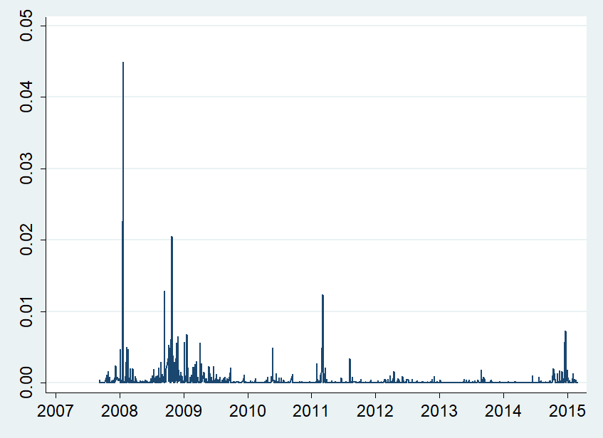
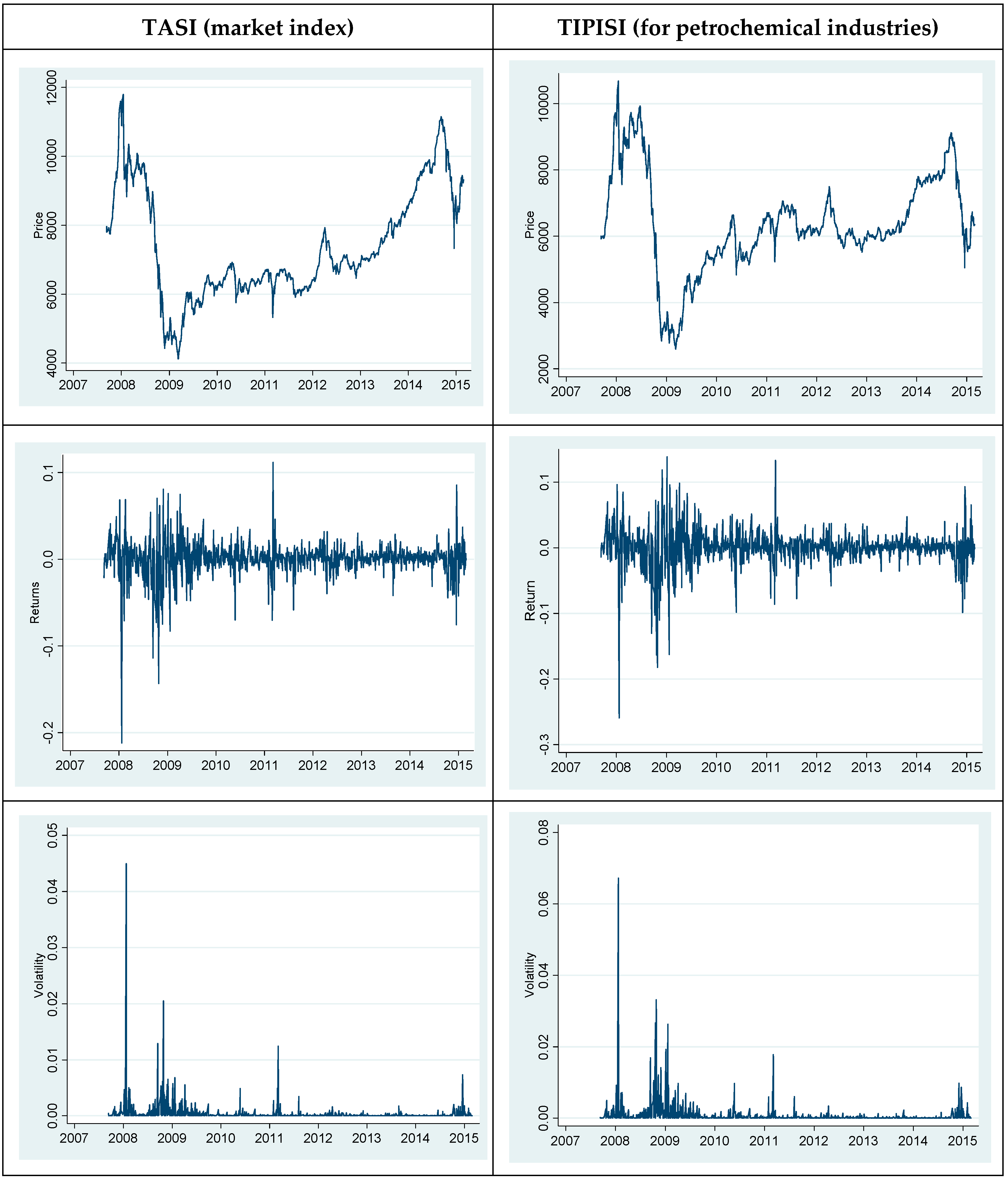
Let P_t denote the index price on day t and r_t = 100 ln (P_t/P_t−1) for t = 1, 2, …, T, where r_t is the log difference between the index prices for each index series. Following Sadorsky (2006) and Kang et al. (2009), the daily squared returns (r_t²) variable was used to measure the daily actual volatility. The graphical representation of the prices, returns, and volatility for the TASI and TIPISI are presented in Figure 2. The left panel provides the data for the TASI, and the right panel the data for the TIPISI of petrochemical industries.

Table 1. Descriptive Statistics. This table presents summary statistics for the Tadawul All Share Index (TASI) and Tadawul Industrial Petrochemical Industries Share Index (TIPISI) return series. The return indexes were obtained as the first difference of the natural logarithm. JB (Jarque–Bera) statistics is the statistics test for normality in the sample returns distribution. Q (Ljung-Box) is the statistics test of the return series for serial correlation of order 20. ADF is the statistics of the Augmented Dickey–Fuller unit root tests.

Descriptive Statistics	Tadawul All Share Index (TASI)	TIPISI for Petrochemical Industries
Mean (%)	0.014	0.005
Median (%)	0.120	0.078
Standard Deviation (%)	1.894	2.617
Minimum	−0.212	−0.259
Maximum	0.111	0.139
Skewness	−1.846	−1.468
Kurtosis	24.054	19.117
Jarque–Bera	21988.62 *	12915.59 *
Q(20)	82.080 *	69.926 *
ADF	−29.662 *	−30.139 *

* indicates rejection at the 1% significance level.

presents the summary statistics of the TASI and TIPISI return series. The table shows that the TIPISI for petrochemical industries is more volatile than the TASI. The return series for the TASI and the TIPIS are skewed to the left (i.e., negative skewness), and the return series of each exhibits high kurtosis, which suggests the presence of asymmetry. As a result, the Jarque–Bera statistics led us to reject the null hypothesis of normal distribution. The sample departures from the normal distribution are summarized by the coefficients of kurtosis and skewness. The probability density functions that can capture this phenomenon (fat tail and asymmetry) are Student-t distribution and the GED distribution.

The Ljung-Box (LB) statistics for serial correlations show that the null hypothesis of no correlation up to the 20th order is rejected, and that all of the series are serial correlated. We also checked the stationarity of the time series data by using Augmented Dickey–Fuller (ADF) tests for both indexes with the intercept, and with both intercept and trend. According to the test results, the variables are non-stationary at the level specification or indexes, but their first log differences or returns are stationary. The Augmented Dickey–Fuller unit root tests support the rejection of the null hypothesis of a unit root at a significance level of 1%, which suggests that the two return series are stationary, and can be modeled directly without any further transformation.

3.2. Methodology

Modeling and forecasting the performance of various GARCH models are becoming critical processes for businesses and policy-makers around the world. We used six linear and non-linear GARCH-class models to describe and forecast the volatility of the TASI and the TIPISI for petrochemical industries. We used GARCH, AR-GARCH, and IGARCH as the applied linear models, and EGARCH, APARCH, and GJR as the applied non-linear models. In the following section, a brief discussion of each is provided.4

3.2.1. Linear GARCH-Class Models

GARCH(1,1)

The GARCH model proposed by Bollerslev (1986) and based on the work of Engle (1982) is the most commonly used volatility model:

$$r_t=c+{\epsilon }_t$$

(1)

$${\sigma }_{{}_t}^2=\omega +\alpha {\epsilon }_{t-1}^2+{\beta }_i{\sigma }^2{}_{t-1}$$

(2)

where ${\sigma }^2{}_t$ is the conditional variance, and ${\epsilon }_{t-1}^2$ are the past squared errors from Equation (1).

AR(1)-GARCH(1,1)

The class AR(1)-GARCH(1,1) process where the mean is modeled by a first-order autoregressive AR(1) with a GARCH(1,1) error:

$$r_t=c+{\mathsf{\Phi }}_1{r}_{t-1}+{\mathsf{\Phi }}_2{r}_{t-2}+...+{\mathsf{\Phi }}_p{r}_{t-p}+{\epsilon }_t$$

(3)

$${\sigma }_{{}_t}^2=\omega +\alpha {\epsilon }_{t-1}^2+{\beta }_i{\sigma }^2{}_{t-1}$$

(4)

IGARCH

In the integrated generalized autoregressive conditional heteroskedasticity (IGARCH) model, developed by Engle and Bollerslev (1986), the sum of the parameters is 1 (i.e., α + β = 1) and the unconditional variance is infinite:

$${\sigma }_t^2=\omega +{{\displaystyle \sum }}_{i=1}^p{\alpha }_i{\epsilon }_{t-i}^2+{{\displaystyle \sum }}_{j=1}^q{\beta }_j{\sigma }_{t-j}^2$$

(5)

3.2.2. Non-Linear GARCH-Class Models

Asymmetric Power of ARCH (APARCH)

The Asymmetric Power of ARCH (APARCH) model developed by Ding et al. (1993) has been found to be particularly relevant in many recent applications (Mittnik and Paolella 2000; Giot and Laurent 2003). The APARCH(1,1) model can be defined as follows:

$${\sigma }_t^{\delta }=\omega +{{\displaystyle \sum }}_{i=1}^p{\alpha }_i{(\left|{ϵ}_{t-i}\right|-{\gamma }_i{ϵ}_{t-i})}^{\delta }+{{\displaystyle \sum }}_{j=1}^q{\beta }_j{\sigma }_{t-j}^{\delta }$$

(6)

where δ > 0, $\left|{\gamma }_i\right|\le 1$ for $i=1,\dots ,r,$ ${\gamma }_i=0$ for all $i>r$, and $r\le p$.

Note that the GJR-GARCH model can be derived or estimated from this model when δ = 2, as we will explain in the next subsection (GJR is a special case of APARCH).

GJR

Developed by Glosten, Jagannathan, and Runkle, the Glosten–Jagannathan–Runkle (GJR)-GARCH (Glosten et al. 1993) is used to model asymmetry in the ARCH process. GJR-GARCH is designed to capture the potential larger impact of negative shocks on return volatility, which is known as the asymmetric leverage volatility effect (Tenenbaum et al. 2010). The specification of the conditional variance for the GJR(1,1) model can be presented as follows:

$${\sigma }_t^2=\omega +\alpha {\epsilon }_{t-1}^2+\beta {\sigma }_{t-1}^2+\gamma {\epsilon }_{t-1}^2{I}_{t-1}$$

(7)

where $I_{t-1}=1$, if ${\epsilon }_{t-1}^2<0$ or 0 otherwise.

EGARCH

The exponential generalized autoregressive conditional heteroskedastic (EGARCH) model was developed by Nelson (1991). The shock is asymmetric when γ ≠ 0, and the exponential leverage effect is present when γ < 0. Further, the persistence of shock in the EGARCH(p,q) model is measured by Σβi:

$$\log \left({\sigma }_t^2\right)=\omega +{{\displaystyle \sum }}_{i=1}^p{\alpha }_i\left|\frac{{ϵ}_{t-i}}{{\sigma }_{t-i}}\right|+{{\displaystyle \sum }}_{j=1}^q{\beta }_j\log \left({\sigma }_{t-j}^2\right)+{{\displaystyle \sum }}_{k=1}^r{\gamma }_{k}c\frac{{\epsilon }_{t-k}}{{\sigma }_{t-k}}$$

(8)

4. Analysis of Results

We estimated six GARCH-class models—three linear models (GARCH, AR-GARCH, and IGARCH) and three non-linear models (EGARCH, APARCH, and GJR)—to describe and forecast the volatility of the TASI and the TIPISI for petrochemical industries.

Table 2. Estimation results of different volatility models on the TASI. This table presents the in-sample estimation results for the different volatility models during the period of 10 September 2007 to 3 August 2014. Panel A presents the in-sample estimation results using Student-t distribution. Panel B presents the in-sample estimation results using GED distribution. Log(L) is the logarithm maximum likelihood function value. AIC is the average Akaike information criterion. Q(20) is the Ljung-Box Q-statistic of order 20 computed on the standardized residuals. Q²(20) is the Ljung-Box Q-statistic of order 20 computed on the squared standardized residuals. Numbers in parentheses are the p-values.

TASI	GARCH		AR(1)-GARCH(1,1)		IGARCG		EGARCH		APARCH		GJR
Panel A: Student-t Distribution
ω	5.10 × 10−6	(0.000)	6.50 × 10−6	(0.067)			−0.301	(0.000)	0.000	(0.396)	6.34 × 10−6	(0.040)
α	0.199	(0.025)	0.225	(0.033)	0.066	(0.000)	−0.064	(0.046)	0.183	(0.000)	0.208	(0.016)
β	0.887	(0.000)	0.872	(0.000)	0.934	(0.000)	0.982	(0.000)	0.885	(0.000)	0.864	(0.000)
γ							0.288	(0.000)	0.276	(0.017)	0.178	(0.043)
δ									1.199	(0.000)
Log(L)	3152.14		3154.06		3138.68		3155.08		3156.80		3154.41
AIC	−6.017		−6.025		−5.996		−6.021		−6.023		−6.012
Q(20)	22.739	(0.302)	16.219	(0.819)	22.907	(0.293)	26.054	(0.198)	27.256	(0.128)	24.461	(0.262)
Q2(20)	16.790	(0.667)	17.791	(0.601)	13.944	(0.833)	14.828	(0.786)	15.124	(0.769)	13.561	(0.852)
Panel B: GED Distribution
ω	3.6 × 10−6	(0.008)	4.1 × 10−6	(0.004)			−0.344	(0.000)	0.000	(0.425)	4.35 × 10−6	(0.003)
α	0.124	(0.000)	0.136	(0.000)	0.0695	(0.000)	−0.053	(0.037)	0.1463	(0.000)	0.133	(0.000)
β	0.871	(0.000)		(0.000)	0.931	(0.000)	0.979	(0.000)	0.877	(0.000)	0.854	(0.000)
γ							0.235	(0.000)	0.305	(0.013)	0.175	(0.054)
Δ									1.058	(0.000)
Log(L)	3158.11		3158.73		3147.01		3161.41		3163.58		3160.22
AIC	−6.029		−6.034		−6.011		−6.033		−6.036		−6.031
Q(20)	22.541	(0.317)	19.946	(0.398)	20.480	(0.315)	25.665	(0.177)	27.618	(0.119)	24.366	(0.227)
Q2(20)	16.587	(0.680)	16.910	(0.659)	13.171	(0.870)	14.409	(0.809)	15.454	(0.750)	13.516	(0.854)

presents the in-sample estimation results for the different volatility models of TASI using the Student-t distribution (Panel A) and the GED distribution (Panel B). Table 2 also presents the results of the diagnostic test for the standardized residuals. Table 2 (Panel A and Panel B) also shows that the β coefficients of all the stocks are statically significant, which indicates that Saudi stocks are subject to time-clustering volatility. It is shown also that β is close to one for IGARCH and EGARCH, and significant at the 1% level. That is, there is a high degree of volatility persistence in the Saudi stock market. Further, the coefficients of all of the GARCH models are significant at all significance levels, which indicates that all of the models have a high level of validity.

We used log likelihood and AIC to determine the distribution (i.e., Student-t distribution and GED distribution) that fits the data the best. Table 2 (Panel A and Panel B) indicates that the GED distribution has the highest log likelihood value and the lowest AIC value of all the GARCH-class models relative to the Student-t distribution, which means that the GED distribution fits the TASI data better than the Student-t distribution does. This will be important in our discussion of the forecasting accuracy criteria of the TASI.

Table 3. Estimation results of different volatility model on the TIPISI. This table presents the in-sample estimation results for the different volatility models during the period of 10 September 2007 to 3 August 2014. Panel A presents the in-sample estimation results using Student-t distribution. Panel B presents the in-sample estimation results using GED distribution. Log(L) is the logarithm maximum likelihood function value. AIC is the average Akaike information criterion. Q(20) is the Ljung-Box Q-statistic of order 20 computed on the standardized residuals. Q²(20) is the Ljung-Box Q-statistic of order 20 computed on the squared standardized residuals. Numbers in parentheses are the p-values.

TIPISI	GARCH		AR(1)-GARCH(1,1)		IGARCG		EGARCH		APARCH		GJR
Panel A: Student-t Distribution
Ω	4.8 × 10−6	(0.097)	1.6 × 10−6	(0.094)			−0.224	(0.000)	0.000	(0.502)	5.58 × 10−6	(0.081)
Α	0.160	(0.016)	0.181	(0.029)	0.060	(0.000)	−0.039	(0.170)	0.159	(0.000)	0.166	(0.015)
Β	0.909	(0.000)	0.902	(0.000)	0.940	(0.000)	0.989	(0.000)	0.909	(0.000)	0.903	(0.000)
γ							0.266	(0.000)	0.181	(0.103)	0.098	(0.218)
Δ									1.233	(0.000)
Log(L)	2810.233		2809.160		2800.40		2811.54		2812.91		2811.04
AIC	−5.364		−5.365		−5.349		−5.364		−5.365		−5.363
Q(20)	18.858	(0.531)	16.667	(0.612)	20.608	(0.421)	18.994	(0.522)	18.725	(0.540)	18.693	(0.805)
Q2(20)	23.227	(0.278)	24.223	(0.233)	21.765	(0.353)	22.036	(0.339)	21.514	(0.367)	22.098	(0.333)
Panel B: GED Distribution
ω	7.3 × 10−6	(0.031)	5.3 × 10−6	(0.000)			−0.262	(0.000)	0.000	(0.490)	4.20 × 10−6	(0.024)
α	0.100	(0.000)	0.106	(0.000)	0.066	(0.000)	−0.024	(0.279)	0.129	(0.000)	0.104	(0.000)
β	0.900	(0.000)	0.881	(0.000)	0.934	(0.000)	0.986	(0.000)	0.897	(0.000)	0.895	(0.000)
γ							0.219	(0.000)	0.194	(0.099)	0.065	(0.378)
δ									0.933	(0.004)
Log(L)	2805.0		2746.83		2798.96		2808.01		2809.16		2806.053
AIC	−5.355		−5.248		−5.346		−5.358		−5.358		−5.325
Q(20)	18.569	(0.500)	14.145	(0.775)	20.333	(0.437)	18.521	(0.553)	18.240	(0.572)	18.532	(0.552)
Q2(20)	23.357	(0.272)	25.485	(0.183)	20.710	(0.414)	22.391	(0.320)	21.828	(0.350)	22.638	(0.307)

presents the in-sample estimation results for the different volatility models of the TIPISI of the petrochemical industries using the Student-t distribution (Panel A) and the GED distribution (Panel B). The table shows that β is close to one for IGARCH and EGARCH with significance at the 1% level. This means that there is a high degree of volatility persistence in the Saudi stock market. In addition, the coefficients of almost all the GARCH models are statistically significant, which suggests that the models have a high level of validity.

We also applied log likelihood and Akaike information criterion (AIC) to determine the distribution that fits the TIPISI data best. Table 2 (Panel A and Panel B) indicates that the Student-t distribution has the highest log likelihood value and the lowest AIC for all the GARCH-class models relative to the GED distribution, which means that the Student-t distribution fits the TIPISI data better than the GED distribution does.

We adopted three loss functions as the forecasting criteria (Poon and Granger 2003): the Mean Square Error (MSE), the Mean Absolute Error (MAE), and the Mean Absolute Percentage Error (MAPE). We considered these criteria in assessing the forecasting accuracy of the GARCH-class models.

Table 4. Evaluation of one-day out-of-sample volatility forecasts comparison for TASI. The table presents the loss functions values of TASI. Panel A displays the loss functions values for one-day out-of-sample volatility forecasts of TASI using Student-t distribution. Panel B displays the loss functions’ values for one-day out-of-sample volatility forecasts of TASI using GED distribution. This table also presents the forecasting criteria: Mean Square Error (MSE), Mean Absolute Error (MAE), and Mean Absolute Percentage Error (MAPE). Lowest values for the statistics are denoted in bold face. GARCH: generalized autoregressive conditional heteroskedasticity, AR-GARCH: autoregressive GARCH, IGARCH: integrated GARCH, EGARCH: exponential GARCH, APARCH: Asymmetric Power of ARCH, GJR: Glosten–Jagannathan–Runkle.

Base Model for TASI	Mean Square Error (MSE)	Mean Absolute Error (MAE)	Mean Absolute Percentage Error (MAPE)
Panel A: with Student-t Distribution
GARCH(1,1)	0.020188	0.013079	174.3824
AR(1)-GARCH(1,1)	0.020190	0.013080	176.3826
IGARCH	0.020188	0.013079	174.4758
EGARCH	0.020180	0.013073	168.7434
APARCH	0.020179	0.013072	167.7398
GJR	0.020181	0.013074	169.4914
Panel B: with GED Distribution
GARCH(1,1)	0.020189	0.013080	174.6468
AR(1)-GARCH(1,1)	0.020193	0.013083	178.3879
IGARCH	0.020188	0.013080	174.5719
EGARCH	0.020184	0.013076	171.3569
APARCH	0.020181	0.013074	169.2901
GJR	0.020184	0.013076	171.7368

presents the values of these forecasting accuracy criteria for the out-of-sample TASI forecasts at the one-day forecasting horizon. The first column in this table lists the base models (i.e., the conditional volatility models). Based on various forecasting criteria or loss functions, APARCH, followed by EGARCH, was the model that performed best for the TASI with the lowest value on all three criteria regardless of the non-Gaussian distribution. In sum, our results show that the non-linear GARCH-class models, and specifically the APARCH model, are more effective than the linear models for capturing the short-run dynamics of the TASI’s volatility.

Table 5. Evaluation of one-day out-of-sample volatility forecasts comparison for the TIPISI. The table presents the loss functions values of the TIPISI. Panel A displays the loss functions values for one-day out-of-sample volatility forecasts of the TIPISI using Student-t distribution. Panel B displays the loss functions values for one-day out-of-sample volatility forecasts of the TIPISI using GED distribution. This table also presents the forecasting criteria: Mean Square Error (MSE), Mean Absolute Error (MAE), and Mean Absolute Percentage Error (MAPE). Lowest values for the statistics are denoted in bold face.

Base Model for TIPISI	Mean Square Error (MSE)	Mean Absolute Error (MAE)	Mean Absolute Percentage Error (MAPE)
Panel A: with Student-t Distribution
GARCH(1,1)	0.026567	0.017486	126.0563
AR(1)-GARCH(1,1)	0.026570	0.017487	126.8104
IGARCH	0.026567	0.017486	126.1189
EGARCH	0.026565	0.017485	125.6517
APARCH	0.026563	0.017482	124.9681
GJR	0.026560	0.017480	124.3673
Panel B: with GED Distribution
GARCH(1,1)	0.026544	0.017466	120.1382
AR(1)-GARCH(1,1)	0.026584	0.017498	130.4249
IGARCH	0.026531	0.017453	116.3927
EGARCH	0.026544	0.017466	120.1388
APARCH	0.026544	0.017466	120.1066
GJR	0.026532	0.017446	114.3430

presents the values of the forecasting accuracy criteria for the out-of-sample TIPISI forecasts at the one-day forecasting horizon using the Student-t distribution (Panel A) and the GED distribution (Panel B). Panel A shows that GJR, followed by APARCH, was the model with the best performance for the TIPISI of the petrochemical industries on all three criteria. Panel B shows that IGARCH, followed by GJR, was the model with the best performance on the TIPISI of the petrochemical industries on two of the three criteria. Note that the GED distribution for the TIPISI is not of interest, as the Student-t distribution fits the TIPISI data better than the GED distribution does. That is, GJR is the most accurate model for forecasting the volatility of the TIPISI for the petrochemical industries.

The major results up to this point indicate that the APARCH model is the most accurate for forecasting the volatility of the TASI, given that this model outperforms the others in evaluating model estimation. However, for forecasting volatility, we used an in-sample period of both high and low volatility to forecast a period of moderate volatility. Would the results be the same if we had excluded periods of high volatility (i.e., 2007, 2008, and the first half of 2009, as shown in Figure 2)? To answer this question, we reproduced Table 4 and Table 5, and found that the results are still valid. In more detail, Table 4 was reproduced after excluding the financial crisis and Saudi Arabia’s stock collapse periods (i.e., from January 2007 to June 2009). We used the data from 1 July 2009 to 3 August 2014 to evaluate the in-sample data for volatility modeling. Based on the various loss functions (

Table 6. Evaluation of one-day out-of-sample volatility forecasts comparison for the TASI after excluding the high volatility periods. The table presents the loss function values for one-day out-of-sample volatility forecasts of TASI. This table is a reproduction of Table 4 after excluding the financial crisis period and Saudi Arabia’s stock collapse period. We used the data from 1 July 2009 to 3 August 2014 to evaluate in-sample data for volatility modeling. This table also presents the forecasting criteria: Mean Square Error (MSE), Mean Absolute Error (MAE), and Mean Absolute Percentage Error (MAPE). Lowest values for the statistics are denoted in bold face.

Base Model for TASI	Mean Square Error (MSE)	Mean Absolute Error (MAE)	Mean Absolute Percentage Error (MAPE)
Panel A: with Student-t Distribution
GARCH(1,1)	0.020182	0.013074	169.9660
AR(1)-GARCH(1,1)	0.020179	0.013071	168.6884
IGARCH	0.020176	0.013071	165.7842
EGARCH	0.020169	0.013068	160.9874
APARCH	0.020167	0.013067	159.5988
GJR	0.020169	0.013068	161.0318
Panel B: with GED Distribution
GARCH(1,1)	0.020184	0.013076	171.3374
AR(1)-GARCH(1,1)	0.020180	0.013073	169.2373
IGARCH	0.020181	0.013074	169.2680
EGARCH	0.020174	0.013070	164.6818
APARCH	0.020173	0.013069	163.8528
GJR	0.020175	0.013070	164.8143

) of all the models, APARCH performed the best for the TASI with the lowest value on all three criteria, regardless of the non-Gaussian distribution. In other words, these results further confirm that the APARCH model is more effective than the linear models at capturing the short-run dynamics of TASI volatility.

In terms of the TIPISI for the petrochemical industries, the major results based on the full sample indicate that the GJR model is the most accurate for forecasting TIPISI volatility (see

Table 7. Evaluation of one-day out-of-sample volatility forecasts comparison for the TIPISI after excluding the high volatility periods. The table presents the loss function values for the one-day out-of-sample volatility forecasts of the TIPISI. This table is a reproduction of Table 5 after excluding the financial crisis period and Saudi Arabia’s stock collapse period. We used data from 1 July 2009 to 3 August 2014 to evaluate in-sample data for volatility modeling. This table also presents the forecasting criteria: Mean Square Error (MSE), Mean Absolute Error (MAE), and Mean Absolute Percentage Error (MAPE). Lowest values for the statistics are denoted in bold face.

Base Model for TIPISI	Mean Square Error (MSE)	Mean Absolute Error (MAE)	Mean Absolute Percentage Error (MAPE)
Panel A: with Student-t Distribution
GARCH(1,1)	0.026561	0.017481	124.5730
AR(1)-GARCH(1,1)	0.026557	0.017476	123.5319
IGARCH	0.026559	0.017479	124.0390
EGARCH	0.026557	0.017477	123.4998
APARCH	0.026555	0.017476	123.0528
GJR	0.026556	0.017477	123.3397
Panel B: with GED Distribution
GARCH(1,1)	0.026522	0.017446	114.0507
AR(1)-GARCH(1,1)	0.026622	0.017530	139.6749
IGARCH	0.026521	0.017444	113.6684
EGARCH	0.026521	0.017444	113.6853
APARCH	0.026521	0.017444	113.6685
GJR	0.026521	0.017444	113.6540

). In order to check robustness, we reproduced Table 5 after excluding the financial crisis period and Saudi Arabia’s stock collapse period. According to our results for all the models, APARCH performed the best for the TIPISI of petrochemical industries on all three of the criteria. It is worth noting that the GED distribution of the TIPISI index is not of interest, as the Student-t distribution fits the TIPISI data better than the GED distribution. These results confirm that the APARCH and GJR (which is a special case of APARCH) models are more effective than the linear models for capturing the short-run dynamics of the TIPISI.

Finally, it is worth noting that the differences presented in the loss functions for APARCH, EGARCH, and GJR are very small, which may indicate that these models are as good as the others. To test for that, we perform Diebold–Mariano test to compare the predictive accuracy between two forecast methods (with a null hypothesis that the forecast accuracy is equal). For the full sample, the Diebold–Mariano test results (see

Table 8. Diebold–Mariano test for forecast comparison of the TASI and TIPISI for the full sample. The table presents the Diebold–Mariano test for the full sample (10 September 2007 to 3 August 2014) using Student-t and GED distribution. Panel A displays the Diebold–Mariano test for the TASI using Student-t and GED distribution. Panel B displays the Diebold–Mariano test for the TIPISI using Student-t and GED distribution. Numbers in parentheses are the p-values.

	Student-t Distribution		GED Distribution
	Diebold–Mariano Test	Better Forecast	Diebold–Mariano Test	Better Forecast
Panel A: TASI
APARCH, GARCH	−0.8504 (0.3951)	APARCH	−0.8623 (0.3885)	APARCH
APARCH, GJR	−0.8525 (0.3939)	APARCH	−0.8634 (0.3879)	APARCH
Panel B: TIPISI
APARCH, EGARCH	−1.365 (0.1722)	APARCH	−1.310 (0.1902)	APARCH
APARCH, GJR	1.358 (0.1743)	GJR	1.279 (0.2008)	GJR

) indicate the superiority of APARCH over EGARCH and GJR for the TASI and the superiority of GJR for the TIPISI.

As for the period of 1 July 2009 to 3 August 2014 (i.e., after excluding the period of high volatility), the Diebold–Mariano test results (see

Table 9. Diebold–Mariano test for forecast comparison of the TASI and TIPISI after excluding periods of high volatility. The table presents Diebold–Mariano test from 1 July 2009 to 3 August 2014 using Student-t and GED distribution. Panel A displays the Diebold–Mariano test for the TASI using Student-t and GED distribution. Panel B displays the Diebold–Mariano test for TIPISI using Student-t and GED distribution. Numbers in parentheses are the p-values.

	Student-t Distribution		GED Distribution
	Diebold–Mariano Test	Better Forecast	Diebold–Mariano Test	Better Forecast
Panel A: TASI
APARCH, EGARCH	−0.8027 (0.4221)	APARCH	−0.8267 (0.4084)	APARCH
APARCH, GJR	−0.8029 (0.4221)	APARCH	−0.8271 (0.4082)	APARCH
Panel B: TIPISI
APARCH, EGARCH	−1.344 (0.1791)	APARCH	−1.241 (0.2145)	APARCH
APARCH, GJR	−1.343 (0.1793)	APARCH	1.241 (0.2146)	GJR

) show that the APARCH model performs better than the EGARCH and GJR models for the TASI under the GED distribution. As for the TIPISI, the Diebold–Mariano test shows the superiority of the APARCH model under the Student-t distribution. In sum, the Diebold–Mariano test results are in line with our findings regarding the best fit model for both the TASI and TIPISI data.

After finding the best models for each index, we provided a further application for testing the forecasted volatility values. In fact, understanding modeling and forecasting performance is relevant for investment portfolio management and hedging against risk. This paper contributes to the field by providing the investment community with a model for assessing and forecasting the risk attendant upon investing in the Saudi stock market. For example, with these results, investors are better informed about the petrochemical industry stocks in their portfolio profiles, which is an important consideration, given the need to model and forecast daily returns volatility, as optimal decision making relies on understanding how returns can fluctuate over a given time horizon. Put differently, based on this study, investors can avail themselves of information to support accurate decision making in terms of their investments and portfolio diversification.

5. Conclusions

In this paper, we focused on the econometric modeling of volatility and the family of GARCH-class models for the Saudi stock market. Our purpose was to evaluate the forecasting performance of linear and non-linear generalized autoregressive conditional heteroskedasticity (GARCH)-class models in terms of their in-sample and out-of-sample forecasting accuracy for the Saudi stock market index, TASI, and the TIPISI for petrochemical industries. In other words, we made contributed to addressing the gap in the literature by identifying the volatility model that outperforms other models in terms of in-sample and out-of-sample forecasting accuracy for the Saudi stock market.

We compared the forecasting performance of several GARCH models in regard to out-of-sample forecast ability. The GARCH models were evaluated based on their ability to forecast future returns. According to the results obtained by the three loss functions—MSE, MAE, and MAPE—we concluded that the most appropriate models for modeling the volatility of TIPISI for the full sample and after excluding periods of high volatility are GJR and APARCH, respectively. We also conclude that the APARCH model is the most accurate for forecasting the volatility of TASI for the full sample and after excluding periods of high volatility. These results are also confirmed by these obtained from the Diebold–Mariano test.

These results are also confirmed; that is, non-linear GARCH-class models can provide a good approximation for capturing the TASI and TIPISI for petrochemical industries. This finding is robust, even when the financial crisis and Saudi Arabia’s stock collapse period are excluded from the data. Furthermore, the results of this study support those of previous studies, in which it is concluded that compared with linear GARCH-class models, non-linear GARCH-class models are a better fit for measuring the volatility of stock market returns (e.g., Gabriel 2012; Al Rahahleh 2017).

The practical implication of our results are that traders in the Saudi stock market might consider these models in understanding risk in the petrochemical industries and the riskiness of the Saudi stock market in general, which may help them in their approach to risk management strategies for the daily stock market index returns. Further, these results imply that the APARCH model might be more useful than other models when implementing risk management strategies and developing stock pricing model.

As modeling and forecasting the performance of various GARCH models are becoming critical processes for businesses and policy-makers around the world, our results are of benefit to policy-makers in predicting the riskiness of the two indices examined herein.

References

- Al Freedi, Ajab, Ahmed Shamiri, and Zaidi Isa. 2012. A Study on the Behavior of Volatility in Saudi Arabia Stock Market Using Symmetric and Asymmetric GARCH Models. Journal of Mathematics and Statistics 8: 98–106. [Google Scholar]
- Al Rahahleh, Naseem. 2017. Modelling and Forecasting Equity Markets Volatility: An Empirical Evidence. Journal of Applied Statistical Science 22: 387–405. [Google Scholar]
- Almohaimeed, Ahmed, and Nizar Harrathi. 2013. Volatility Transmission and Conditional Correlation between Oil prices, Stock Market and Sector Indexes: Empirics for Saudi Stock Market. Journal of Applied Finance & Banking 3: 125–41. [Google Scholar]
- Basher, Syed A., and Perry Sadorsky. 2006. Oil Price Risk and Emerging Stock Markets. Global Finance Journal 17: 224–51. [Google Scholar] [CrossRef]
- Bollerslev, Tim. 1986. Generalized autoregressive conditional heteroskedasticity. Journal of Econometrics 31: 307–27. [Google Scholar] [CrossRef]
- Carvalho, Marcelo C., Marco Aurélio Freire, Marcelo C. Medeiros, and Leonardo R. Souza. 2006. Modelling and Forecasting the Volatility of Brazilian Asset Returns: A Realized Variance Approach. Brazilian Review of Finance 4: 321–43. [Google Scholar]
- Ding, Zhuanxin, Clive W. J. Granger, and Robert F. Engle. 1993. A Long Memory Property of Stock Market Returns and a New Model. Journal of Empirical Finance 1: 83–106. [Google Scholar] [CrossRef]
- Engle, Robert F. 1982. Autoregressive Conditional Heteroskedasticity with Estimates of the Variance of United Kingdom Inflation. Econometrica 50: 987–1007. [Google Scholar] [CrossRef]
- Engle, Robert F. 2001. GARCH 101: The Use of ARCH/GARCH Models in Applied Econometrics. Journal of Economic Perspectives 15: 157–68. [Google Scholar] [CrossRef]
- Engle, Robert F., and Tim Bollerslev. 1986. Modelling the persistence of conditional variances. Econometric Reviews 5: 1–50. [Google Scholar] [CrossRef]
- Engle, Robert F., and Victor K. Ng. 1993. Measuring and testing the impact of news on volatility. The Journal of Finance 48: 1749–78. [Google Scholar] [CrossRef]
- Figlewski, Stephen. 2004. Forecasting Volatility. Working Paper. New York, NY, USA: New York University Stern School of Business. [Google Scholar]
- Fornari, Fabio, and Antonio Mele. 2009. Financial Volatility and Economic Activity. Working Paper. London, UK: London School of Economics. [Google Scholar]
- Franses, Philip Hans, and Dick van Dijk. 1996. Forecasting Stock Market Volatility Using (Non-Linear) GARCH Models. Journal of Forecasting 15: 229–35. [Google Scholar] [CrossRef]
- Gabriel, Anton Sorin. 2012. Evaluating the Forecasting Performance of GARCH Models Evidence from Romania. Procedia Social and Behavioral Sciences 62: 1006–10. [Google Scholar] [CrossRef]
- Giot, Pierre, and Sebastien Laurent. 2003. Market Risk in Commodity Markets: A VaR Approach. Energy Economics 25: 435–57. [Google Scholar] [CrossRef]
- Glosten, Lawrence R., Ravi Jagannathan, and David E. Runkle. 1993. On the Relation between the Expected Value and the Volatility of the Nominal Excess Return on Stocks. Journal of Finance 48: 1779–801. [Google Scholar] [CrossRef]
- Hamadu, Dallah, and Ade Ibiwoye. 2010. Modeling and Forecasting the Volatility of the Daily Returns of Nigerian Insurance Stocks. International Business Research 3: 106–16. [Google Scholar] [CrossRef]
- Hammoudeh, Shawkat, and Eisa Aleisa. 2004. Dynamic Relationship among GCC Stock Markets and NYMEX Oil Futures. Contemporary Economic Policy 22: 250–69. [Google Scholar] [CrossRef]
- Hammoudeh, Shawkat, and Huimin Li. 2008. Sudden Changes in Volatility in Emerging Markets: The Case of Gulf Arab Stock Markets. International Review of Financial Analysis 17: 47–63. [Google Scholar] [CrossRef]
- Kalyanaraman, Lakshmi. 2014. Stock Market Volatility in Saudi Arabia: An Application of Univariate GARCH Model. Asian Social Science 10: 142–52. [Google Scholar] [CrossRef]
- Kang, Sang Hoon, Sang-Mok Kang, and Seong-Min Yoon. 2009. Forecasting Volatility of Crude Oil Markets. Energy Economics 31: 119–25. [Google Scholar] [CrossRef]
- Kovačić, Zlatko J. 2007. Forecasting Volatility: Evidence from the Macedonian Stock Exchange. Munich Personal RePEc Archive, MPRA, Paper No. 5319. Available online: https://mpra.ub.uni-muenchen.de/5319/1/MPRA_paper_5319.pdf (accessed on 25 August 2017).
- McMillan, David N., Alan Speight, and Owain Apgwilym. 2000. Forecasting UK stock market volatility. Applied Financial Economics 10: 435–48. [Google Scholar] [CrossRef]
- Mittnik, Stefan, and Marc S. Paolella. 2000. Conditional Density and Value-at-Risk Prediction of Asian Currency Exchange Rates. Journal of Forecasting 19: 313–33. [Google Scholar] [CrossRef]
- Mohanty, Sunil K., Mohan Nandha, Abdullah Q. Turkistani, and Muhammed Y. Alaitani. 2011. Oil Price Movements and Stock Market Returns: Evidence from Gulf Cooperation Council (GCC) countries. Global Finance Journal 22: 42–55. [Google Scholar] [CrossRef]
- Nelson, Daniel B. 1991. Conditional Heteroskedasticity in Asset Returns: A New Approach. Econometrica 59: 347–70. [Google Scholar] [CrossRef]
- Ng, Hock Guan, and Michael McAleer. 2004. Recursive modelling of symmetric and asymmetric volatility in the presence of extreme observations. International Journal of Forecasting 20: 115–29. [Google Scholar] [CrossRef]
- Onour, Ibrahim. 2007. Impact of oil price volatility on Gulf Cooperation Council Stock Markets’ Return. OPEC Review 31: 171–89. [Google Scholar] [CrossRef]
- Patev, Plamen, and Nigokhos Kanaryan. 2008. Stock Market Volatility Changes in Central Europe Caused by Asian and Russian Crisis. International Journal of Economic Research 5: 13–35. [Google Scholar]
- Patev, Plamen, and Nigokhos Kanaryan. 2009. Modelling and Forecasting the Volatility of Thin Emerging Stock Markets: The Case of Bulgaria. Comparative Economic Research 12: 47–60. [Google Scholar] [CrossRef]
- Poon, Ser-Huang, and Clive W. J. Granger. 2003. Forecasting Volatility in Financial Markets: A Review. Journal of Economic Literature 41: 478–539. [Google Scholar] [CrossRef]
- Sadorsky, Perry. 2006. Modeling and forecasting Petroleum Futures Volatility. Energy Economics 28: 467–88. [Google Scholar] [CrossRef]
- Sedik, Tahsin Saadi, and Oral H. Williams. 2011. Global and Regional Spillovers to GCC Equity Markets. IMF Working Paper 11/138. Washington, DC, USA: International Monetary Fund. [Google Scholar]
- Tenenbaum, Joel, Davor Horvatić, Slavica Cosović Bajić, Bećo Pehlivanović, Boris Podobnik, and H. Eugene Stanley. 2010. Comparison between Response Dynamics in Transition Economies and Developed Countries. Physical Review E 82: 046104. [Google Scholar] [CrossRef] [PubMed]
- Wei, Yu, Yudong Wang, and Dengshi Huang. 2010. Forecasting Crude Oil Market Volatility: Further Evidence Using GARCH-Class. Energy Economics 32: 1477–84. [Google Scholar] [CrossRef]