Sentiment-Induced Bubbles in the Cryptocurrency Market

1
Adam Smith Business School, University of Glasgow, Glasgow G12 8QQ, UK
2
Louvain Institute of Data Analysis and Modeling, Université catholique de Louvain, 1348 Louvain-la-Neuve, Belgium
*
Author to whom correspondence should be addressed.
J. Risk Financial Manag. 2019, 12(2), 53; https://doi.org/10.3390/jrfm12020053
Submission received: 18 January 2019
/
Revised: 24 March 2019
/
Accepted: 28 March 2019
/
Published: 1 April 2019
(This article belongs to the Special Issue Alternative Assets and Cryptocurrencies)
Abstract
:Cryptocurrencies lack clear measures of fundamental values and are often associated with speculative bubbles. This paper introduces a new way of testing for speculative bubbles based on StockTwits sentiment, which is used as the transition variable in a smooth transition autoregression. The model allows for conditional heteroskedasticity and fat tails of the conditional distribution of the error term, and volatility may depend on the constructed sentiment index. We apply the model to the CRIX index, for which several bubble periods are identified. The detected locally explosive price dynamics, given the specified bubble regime controlled by a smooth transition function, are more akin to the notion of speculative bubble that is driven by exuberant sentiment. Furthermore, we find that volatility increases as the sentiment index decreases, which is analogous to the commonly called leverage effect.
JEL Classification:
C14; C43; Z111. Introduction
The current literature on bubble tests is confronted with the difficulty to conclude that a price bubble is not caused by time-varying or regime switching fundamentals (Gürkaynak 2008). Recent tests proposed by (Phillips et al. 2011, 2015) provide powerful tests, essentially based on the supremum of sequential unit root test statistics, and have been applied to the cryptocurrency markets by (Cheung et al. 2015; Corbet et al. 2018; Hafner 2018), where the latter accounts for time-varying volatility. These tests, however, are purely statistical in nature and do not allow us to infer if structural breaks detected in the time series processes of asset prices are evidence of bubbles or are due to breaks in the underlying (unobserved) fundamentals (Pesaran and Johnsson 2018). An inclusion of extracted sentiment information, representing the sentiment in the crypto community with their specific linguistic features, contributes to solving this inconclusive puzzle and adds economic and behavioral information into the statistical settings.
Alternative bubble tests have been proposed e.g., by Pavlidis et al. (2017) based on the gap between spot and futures prices and applied to equities and exchange rates, and Pavlidis et al. (2018) using market expectations of futures prices applied to the oil market—see also Kruse and Wegener (2019). With the lack of liquidity in futures prices of cryptocurrencies, it seems difficult to apply these tests to crypto markets today. Further bubble tests include Cheah and Fry (2015), who use a continuous time model to identify bubbles via anomalous behaviors of the drift and volatility components, and Fry and Cheah (2016), who develop models for financial bubbles and crashes based on statistical physics, with applications to Bitcoin and Ripple.
Bubbles are more prone to emerge in the crypto market than in the stock markets. Theoretical grounds for market efficiency rely crucially on the stabilizing powers of rational speculation—see e.g., (De Long et al. 1990; Glosten and Milgrom 1985; Yang and Brown 2016). Given the presence of limits to arbitrage (e.g., no short-sale venue) and the limited fundamental information in the cryptocurrency market, rational speculation that pulls prices close to its fundamental value is not possible. These constraints result in a hurdle of price discovery.
In this paper, we postulate that a bubble-like behavior of prices is characterized by a smooth transition function that dynamically assigns the probability (loading) to the explosive regime and the random walk regime, given the exogenous sentiment information. By this construction, the speculative bubble can only be pumped up with anomalous sentiment. We therefore develop an econometric framework and a test for a sentiment-induced price bubble.
We target the cryptocurrency-related messages in Stocktwits which attracts the crypto community to share their information, opinions and sentimental moods. We use the sentiment measures constructed by Nasekin and Chen (2018) from this social media as their newly constructed sentiment index is viewed as a representative sentiment from the crypto community, with a consideration of their specific linguistic features. The information content of it is relevant for future market performance and can be used to predict the price and volatility evolution (Chen et al. 2018). As mentioned before, due to the limited knowledge of a fundamental value in this new digital asset class, the mispricing caused by sentiments cannot be promptly corrected or revert to its fundamental value. This is the reason why sentiment entails a short-run predictability because of an inefficient crypto market that defers a price correction process. This slow correction makes sentiment accumulated and amplified; as a consequence, the bubble is able to grow and probably collapse once sentimental bias is finally being corrected.
The econometric framework is that of a smooth transition autoregressive model (STAR), where the transition variable is the sentiment index. The idea is that, in times of a very high sentiment index, corresponding to excessively bullish evaluations, the price dynamics will be driven by an explosive autoregression, while otherwise they follow a random walk. We allow for conditional heteroskedasticity and fat tails by specifying recently proposed score-driven models that are shown to fit the data well. Volatility is allowed to depend explicitly on the sentiment index. This complements previous studies on cryptocurrency volatility as in (Conrad et al. 2018; Kjaerland et al. 2018).
We apply the model to the CRIX index, which is a value weighted index of the cryptocurrency market with endogenously determined number of constituents using statistical criteria. The reallocation of the CRIX happens on a monthly and quarterly basis—see (Trimborn and Härdle 2018) and thecrix.de for details. We identify several bubble periods, primarily in 2017. Volatility is negatively depending on the sentiment index, meaning that bad sentiments or news increase volatility, a feature commonly called leverage effect in classical financial markets. Here, the leverage effect is explicitly driven by the sentiment index.
2. Cryptocurrencies and a Sentiment Index
For the task of sentiment quantification and construction, this section outlines the dataset being analyzed and the methodologies employed for quantification.
2.1. StockTwits Data
StockTwits1 is a social microblogging platform where investors and traders dedicate to financial and economic discussion. Each message, by StockTwits policy, should start with “cashtag” that explicitly refers to the specific financial asset. Through it, one can easily link the message content with the asset symbol starting with cashtag; subsequently, associate the symbol with the sentiment of message content, after textual analysis. Sentiment analysis is very possible in StockTwits due to its add-in sentiment disclosure applied to each users. Users can also express their sentiment by labeling their messages as “Bearish” (negative) or “Bullish” (positive) via a toggle button. The available labeled data benefits an advance on textual analysis that typically relies on the available training dataset.
Since 2014, StockTwits adds streams and symbology for cryptocurrencies and tokens, expanding from 100 cryptos in the beginning to more than 400 cryptos recently. This brand new and vibrant new asset class have successfully attracted a huge attention from its big community and also from new comers. New cryptocurrencies are regularly added to the list of cashtags supported by StockTwits.2 A cashtag refers to a cryptocurrency if and only if it ends with “.X” (e.g., $BTC.X for Bitcoin, $LTC.X for Litecoin). We use this convention and StockTwits Application Programming Interface (API) to download all messages containing a cashtag referring to a cryptocurrency. StockTwits API also provides for each message its user’s unique identifier, the time it was posted at with a one-second precision, and the sentiment associated by the user (“Bullish”, “Bearish” or unclassified). Our final dataset contains 1,220,728 messages from 33,613 distinct users, posted between March 2013 and May 2018, and related to 425 cryptocurrencies. Overall, 472,255 messages are classified as bullish (38.6%) and 92,033 as bearish (7.5%), and the remaining are unclassified. An imbalance between the numbers of positive and negative messages shows that online investors are optimistic on average, as previously found by (Avery et al. 2016; Kim and Kim 2014).
StockTwits, with a focus on financial discussion, offers an advantage to extract the speculative sentiment, which may ultimately trigger a speculative bubble. Another advantage is that the availability of labeled sentiment by users themselves, rendering an application of supervised learning schemes. The detail of statistical learning model applied to Stocktwits dataset will be documented in the following subsection.
2.2. Sentiment Prediction
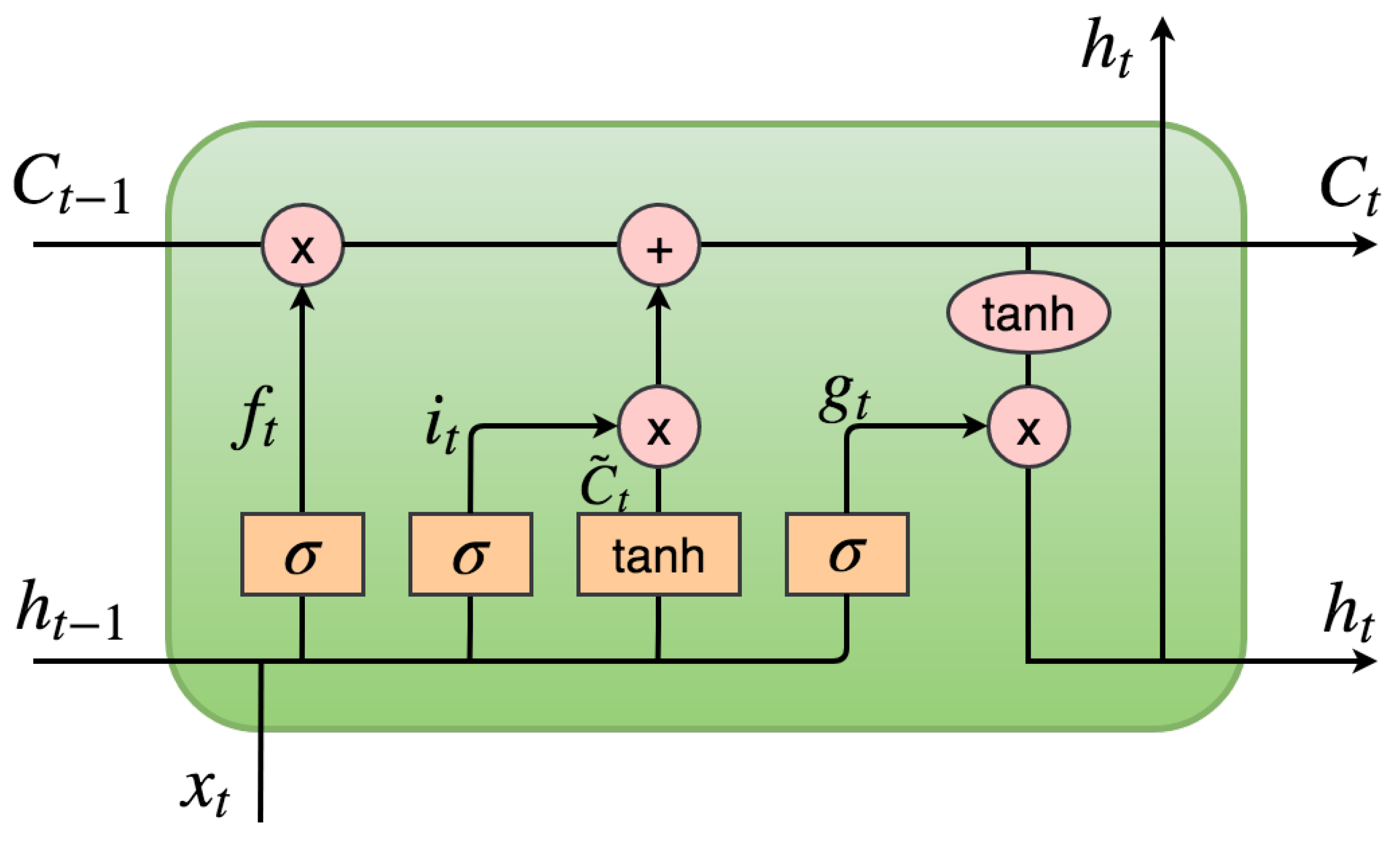
Nasekin and Chen (2018) propose a state-of-art methodology for semantic sentiment prediction in the cryptocurrency domain. The long short-term memory (LSTM) type of recurrent neural network (RNN), together with word embedding technique provide a superior performance in predicting domain-specific sentiment. The key advantageous feature in the LSTM is to keep the context-specific dependence encoded, so that the important information about semantic structure of sentence won’t be lost.
A general architecture of a sentiment prediction LSTM/RNN network is presented in Figure 1 of Nasekin and Chen (2018). This architecture consists of the input sequence, an embedding lookup matrix, several layers of LSTM cells/units, an output sequence, mean pooling and softmax layers. The core of this structure are the LSTM cells. The structure of these cells is presented in Figure 1. The specifications of this structure include several steps: (1) introducing the cell state to keep information about the previous states of LSTM cells. The amount of information stored in the cell state is controlled by the “gates”: an input gate , a forget gate and an output gate . The first to act is the forget gate : it determines how much of the previous state will be kept based on the values of the previous hidden state and the current input . The sigmoid function outputs a value between 0 and 1 for each number in the cell state ; (2) generating an update to through a new candidate value of the cell state, , and deciding how much of the new candidate state will be inputted into ; and (3) updating the value of the cell state as a weighted sum of the previous cell state value and the new candidate value ; (4) updating the the hidden state as a filtered value of the cell state , which is put through the tanh nonlinearity and multiplied element-wise by the values of the output gate .
The detail of RNN algorithm can be found in Nasekin and Chen (2018). Its performance in terms of labeling sentiment as bullish or bearish is also documented, with 84% accuracy.
2.3. Sentiment Index and Cryptocurrency Index
A trained RNN model is used to predict sentiment labels of unlabeled messages which constitute about 60% of the StockTwits’ messages’ dataset. More specifically, the LSTM setup with pre-trained Word2Vec embeddings are employed for this purpose. Aggregated sentiment in Nasekin and Chen (2018) is constructed in the following way:
where and is the number of bullish and bearish messages on day t, respectively. Equation (1) is defined as a logarithmic rate of change of the number of bullish and bearish messages on a day t. This aggregate sentiment is viewed as a representative sentiment from the crypto community in Stocktwits with their specific linguistic features. The information content of it is relevant for future market performance and can be used to predict the price and volatility evolution, given the limited knowledge of fundamental value (Chen et al. 2018). More importantly, due to the limited knowledge of fundamental value in this new digital asset class, the mispricing due to sentiment cannot be promptly corrected or revert to its fundamental value. This is the reason in sentiment carries a short-run predictability. This slow correction makes sentiment accumulated and amplified; as a consequence, the bubble is able to grow and probably collapses as sentimental bias is finally being corrected.
The CRIX (CRyptocurrency IndeX) is created by Trimborn and Härdle (2018) and used to track the entire cryptocurrency market performance as close as possible. It is constructed robustly in the sense it considers a frequently changing market structure, hence the representativity and the tracking performance can be assured. In such a way, the number of constituents is changing over time, depending on market conditions and the relative dominance among cryptos. The data series starting from July 2014 can be downloaded through thecrix.de.
Figure 2 displays an interplay between the time series of crypto-sentiment index and the CRIX index over time, from July 2014 until May 2018. We observe a concurrence between sentiment exuberance and price soar. The next section, based on this observation, is to model a role of sentiment in testing the price bubble.
3. A Sentiment-Based Model for Locally Explosive Crypto Prices
Suppose we have a series of log prices for the CRIX, denoted , and a series of sentiment indices for the crypto market, called . The idea is to allow for bubble-like behavior of prices, given by a locally explosive autoregressive process, where the explosive regime is determined by a sentiment index of the crypto market. The transition between the random walk and the explosive regime is driven by a smooth transition function as in classical smooth transition AR models (STAR). Furthermore, we take into account conditional heteroskedasticity of the error term and fat tails of the conditional distribution. The model can be written as
where , is an i.i.d. error term with mean zero and unit variance, is volatility, and is the logistic function, i.e.,
with “steepness” parameter and “threshold” parameter . Essentially, the dynamics of are a mixture of two regimes. When the index is large, then will be close to unity and more weight is given to the explosive regime, while if it is small, then is close to zero and more weight is given to the random walk regime. In the limiting case, one obtains as a special case the threshold autoregressive model, as degenerates to the indicator function . It is for this reason that we interpret the situation as the bubble regime and as the non-bubble regime, although in the smooth transition model there is strictly speaking a continuum of regimes. See also van Dijk et al. (2002), who adopt the same interpretation.
Estimation of the model can be done by nonlinear least squares—see, e.g., Teräsvirta (1994). However, it will be more efficient to take into account conditional heteroskedasticity and fat tails of the distribution of by using maximum likelihood estimation (MLE).
The volatility part of the model is taken to be the Beta-t-EGARCH model of (Creal et al. 2011; Harvey 2013). That is, we assume that follows a student-t distributed random variable with mean zero, scale one, and degrees of freedom and the volatility dynamics are driven by the score of the likelihood function, i.e.,
By Proposition 12 of Harvey (2013), we can write alternatively , where is an IID beta distributed r.v. The reason for using a score driven EGARCH rather than the classical EGARCH model of Nelson (1991) is that many recent empirical studies have found that the news impact function of classical EGARCH tends to overweigh the impact of large shocks on volatility, while the impact functions of score driven models tend to give a more accurate account of the impact of large shocks—see, e.g., Harvey (2013) for a detailed discussion and motivation for score driven models.
The exponential form of volatility is convenient to augment the volatility equation with explanatory variables without having to worry about the positivity of the variance. We consider an additional term based on the first difference of the sentiment index, , i.e., the volatility equation becomes
The motivation for using the first differences of the sentiment index rather than the index level is that changes in the index might be more informative to explain price uncertainty, and hence volatility, than the index itself. The sign of the parameter is not a priori clear, as it may be that volatility increases when either the sentiment index increases or decreases. We have tried other functional forms for the impact of the sentiment index, such as , where c is a constant—for example, the sample mean of the sentiment index. However, and perhaps surprisingly, the best form turned out to be the linear one.
Estimation of the transition parameter is often problematic when this parameter is large, as then the transition function is steep and a large number of observations in a neighborhood of is required to obtain a reliable estimate of —see, e.g., Granger and Teräsvirta (1993) for a detailed discussion. In that case, they suggest to first reparameterize g as , where is the sample standard deviation of the sentiment index, then set to a fixed value, e.g., unity, and estimate the remaining parameters by MLE. The procedure can be reiterated by using a set of fixed values for on a grid. We follow their advice here using the grid of integers from 1 to 10 and found that, after rescaling of the transition function, maximizes the likelihood and gives the best results.
We compare our model with one that ignores the sensitivity index in the conditional mean and variance, i.e.,
We call this model M0, as opposed to the above complete model M1, and we would like to test model M1 versus model M0 to see whether the sensitivity index has a significant contribution to explain locally explosive behavior and volatility. Testing is however non-standard as under the null hypothesis, , there are unidentified parameters, and . Thus, likelihood ratio test statistics do not have a chi-square distribution under the null. This is a well known problem in STAR models—see, e.g., (Granger and Teräsvirta 1993; van Dijk et al. 2002) for an overview. The simplest solution is to use an LM-type test by estimating the auxiliary regression
where is an error term, and then test the hypothesis . As shown by Luukkonen et al. (1988), testing is equivalent to testing , as the mean term in the auxiliary regression is the first order Taylor expansion of the logistic regression. See van Dijk et al. (2002) for details.
For the CRIX and sentiment index, daily observations from 8 August 2014 to 15 May 2018, the estimation results are reported in Table 1. In the sentiment-free model M0, the constant is positive and significant, while in model M1 the combined term of and is closer to zero. The estimate of is small but significant, indicating that the explosive regime is important. In addition, the difference in the log likelihood values suggests that the goodness-of-fit of M1 is substantially higher than that of M0. A classical likelihood ratio test clearly would reject M0 in favor of M1. However, as outlined above, this test is non-standard in our context due to unidentified parameters under the null hypothesis. Instead, we perform the auxiliary regression approach in Equation (3) and obtain the least squares estimator of with a standard error of 0.0002, so that the p-value of the t-test for is very close to zero. Hence, we reject the hypothesis of a random walk in favor of STAR nonlinearity. Rather than estimating the degrees-of-freedom parameter directly, we estimate its inverse, , as this often yields more stable results numerically—see, e.g., Harvey (2013). To summarize, our testing approach suggests a significant contribution of the sentiment index to explain locally explosive behavior of the CRIX.
The estimated transition function is given by , where is the standard deviation of the sentiment index. This function is shown in Figure 3, indicating the “bubble regime” for . Empirically, this regime occurs in about 16% of the sample period, as, for 219 of 1340 observations, the sentiment index is larger than the estimated value of .
Note that the estimated volatility parameters, except for the sentiment term, are rather similar for the two models and characterized by high persistence, i.e., is close to one, and fat tails of the conditional student-t distribution given by a degrees of freedom parameter of about 2.6 for both models. However, the parameter related to the sentiment index, is significant and negative, indicating that volatility increases whenever there is a drop in the sentiment index. This is similar to financial markets, where negative news tend to have stronger impact on volatility than positive news, often referred to as the “leverage effect” and first noted by (Black 1976; Christie 1982), see Bauwens et al. (2012) for a recent overview. In our case, the asymmetry in the impact of positive and negative innovations on volatility is explicitly modeled by the change of the sentiment index.
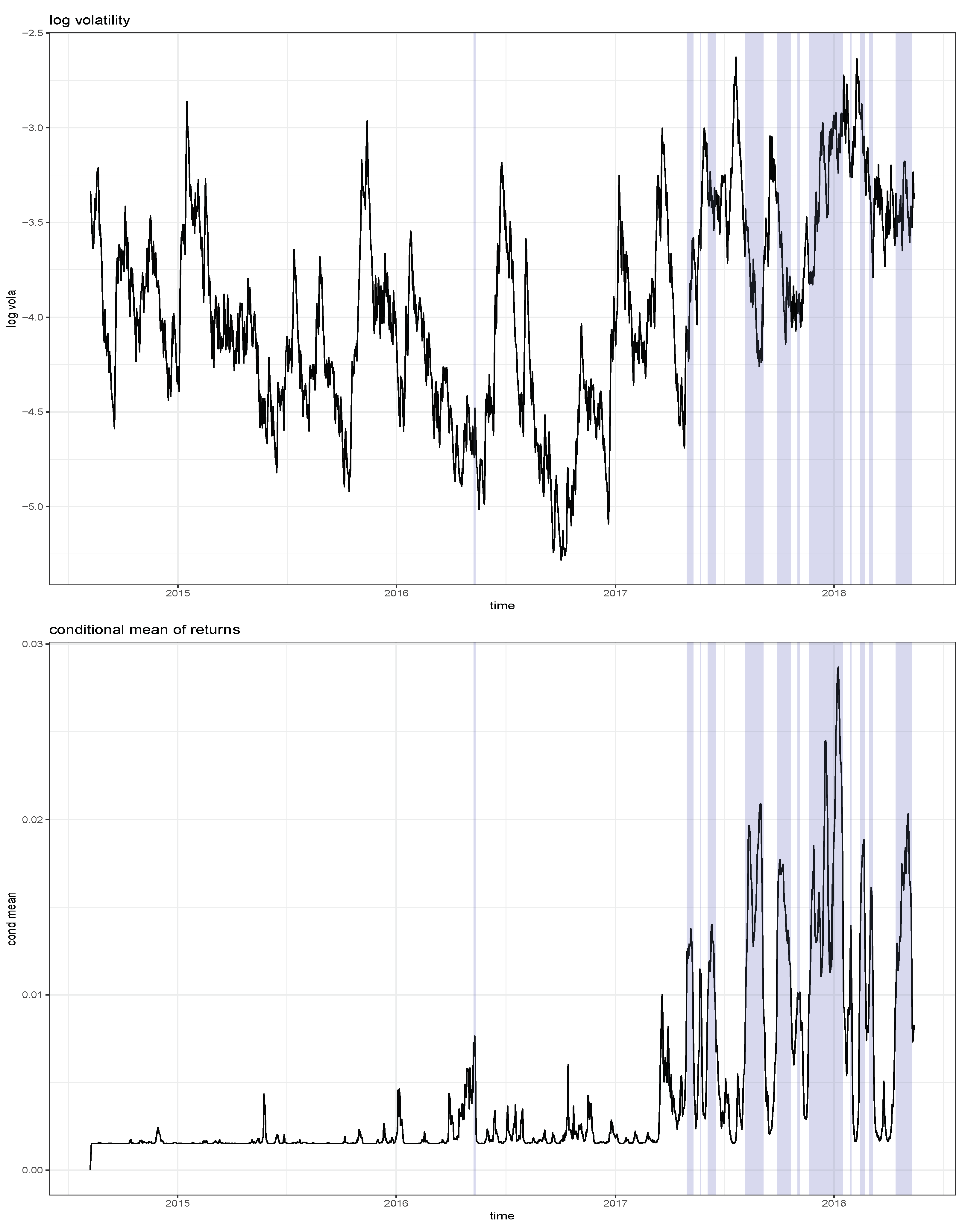
Figure 4 shows the estimated log volatility process together with the estimated conditional mean of returns, i.e., . The shaded areas highlight the estimated bubble periods, which mainly occurred in 2017 and parts of 2018. Not surprisingly, the shaded bubble periods correspond to substantially higher conditional mean returns, while it is close to zero for the non-shaded areas. Unlike Hafner (2018) who finds a single bubble regime starting in May 2017 and whose sample ends in December 2017, we find multiple bubble periods, mainly during the period May 2017 to April 2018. Hence, the starting date of these periods coincides with the single regime of Hafner (2018), but, due to the volatility of the sentiment index, this regime is decomposed into several sub-regimes. While the procedure advocated by (Hafner 2018; Phillips et al. 2011) identifies bubble periods that are of long duration and quite inert to price decreases, our approach produces regimes of shorter duration because, as the sentiment index drops, one quickly leaves a bubble regime.
Furthermore, we find that volatility is generally higher in the bubble regimes, with an average log volatility of −3.58 compared with −4.04 outside of a bubble. However, short term movements of volatility tend to react negatively to changes of the sentiment index, as reflected by the negative estimate of in model (2). Hence, our approach of using a sentiment index for modelling cryptocurrencies not only identifies locally explosive bubble periods, but also measures its impact on volatility. Moreover, it can be used as a predictive device, on a daily basis, both for returns and volatility. The method we propose conveys regulation implications in the cryptocurrency markets. Very likely scams come to a play given investors’ irrational exuberance and a surge of initial coin offerings (ICOs). However, these challenge the regulators in the presence of bubbles.
4. Conclusions
Our model allows to test for speculative bubbles in cryptocurrencies using a sentiment index, which drives the transition in a regime switching autoregression. For a popular cryptocurrency index, we find statistically significant regime nonlinearity and identify corresponding bubble periods. Furthermore, volatility is specified as a score-driven EGARCH-type model augmented with the daily changes of the sentiment index. We find that volatility increases as the sentiment index decreases, and vice versa. This is similar to the leverage effect in classical financial markets, where bad news have a stronger effect on volatility than good news, but here this effect is explicitly driven by the sentiment index.
Several extensions of the present analysis are possible. First, it is possible to do forecasting. One-step-ahead forecasting is trivial, but multi-step ahead is not, due to the nonlinearity of the conditional mean function. Several approaches could be employed including bootstrap and Monte Carlo simulation—see, e.g., van Dijk et al. (2002). In addition, the time series properties of the sentiment index would have to be investigated to build a model that explicitly takes the sentiment dynamics into account. Second, we could compare the statistical properties of our testing approach with those of a pure time series based approach such as Phillips et al. (2011). The latter approach uses less information and hence should have less power if the true data generating process is close to a smooth transition autoregression. This is left for future research.
Author Contributions
Both authors contributed equally to all parts of the manuscript.
Funding
This research was funded by grant ARC 18/23-089 of the Belgian government and the Deutsche Forschungsgemeinschaft through IRTG 1792 “High Dimensional Non Stationary Time Series”.
Conflicts of Interest
The authors declare no conflict of interest.
References
- Avery, Christopher N., Judith A. Chevalier, and Richard J. Zeckhauser. 2016. The “caps” prediction system and stock market returns. Review of Finance 20: 1363–81. [Google Scholar] [CrossRef]
- Bauwens, Luc, Christian M Hafner, and Sébastien Laurent. 2012. Volatility models. In Handbook of Volatility Models and Their Applications. Edited by Luc Bauwens, Christian M. Hafner and Sébastien Laurent. New York: John Wiley& Sons, chp. 1. pp. 1–50. [Google Scholar]
- Black, Fischer. 1976. Studies in stock price volatility changes. In Proceedings of the American Statistical Association, Business and Economic Statistics Section. Washington, DC: American Statistical Association, pp. 177–81. [Google Scholar]
- Cheah, Eng-Tuck, and John Fry. 2015. Speculative bubbles in bitcoin markets? An empirical investigation into the fundamental value of bitcoin. Economics Letters 130: 32–36. [Google Scholar] [CrossRef]
- Chen, Cathy Y. H., Romeo Després, Li Guo, and Thomas Renault. 2018. What Makes Cryptocurrencies Special? Investor Sentiment and Price Predictability in the Absence of Fundamental Value, Discussion Paper Sfb 649. Unpublished work.
- Cheung, Adrian, Eduardo Roca, and Jen-Je Su. 2015. Crypto-currency bubbles: An application of the Phillips-Shi-Yu (2013) methodology on Mt.Gox bitcoin prices. Applied Economics 47: 2348–58. [Google Scholar] [CrossRef]
- Christie, Andrew A. 1982. The stochastic behavior of common stock variances: Value, leverage and interest rate effects. Journal of Financial Economics 10: 407–32. [Google Scholar] [CrossRef]
- Conrad, Christian, Anessa Custovic, and Eric Ghysels. 2018. Long- and short-term cryptocurrency volatility components: A GARCH-MIDAS analysis. Journal of Risk and Financial Management 11: 23. [Google Scholar] [CrossRef]
- Corbet, Shaen, Brian Lucey, and Larisa Yarovaya. 2018. Datestamping the bitcoin and ethereum bubbles. Finance Research Letters 26: 81–88. [Google Scholar] [CrossRef]
- Creal, Drew, Siem Jan Koopman, and André Lucas. 2011. A dynamic multivariate heavy-tailed model for time-varying volatilities and correlations. Journal of Business & Economic Statistics 29: 552–63. [Google Scholar]
- De Long, J. Bradford, Andrei Shleifer, Lawrence H. Summers, and Robert J. Waldmann. 1990. Positive feedback investment strategies and destabilizing rational speculation. The Journal of Finance 45: 379–95. [Google Scholar] [CrossRef]
- Fry, John, and Eng-Tuck Cheah. 2016. Negative bubbles and shocks in cryptocurrency markets. International Review of Financial Analysis 47: 343–52. [Google Scholar] [CrossRef]
- Glosten, Lawrence R., and Paul R. Milgrom. 1985. Bid, ask and transaction prices in a specialist market with heterogeneously informed traders. Journal of Financial Economics 14: 71–100. [Google Scholar] [CrossRef]
- Granger, Clive W. J., and Timo Teräsvirta. 1993. Modelling Nonlinear Economic Relationships. Oxford: Oxford University Press. [Google Scholar]
- Gürkaynak, Refet S. 2008. Econometric tests of asset price bubbles: Taking stock. Journal of Economic Survey 22: 166–86. [Google Scholar] [CrossRef]
- Hafner, Christian. 2018. Testing for bubbles in cryptocurrencies with time-varying volatility. Journal of Financial Econometrics. [Google Scholar] [CrossRef]
- Harvey, Andrew C. 2013. Dynamic Models for Volatility and Heavy Tails. Cambridge: Cambridge University Press. [Google Scholar]
- Kim, Soon-Ho, and Dongcheol Kim. 2014. Investor sentiment from internet message postings and the predictability of stock returns. Journal of Economic Behavior & Organization 107: 708–29. [Google Scholar]
- Kjaerland, Frode, Aras Khazal, Erlend A. Krogstad, Frans B. G. Nordstroem, and Are Oust. 2018. An analysis of bitcoin’s price dynamics. Journal of Risk and Financial Management 11: 63. [Google Scholar] [CrossRef]
- Kruse, Robinson, and Christoph Wegener. 2019. Time-varying persistence in real oil prices and its determinant. Energy Economics. [Google Scholar] [CrossRef]
- Luukkonen, Saikkonen, and Teräsvirta. 1988. Testing linearity against smooth transition autoregressive models. Biometrika 75: 491–99. [Google Scholar] [CrossRef]
- Nasekin, Sergey, and Cathy Yi-Hsuan Chen. 2018. Deep Learning-Based Cryptocurrency Sentiment Construction. Available at SSRN 3310784. Available online: https://papers.ssrn.com/sol3/papers.cfm?abstract_id=3310784 (accessed on 29 March 2019).
- Nelson, Daniel B. 1991. Conditional heteroskedasticity in asset returns: A new approach. Econometrica 59: 347–70. [Google Scholar] [CrossRef]
- Pavlidis, Efthymios G., Ivan Paya, and David A. Peel. 2017. Testing for speculative bubbles using spot and forward prices. International Economic Review 58: 1191–226. [Google Scholar] [CrossRef]
- Pavlidis, Efthymios G., Ivan Paya, and David A. Peel. 2018. Using market expectations to test for speculative bubbles in the crude oil market. Journal of Money, Credit and Banking 50: 833–56. [Google Scholar] [CrossRef]
- Pesaran, M. Hashem, and Ida Johnsson. 2018. Double-question survey measures for the analysis of financial bubbles and crashes. Journal of Business & Economic Statistics, 1–15. [Google Scholar] [CrossRef]
- Phillips, Peter C. B., Shuping Shi, and Jun Yu. 2015. Testing for multiple bubbles: Historical episodes of exuberance and collapse in the s&p 500. International Economic Review 56: 1043–78. [Google Scholar]
- Phillips, Peter C. B., Yangru Wu, and Jun Yu. 2011. Explosive behavior in the 1990s nasdaq: When did exuberance escalate asset values? International Economic Review 52: 201–26. [Google Scholar] [CrossRef]
- Teräsvirta, Timo. 1994. Specification, estimation, and evaluation of smooth transition autoregressive models. Journal of the American Statistical Association 89: 208–18. [Google Scholar]
- Trimborn, Simon, and Wolfgang Karl Härdle. 2018. Crix an index for cryptocurrencies. Journal of Empirical Finance 49: 107–22. [Google Scholar] [CrossRef]
- van Dijk, Dick, Timo Teräsvirta, and Philip Hans Franses. 2002. Smooth transition autoregressive models—A survey of recent developments. Econometric Reviews 21: 1–47. [Google Scholar] [CrossRef]
- Yang, Fuyu, and Alasdair Brown. 2016. The Role of Speculative Trade in Market Efficiency: Evidence from a Betting Exchange. Review of Finance 21: 583–603. [Google Scholar]
| 1 | |
| 2 | This list can be found at https://api.stocktwits.com/symbol-sync/symbols.csv. |
Figure 1.
Structure of an LSTM unit.

Figure 2.
Log CRIX (upper panel) and sentiment index (lower panel). The shaded areas correspond to the estimated bubble periods.
Figure 2.
Log CRIX (upper panel) and sentiment index (lower panel). The shaded areas correspond to the estimated bubble periods.

Figure 3.
Estimated transition function. The vertical red line indicates the line , for which . Values above this line, i.e., the shaded area, are interpreted as the bubble regime.
Figure 3.
Estimated transition function. The vertical red line indicates the line , for which . Values above this line, i.e., the shaded area, are interpreted as the bubble regime.

Figure 4.
Estimated log volatility (upper panel) and conditional mean (lower panel). The shaded areas correspond to the estimated bubble periods.
Figure 4.
Estimated log volatility (upper panel) and conditional mean (lower panel). The shaded areas correspond to the estimated bubble periods.


Table 1.
Estimation results for the model without (M0) and with (M1) sentiment index. Standard errors are in parentheses. is the value of the log likelihood function.
Table 1.
Estimation results for the model without (M0) and with (M1) sentiment index. Standard errors are in parentheses. is the value of the log likelihood function.
| Parameter | Model M0 | Model M1 | ||
|---|---|---|---|---|
| −0.0929 | (0.0323) | −0.0972 | (0.0085) | |
| 0.1193 | (0.0155) | 0.1183 | (0.0153) | |
| 0.9759 | (0.0081) | 0.9709 | (0.0000) | |
| 0.3716 | (0.0325) | 0.3872 | (0.0330) | |
| 0.0025 | (0.0005) | 0.0015 | (0.0006) | |
| −0.0222 | (0.0392) | |||
| 0.7461 | (0.1461) | |||
| 0.0061 | (0.0012) | |||
| −0.2740 | (0.1289) | |||
| 2820.45 | 2838.78 | |||
© 2019 by the authors. Licensee MDPI, Basel, Switzerland. This article is an open access article distributed under the terms and conditions of the Creative Commons Attribution (CC BY) license (http://creativecommons.org/licenses/by/4.0/).
Share and Cite
MDPI and ACS Style
Chen, C.Y.-H.; Hafner, C.M. Sentiment-Induced Bubbles in the Cryptocurrency Market. J. Risk Financial Manag. 2019, 12, 53. https://doi.org/10.3390/jrfm12020053
AMA Style
Chen CY-H, Hafner CM. Sentiment-Induced Bubbles in the Cryptocurrency Market. Journal of Risk and Financial Management. 2019; 12(2):53. https://doi.org/10.3390/jrfm12020053
Chicago/Turabian StyleChen, Cathy Yi-Hsuan, and Christian M. Hafner. 2019. "Sentiment-Induced Bubbles in the Cryptocurrency Market" Journal of Risk and Financial Management 12, no. 2: 53. https://doi.org/10.3390/jrfm12020053